Reionization by Hard Photons: I.
X-rays from the First Star Clusters

Abstract

Observations of the Ly$\alpha$ forest at $z\sim 3$ reveal an average metallicity ${\rm Z}\sim 10^{-2}Z_{\odot}$. The high-redshift supernovae that polluted the IGM also accelerated relativistic electrons. Since the energy density of the CMB $\propto(1+z)^{4}$, at high redshift these electrons cool via inverse Compton scattering. Thus, the first star clusters emit X-rays. Unlike stellar UV ionizing photons, these X-rays can escape easily from their host galaxies. This has a number of important physical consequences: (i) Due to their large mean free path, these X-rays can quickly establish a universal ionizing background and partially reionize the universe in a gradual, homogeneous fashion. If X-rays formed the dominant ionizing background, the universe would have more closely resembled a single-phase medium, rather than a two-phase medium. (ii) X-rays can reheat the universe to higher temperatures than possible with UV radiation. (iii) X-rays counter the tendency of UV radiation to photo-dissociate ${\rm H_{2}}$, an important coolant in the early universe, by promoting gas phase ${\rm H_{2}}$ formation. The X-ray production efficiency is calibrated to local observations of starburst galaxies, which imply that $\sim 10\%$ of the supernova energy is converted to X-rays. While direct detection of sources in X-ray emission is difficult, the presence of relativistic electrons at high redshift and thus a minimal level of X-ray emission may be inferred by synchrotron emission observations with the Square Kilometer Array. These sources may constitute a significant fraction of the unresolved hard X-ray background, and can account for both the shape and amplitude of the gamma-ray background. This paper discusses the existence and observability of high-redshift X-ray sources, while a companion paper models the detailed reionization physics and chemistry.

1 Introduction

While the theoretical literature on the epoch of reionization is large and increasing rapidly, our empirical knowledge of this period in the history of the universe is scant and may be succintly summarized: (i) The universe is likely to have been reionized in the period $5.8<z_{r}<35$, where the lower bound arises from the lack of Gunn-Peterson absorption in the spectra of high redshift quasars (Fan et al 2000), and the upper bound comes from the observation of small scale power in Cosmic Microwave Background anistropies (Griffiths et al 1999). In CDM cosmologies, non-linear objects above the cosmological Jeans mass $10^{4-5}M_{\odot}$ first collapse during this period. (ii) The presence of metals in the Ly$\alpha$ forest implies that significant star formation took place at high redshift (Songailia & Cowie 1996, Songailia 1997). (iii) COBE constraints on the Compton y-distortion of the CMB (Wright et al, 1994, Fixsen et al 1996) implies that the IGM was not heated to high temperatures. This means it is unlikely that the hydrogen and helium in the IGM were collisionally reionized.

Thus, the current state of observations is consistent with scenarios in which the universe was reionized by an early generation of stars or quasars. While we do not know whether stars or quasars were the dominant source of ionizing photons, the observational and theoretical case for quasars is somewhat more uncertain. Extrapolation of empirical quasar luminosity functions to high redshift do not yield enough ionizing photons to maintain the observed lack of Gunn-Peterson absorption at $z\sim 5$ (Madau, Haardt & Rees 1999). The requisite steepening of the faint end slope at high redshift necessary to boost ionizing photon production is constrained by the lack of red, point-like sources in the Hubble Deep Field (Haiman, Madau & Loeb 1999); the authors find that AGN formation must have been suppressed in halos with $v_{c}<50-75\,{\rm km\,s^{-1}}$. We do not have a sufficiently firm understanding of the formation and fueling of supermassive black holes to assert on theoretical grounds that AGNs must have been present at high redshift. On the other hand, a minimal level of high-redshift star formation is guaranteed by the observed metal pollution of the IGM.

Theoretical scenarios in which stars or quasars figure predominantly have been calculated in detail. Our ignorance of the efficiency of gas fragmentation, and star/black hole formation as a function of halo mass, make the prediction of observable differences between these two scenarios very uncertain. Indeed, if one normalizes assumed emissivities to a fixed reionization epoch, differences between the two scenarios boil down to: (i) stars result in supernovae, which inject dust, metals, and entropy into the host galaxy and surrounding IGM, which affects subsequent chemistry and cooling, (ii) quasars have a significantly harder spectrum than stars. In particular, they produce X-rays.

In this paper, I emphasize a hitherto neglected fact: high redshift supernova also produce X-rays, both by thermal emission from the hot supernova remnant, and inverse Compton scattering of soft photons by relativistic electrons accelerated by the supernova. Considerable X-ray emission is already observed in starburst galaxies at low redshift (e.g., Rephaeli et al 1995), and the efficiency of most proposed X-ray production mechanisms should increase with redshift (e.g., explosions take place in a denser medium at high redshift, hardening expected thermal emission; inverse Compton scattering becomes more efficient since the CMB provides a ready supply of soft photons $U_{CMB}\propto(1+z)^{4}$). Thus, the SED of high-redshift star forming regions is considerably harder than has been previously assumed. This blurs the distinction between stellar/quasar reionization scenarios, and has a number of important physical consequences:

• Escape fraction The escape fraction of UV ionizing photons in the local universe is small, $\sim 3-6\%$ (Leitherer et al 1995, Bland-Hawthorne & Maloney 1999, Dove, Shull & Ferrara 2000) and is expected to decrease with redshift (Wood & Loeb 1999, Ricotti & Shull 1999). On the other hand, X-rays can escape freely from the host galaxy. Thus, processing by the host ISM may imply that the universe was reionized by a significantly harder spectrum than previously assumed.

• Reionization topology Photons from stellar spectra have a short mean free path and thus a sharply defined ionization front. This fact gives rise to the conventional picture of expanding HII bubbles embedded in the neutral IGM. The spectra of quasars is significantly harder and exert an influence over a larger distance (which is why it is much more difficult to perform numerical simulations of reionization by quasars; see Gnedin 1999). Nonetheless, for quasars, $\nu L_{\nu}\propto\nu^{-0.8}$ (Zheng et al 1997, although note that the observations were only in the radio-quiet AGN subsample at energies up to 2.6 Ry) and most of the energy for ionization lies just above the Lyman edge. Thus, there is still a sharply defined HII region and a thin ionization front where the ionization fraction drops sharply. By contrast, for the inverse Compton case $\nu L_{\nu}\sim{\rm const}$, there is equal power per logarithmic interval, and thus there is no preferred energy scale. In particular, there is no preferred scale for the mean free path of ionizing photons. When the universe is largely neutral, it is optically thick even to hard photons and all photons with energies $E<E_{thick}=1.5\left(\frac{1+z}{10}\right)^{0.5}x_{HI}^{1/3}\,{\rm keV}$ (where $x_{HI}$ is the mean neutral fraction) are absorbed across a Hubble volume. While the (more numerous) soft photons can only travel a short distance before ionizing neutral HI and HeI, the (less numerous but more energetic) hard photons will be able to travel further and ionize an equivalent number of photons by secondary ionizations. Thus, even if sources are distributed very inhomogeneously, reionization will be a fairly homogeneous event, with a largely uniform ionizing background and fluctuations in ionization fraction determined mainly by gas clumping. Instead of an two-phase medium in whose HII filling fraction increases with time, the early IGM may have been a single phase medium whose ionization fraction increases with time.

• Increased reheating A hard spectrum can reheat the IGM to considerably higher temperatures than soft stellar spectra, both through photoionization heating and Compton heating. A soft spectrum loses thermal contact with the IGM once HI and HeI are completely ionized (at the mean IGM density, HI has a recombination time longer than the Hubble time for $z<10$), and the gas cools adiabatically due to the expansion of the universe (Hui & Gnedin 1997). By contrast, a hard spectrum can continually transfer large amounts of energy from the radiation field to the IGM by ionizing HeII, which recombines rapidly (Miralda-Escude & Rees 1994). This feedback mechanism is important in increasing the Jeans mass, a proposed mechanism for preventing excessive cooling and star formation at high redshift (e.g., Prunet & Blanchard 1999). The higher IGM temperatures may also explain why observed Ly$\alpha$ forest line widths are commonly in excess of that predicted by numerical simulations (Theuns et al 1999, Ricotti et al 2000).

• Early universe chemistry ${\rm H_{2}}$ is an extremely important coolant in the metal-free early universe. While the neutral IGM is optically thick to UV ionizing photons, it is optically thin to photons longward of the Lyman limit (except at wavelengths corresponding to higher order hydrogen Lyman resonance lines, as well as $H_{2}$ resonance lines). In particular, photons in the 11.2-13.6 eV range quickly establish a soft UV background which photodissociates ${\rm H}_{2}$ via the Solomon process, shutting down subsequent star formation (Haiman, Rees & Loeb 1997, Cicardi, Ferrara & Abel 1998), unless the $H_{2}$ opacity is sufficient to reduce the photo-dissociation rate (Ricotti, Gnedin & Shull 2000). If X-rays are present in the early universe, they can counter this $H_{2}$ destruction. The IGM is also optically thin to X-rays, which can penetrate dense clouds of gas and promote gas phase ${\rm H_{2}}$ formation ${\rm H+e^{-}\rightarrow H^{-}+\gamma}$ and ${\rm H^{-}+H\rightarrow H_{2}+e^{-}}$ by increasing the abundance of free electrons. Haiman, Abel & Rees (1999) show that if quasars were the dominant ionizing sources in the early universe, gas cooling and thus star formation can continue unabated. In Paper II, I show that in fact even if only stars were present, a self-consistent treatment of the stellar SED incorporating X-rays produced by supernovae favours ${\rm H_{2}}$ formation over destruction in dense regions.

In this paper, I study the emission mechanisms and observational signatures of X-ray bright star clusters at high redshift. In Paper II (Oh 2000a), I address the changes in reionization topology, reheating and early universe chemistry mentioned above due to these X-rays.

In all numerical estimates, I assume a background cosmology given by the ’concordance’ values of Ostriker & Steinhardt (1995): $(\Omega_{m},\Omega_{\Lambda},\Omega_{b},h,\sigma_{8h^{-1}},n)=(0.35,0.65,0.04,0.65,0.87,0.96)$. This corresponds to $\Omega_{b}h^{2}=0.017$, compared with $\Omega_{b}h^{2}=0.020\pm 0.002\,(95\%{\rm c.l.})$ (Burles, Nollett & Turner 2000), and $\Omega_{b}h^{2}=0.0205\pm 0.0018$ (O’Meara et al 2000) from Big Bang Nucleosynthesis, and the significantly higher values $0.022<\Omega_{b}h^{2}<0.040(95\%{\rm c.l.})$ (Tegmark & Zaldarriaga 2000) preferred by recent CMB anisotropy data, such as Boomerang and Maxima.

2 Emission mechanisms

2.1 Star formation at $z>3$

What fraction of present day stars formed at high redshift? Estimates of the comoving star formation rate as a function of redshift (Madau et al, 1996) should be regarded as lower bounds, particularly at high redshift, due to the unknown effects of dust extinction, and star formation in faint systems below the survey detection threshold. Indeed, Lyman break survey results for $3.6<z<4.5$ (Steidel et al 1999) suggest that after correction for dust extinction, the comoving star formation rate for $z>1$ is constant, rather than falling sharply as previously believed. Furthermore, in recent years compelling evidence has emerged that the majority of stars in ellipticals and bulges formed at high redshift, $z>3$. This comes from the tightness of correlations between various global properties of ellipticals which indicate a very small age dispersion and thus a high redshift of formation, unless their formation was synchronized to an implausible degree. The evidence includes the tightness of the fundamental plane and color magnitude relations for ellipticals, and the modest shift in zero-points for these relations with redshift (Renzini 1998 and references therein). Since spheroids contain $\sim 30\%$ of all stars in the local universe (King & Ellis 1985, Schechter & Dressler 1987), this would imply that $\sim 30\%$ of all stars have formed at $z>3$. Since $\sim 20\%$ of baryons have been processed into stars by the present day (Fukugita, Hogan & Peebles 1998), this implies that $\sim 0.2\times 0.3\sim 6\%$ of baryons have been processed into stars by $z\sim 3$. Assuming widespread and uniform enrichment and 1 ${\rm M_{\odot}}$ of metals per 100 ${\rm M_{\odot}}$ of stars formed, this translates into an IGM metallicity of $6\times 10^{-4}\sim 3\times 10^{-2}Z_{\odot}$. At $z\sim 3$, the metallicity of damped Ly$\alpha$ systems appears to be $\sim 0.05Z_{\odot}$ (Pettini et al 1997), in reasonable agreement. The observed metallicity of the Ly$\alpha$ forest at $z\sim 3$, to which most models of reionization have been normalized, is between $10^{-2}Z_{\odot}$ and $10^{-3}Z_{\odot}$ (Songailia & Cowie 1996, Songailia 1997), which would imply that only $0.2-2\%$ of present day stars formed at $z>3$. However, its metallicity may be more representative of low density regions, rather than the mean cosmological metallicity (Cen & Ostriker 1999). Note that normalization of high redshift star formation to Lyman $\alpha$ forest metallicities assume efficient metal ejection (which underestimates star formation if a significant fraction of metals are retained) and mixing (which overestimates star formation if Ly$\alpha$ lines are preferentially observed in overdense regions which are sites of star formation). In this context, it is worth mentioning claims that Ly$\alpha$ lines with $10^{13.5}{\rm cm^{-2}}<{\rm N_{HI}}<10^{14.5}\,{\rm cm^{-2}}$ reveal lower metallicities by a factor of 10 than clouds with ${\rm N_{HI}}>10^{14.5}\,{\rm cm^{-2}}$ (Lu et al 1999). Ellison et al (2000) find no break in the power law column density distribution for C IV down to log N(C IV) =11.7, and Schaye et al (2000) detect O VI down to $\tau_{HI}\sim 10^{-1}$ in underdense gas, so it appears that metal pollution was fairly widespread. I regard ${\rm Z}\sim 10^{-3}-2.5\times 10^{-2}Z_{\odot}$ at $z\sim 3$ as a fairly firm bracket on the range of possibilities. For inverse Compton radiation, this corresponds to an energy release per IGM baryon of $\epsilon^{SN}\sim 10\left(\frac{Z}{10^{-2}Z_{\odot}}\right)\left(\frac{\epsilon}{0.1}\right)$eV (where $\epsilon$ is the efficiency of conversion of supernova energy to X-rays), which is comparable to the energy release in stellar UV radiation for the low escape fractions expected, $\epsilon^{stellar}\sim 10\left(\frac{Z}{10^{-2}Z_{\odot}}\right)\left(\frac{f_{esc}}{0.01}\right)$eV, where $f_{esc}$ is the escape fraction of ionizing photons from the source.

2.2 X-ray emission in local starbursts

Most models of reionization use population synthesis codes to estimate the spectral energy distribution of starbursts. However, there are many processes associated with star formation that generate UV and X-rays, beside stellar radiation: massive X-ray binaries, thermal emission from supernova remnants and hot gas in galactic halos and winds, inverse Compton scattering of soft photons by relativistic electrons produced in supernovae. Indeed, X-ray emission appears to be ubiquitous among starbursts (e.g., Rephaeli, Gruber, & Persic 1995), and starburst galaxies may account for a significant portion of the XRB (Bookbinder et al 1980, Rephaeli et al 1991, Moran, Lehnert & Helfand 1999). The X-ray emission from these processes, which hardens the spectrum of starbursts and changes both the topology and chemistry of reionization, has to date been neglected in studies of the $z>5$ universe.

The X-ray luminosity of starbursts correlates well with other star formation indicators; for example, David et al (1992) find a roughly linear relation between $L_{FIR}$ and $L_{X}$. As a very rough empirical calibration, the starburst galaxies M82 & NGC 3256 observed with ROSAT and ASCA (Moran & Lehnert 1997, Moran, Lehnert & Helfand, 1999) follow the relations (after correction for absorption): $L_{X,0.2-10\,{\rm keV}}=8\times 10^{-4}L_{IR}$, and $L_{X,5\,{\rm keV}}=1.2\times 10^{4}L_{R,5\,{\rm GHz}}$ (note that 5 keV flux density is relatively unaffected by photoelectric absorption or soft thermal emission). The starburst model of Leitherer and Heckman (1995) yields $L_{bol}\sim L_{{\rm FIR}}\sim 1.5\times 10^{10}({\rm SFR}/1\,{\rm M_{\odot}yr^{-1}})L_{\odot}$; as a cross-check, the empirical relation for radio emission is (Condon 1992) $L_{R}=1.4\times 10^{28}(\nu/{\rm GHz})^{-\alpha}({\rm SFR}/{\rm M_{\odot}yr^{-1}})\,{\rm erg\,s^{-1}\,Hz^{-1}}$, where $\alpha\sim 0.8$. Together I obtain:

$$L_{X}=5\times 10^{40}\left(\frac{SFR}{1\,{\rm M_{\odot}yr^{-1}}}\right)\ \ {\rm erg\,s^{-1}}$$ (1)

One should not regard this as more than a rough order of magnitude estimate; a large scatter is expected in this relation. By way of comparison, Rephaeli et al (1995) obtain from the mean of 51 starbursts observed with Einstein and HEAO, $L_{X,2-30\,{\rm keV}}\sim 8\times 10^{-3}L_{IR}$, an order of magnitude greater; and David et al (1992) obtain from a sample of 71 normal and starburst galaxies a ratio lower by about an order of magnitude, largely due to the inclusion of normal galaxies (this is consistent with an inverse Compton origin for X-rays, since normal galaxies have much lower radiation field energy densities and would not be expected to show significant inverse Compton emission).

The typical observed X-ray spectrum is a power-law, $L_{\nu}\propto\nu^{-0.8}$, consistent with a non-thermal origin. An obscured AGN is not likely to be the source of these X-rays, as several observations suggest that the X-ray emission is powered primarily by massive stars. In NGC 3256, observations by ISO fail to detect high excitation emission lines (Rigopoulou et al 1996). In M82, the optical spectrum is HII-like (Kennicutt 1992), discrete nuclear radio sources are spatially resolved (Muxlow et al 1994), its nuclear X-ray emission is extended (Bregman et al 1995), and the expected broad H$\alpha$ emission is not detected (Moran & Lehnert 1997); the HEX continuum and Fe-K line emission of NGC 253 as observed by BeppoSAX is extended (Cappi et al 1999). Moran & Lehnart (1997) and Moran, Lehnart, & Helfand (1999) have modelled the X-ray emission of M82 and NGC 3256, and find inverse-Compton emission to be the most likely mechanism, rather than an obscured AGN or massive X-ray binaries. The ratio between the observed radio and X-ray fluxes (note that $L_{X}/L_{syn}\propto U_{IR}/U_{B}$, where $U_{IR}$ is the energy density of the infra-red radiation field, and $U_{B}$ is the energy density of the magnetic field) is consistent with an inverse-Compton origin for the X-rays. Furthermore, the X-ray and radio emission have the same spectral slope, as is expected if both types of emission are non-thermal, arising from the same population of electrons. The X-ray luminosity is energetically consistent with a star formation origin. Assuming a Salpeter IMF and that each supernova explosion yields $10^{51}$ erg in kinetic energy yields an energy injection rate into the ISM:

$$\dot{E}_{SN}\sim 3\times 10^{40}{\rm\left(\frac{SFR}{1M_{\odot}\,yr^{-1}}\right)}\left(\frac{\epsilon}{0.1}\right)\,{\rm erg\,s^{-1}}$$ (2)

where $\epsilon$ is the fraction of energy injected into relativistic electrons; consistency with the observed value, (1), implies that $\epsilon\sim 10\%$. Hereafter, I shall use the empirical equation (1) as a fiducial conversion between X-ray luminosity and star formation rate.

Is an acceleration efficiency of $\epsilon\sim 10\%$ reasonable? The acceleration mechanism for relativistic electrons is poorly understood. While first-order Fermi acceleration in shocks is widely accepted as the acceleration mechanism for cosmic rays (Blandford & Eichler 1987, Jones & Ellison 1991), the electron acceleration is thought to be more problematic, due to the smaller electron gyroradius (which leads to greater difficulties in bouncing an electron back and forth across a shock of finite thickness), and the difficulty of initially boosting the electron to relativistic speeds, where Fermi acceleration can operate (Levinson 1994). From measurements of cosmic rays energy density it is inferred that $\sim 10\%$ of the supernova kinetic energy, or $\sim 10^{50}$erg per explosion, is liberated as cosmic rays (Volk, Klein, & Wielebinski 1989), but the division between electrons and protons at the source is not known. Since the measured ratio of cosmic ray protons to electrons is $\sim 75$ (e.g., Gaisser 1990), it might well be that relativistic electrons only constitute $\epsilon\sim 10^{-3}$ of the supernova energy budget. Thus, the reader should be cautioned that $\epsilon\sim 0.1$, which corresponds roughly equal energy division between protons and electrons (e/p=1), may be an overly optimistic estimate of the energy injection into relativistic electrons. Theoretical models of shock acceleration, in which e/p is a free parameter, often set e/p$\sim 1-5\%$ for consistency with cosmic-ray experiments (Ellison & Reynolds 1991, Ellison et al 2000). However, this is somewhat model-dependent: in models where electrons are injected directly from the thermal pool, $\sim 5\%$ of the energy in the shock must go to non-thermal electrons in order to match gamma-ray observations (Bykov et al 2000). Furthermore, note that the observed cosmic-ray e/p ratio could equally well be the result of different transport processes and energy loss mechanisms for electrons and protons. In particular, cosmic ray electrons are subject to loss processes which operate on much longer timescales for cosmic ray protons (inverse Compton, synchrotron losses, etc); the cosmic ray flux at earth for electrons could arise from a much smaller effective volume than that for protons. At the source, the energy division between protons and electrons could range between 1 and 100. Perhaps the most reliable means of inferring the proton/electron energy division is by direct observations of supernova remnants. In modelling the observed production of gamma-rays in the supernova remnants IC 443 and $\gamma$ Cygni observed by the EGRET instrument on the Compton Gamma Ray Observatory, Gaisser, Protheroe & Stanev (1998) find that a proton to electron ratio of 3–5 gives the best fit to the observed spectra, implying $\epsilon\sim 0.02-0.03$. Similarly, in modelling the $\gamma$-ray flux from 2EG J1857+0118 associated with supernova remnant W44, de Jager & Mastichiadis (1997) find $\epsilon\sim 0.09$. They speculate that electron injection by the pulsar may be responsible for the increased electron energy content. Given the large uncertainties, henceforth I shall simply use the empirical relation (1).

Thus, barring non-standard IMFs, type II detonation energies or alternate sources of relativistic electrons, the empirical relation (1) implies an acceleration efficiency $\epsilon\sim 0.1$ which is plausible but certainly lies at the upper limit of theoretical expectations. Another possibility is that the X-ray emission cannot be wholly attributed to inverse Compton emission alone (this assumption rests on the arguments of Moran & Lehnart (1997) and Moran, Lehnart, & Helfand (1999) with regards to the slopes and relative intensities of the observed non-thermal radio and X-ray emission). The X-ray emission may instead be due to X-ray binaries, thermal emission from supernova remnants or starburst driven superwinds (e.g., see Natarajan & Almaini 2000). It should be noted that only soft X-rays are relevant for reionization, since the universe is optically thin to photons with energies $E>E_{thick}=1.5\left(\frac{1+z}{10}\right)^{0.5}x_{HI}^{1/3}\,{\rm keV}$ (where $x_{HI}$ is the mean neutral fraction of the IGM). Since equation (1) is calibrated with the soft bands observed by ROSAT, this implies that even if $\epsilon\ll 0.1$ and the observed X-rays are not predominantly due to inverse Compton emission, the importance of X-rays for reionization (in particular, for changing the topology, for increased reheating, and increased $H_{2}$ production) may still hold. However, observational predictions which focus specifically on the inverse Compton mechanism (e.g., the gamma-ray background (section (3.2)), and detecting synchrotron emission with the SKA (section (3.4)) will no longer be valid. Since the acceleration efficiency is the most uncertain parameter in this paper, wherever relevant I insert the scaling factor $\left(\frac{\epsilon}{0.1}\right)$ into numerical estimates.

How does the X-ray luminosity compare with stellar UV ionizing radiation? Assuming a Salpeter IMF with solar metallicity, the Bruzual & Charlot (1999) population synthesis code yields an energy output of $L_{ion}=3.2\times 10^{42}({\rm SFR/1{\rm M_{\odot}\,yr^{-1}})\,{\rm erg\,s^{-1}}}$ in ionizing photons, which translates into ${\rm\dot{N}_{ion}}=10^{53}({\rm SFR}/1{\rm M_{\odot}\,yr^{-1}})\,{\rm photons\,s^{-1}}$. However, note that most of these ionizing photons are absorbed locally with the ISM of the star cluster; the escape fraction of ionizing photons into the IGM is expected to be small. Leitherer et al (1995) have observed four starburst galaxies with the Hopkins Ultraviolet Telescope (HUT). Their analyis suggests an escape fraction of only $3\%$, based on a comparison between the observed Lyman continuum flux and theoretical spectral energy distributions. For our own Galaxy, Dove, Shull & Ferrara (2000) find an escape fraction for ionizing photons of $6\%$ and $3\%$ (for coeval and Gaussian star formation histories respectively) from OB associations in the Milky Way disk. Bland-Hawthorn & Maloney (1999) find an escape fraction of $6\%$ is necessary for consistency with the observed H$\alpha$ emission from the Magellanic stream and high velocity clouds. On the other hand, a recent composite spectrum of 29 Lyman break galaxies (LBGs) with redshifts $\langle z\rangle=3.40\pm 0.09$ shows significant detection of Lyman continuum flux (Steidel, Pettini & Adelberger 2000); for typical stellar synthesis models, the observed flux ratio L(1500)/L(900)=$4.6\pm 1.0$ implies little or no photoelectric absorption. The fraction of 900 ${\rm\AA}$ photons which escape, $f_{esc}\sim 15-20\%$, is modulated almost entirely by dust absorption. Nonetheless, the authors themselves stress this result should be treated as preliminary; the result could be due to a large number of uncertainties or selection effects, among them the fact that these galaxies were selected from the bluest quartile of LBGs. On the theoretical side, radiative transfer calculations by Woods & Loeb (1999) find that the escape fraction at $z\sim 10$ is $<1\%$ for stars; calculations by Ricotti & Shull (1999) find that the escape fraction decreases strongly with increasing redshift and halo mass; for a $10^{9}\,M_{\odot}$ halo at $z=9$, the escape fraction is $\sim 10^{-3}$ (note that in the Ricotti & Shull (1999) models, the escape fraction rises towards low masses, and can be considerable for the halos with $M<10^{7}M_{\odot}$. Since such halos have $T_{vir}<10^{4}$K, their contribution to reionization depends on whether $H_{2}$ formation and cooling can take place despite photodissociative processes (Haiman, Rees & Loeb 1997, Cicardi, Ferrara & Abel 1998, Ricotti, Gnedin & Shull 2000)). For low escape fractions, the energy release in UV photons is roughly comparable to that in inverse-Compton X-rays :

$$L_{UV}=3\times 10^{40}\left(\frac{f_{esc}}{0.01}\right)\left(\frac{\rm SFR}{1{\rm M_{\odot}yr^{-1}}}\right)\,{\rm erg\,s^{-1}}$$ (3)

Note that to first order the ratio of stellar UV to inverse Compton X-rays is not sensitive to uncertainties in the IMF, as the same massive stars with $M>20M_{\odot}$ that dominate the Lyman continuum of a stellar population also explode as supernovae (however, see section (2.4) for some caveats).

Will X-ray emission still be efficient at high redshift? The following changes are expected to take place at high redshift: (i) The ISM is initially free of dust and metals, although rapid enrichment could occur on fairly short timescales ($t\sim 10^{6}-10^{7}$yr). (ii) The average ISM density is significantly higher, $n_{halo}\sim n_{0}18\pi^{2}(1+z)^{3}=0.02(\frac{1+z}{10})^{3}{\rm cm^{-3}}$ in a halo and $n_{disc}\sim\lambda^{-3}n_{halo}\sim 160(\frac{1+z}{10})^{3}{\rm cm^{-3}}(\lambda/0.05)^{-3}$ in a disk (where $\lambda$ is the spin parameter). A supernova remnant at high $z$ expands into a denser ISM: since it spends a shorter time in the Taylor-Sedov phase, most of its energy is radiated at a smaller radius, where the effective temperature is higher. This implies a harder spectrum for thermal emission. In addition, the density and temperature of gas in star forming regions is determined by the properties of ${\rm H}_{2}$ cooling (which saturates at $n\sim 10^{4}\,{\rm cm^{-3}}$ and $T\sim 300$K), rather than metal cooling as in the local universe. (iii) Potential wells are significantly shallower, so pressurised regions (hot gas, strong magnetic fields) cannot be efficiently confined. (iv) The CMB energy density $U_{CMB}\propto(1+z)^{4}$, so inverse Compton radiation becomes particularly efficient at high redshift. Because of (iii) and (iv), relativistic electrons cool predominantly by inverse Compton scattering rather than synchrotron emission. Since inverse Compton emission is likely to be the most promising mechanism for X-ray emission, I shall consider it at length.

2.3 Inverse Compton emission

The energy loss rate for a relativistic electron with Lorentz factor $\gamma$ is given by:

$$\dot{{\rm E}_{IC}}=\frac{4}{3}\sigma_{T}c\gamma^{2}U_{rad}=1.12\times 10^{-16}\left(\frac{1+z}{10}\right)^{4}\left(\frac{\gamma}{10^{3}}\right)^{2}\ {\rm erg\,s^{-1}}$$ (4)

for $U_{rad}=U_{\rm CMB}$. The loss rate by synchrotron radiation is given by substiting $U_{B}$ for $U_{rad}$, $\dot{{\rm E}_{synch}}=\frac{4}{3}\sigma_{T}c\gamma^{2}U_{B}$. In the local universe, galaxies with relatively quiescent star formation emit most of their electron energy in synchrotron radiation. Starbursts in the local universe can radiate efficiently in IC, as the energy density in the local radiation field is sufficiently high (typically, $U_{r}\sim 10^{-8}\,{\rm erg\,cm^{-3}}$ as opposed to $U_{r}\sim 10^{-12}\,{\rm erg\,cm^{-3}}$ in our Galaxy). Seed photons are provided by IR emission from dust grains. By contrast, at high redshift, all star forming regions will emit in inverse Compton radiation, as the CMB provides a universal soft photon bath of high energy density, $U_{CMB}=4\times 10^{-9}(\frac{1+z}{10})^{4}\,{\rm erg\,cm^{-3}}$. An electron with Lorentz factor $\gamma$ will boost a CMB photon of frequency $\nu_{o}$ to a frequency $\nu=\gamma^{2}\nu_{o}$. Thus, the rest frame frequency of a CMB photon (at the peak of the blackbody spectrum) which undergoes inverse Compton scattering is:

$${\rm E}_{IC}=600\left(\frac{\gamma}{300}\right)^{2}\left(\frac{1+z}{10}\right)\,{\rm eV}$$ (5)

Note that the observed frequency is independent of source redshift, since the higher initial frequency and redshifting effects cancel out.

Below, I examine in detail the mechanisms by which relativistic electrons lose energy, to see if indeed inverse Compton radiation will predominate.

2.3.1 Energy loss processes for relativistic electrons

Once relativistic electrons are produced, they can cool via a variety of mechanisms. Let us examine them in turn (for more details see Pacholczyk 1970, Daly 1992).

Synchrotron radiation The relative emission rate in inverse Compton and synchrotron emission is given simply by the relative energy densities in the radiation and magnetic fields, $\dot{E}_{IC}/\dot{E}_{syn}=U_{rad}/U_{m}$. This yields:

$$\frac{\dot{E}_{IC}}{\dot{E}_{syn}}=1.1\times 10^{3}\left(\frac{B}{10\mu G}\right)^{-2}\left(\frac{1+z}{10}\right)^{4}$$ (6)

Note that in energy loss terms the CMB may be characterized as having an effective magnetic field strength $B_{CMB,eff}=3.24\times 10^{2}\left(\frac{1+z}{10}\right)^{2}\ {\rm\mu G}$. Could magnetic fields in proto-galaxies possibly reach these high values? A reasonal assumption is that $P_{B}\sim P_{rel}<P_{gas}$, where $P_{B}$ is the magnetic field pressure, $P_{rel}$ is the pressure in relativistic particles, and $P_{gas}$ is the thermal gas pressure. Local observations of synchrotron and inverse Compton emission from radio galaxies are consistent with equipartition $P_{B}\sim P_{rel}$ (Kaneda et al 1995). I have assumed that the energy injection into relativistic particles is $\sim 10\%$ of the total kinetic energy of a supernova, so $P_{rel}<P_{gas}$ should be a strict upper bound. Thus, $P_{B}<P_{gas}$ gives the upper bound:

$$B<6\left(\frac{n}{1{\rm cm^{-3}}}\right)^{1/2}\left(\frac{T}{10^{4}K}\right)\,\mu G$$ (7)

where $n$ is the baryon number density (note that gas with temperatures $>10^{4-5}$K will escape from the shallow potential wells of the first proto-galaxies). If the magnetic field exceeds the above value, the over-pressurised lobe will expand on the dynamical time scale until the magnetic pressure drops. Thus, for $z>5$, it seems likely that synchrotron energy losses will be unimportant.

Ionization & Cherenkov losses Interactions with the non-relativistic gas will result in energy losses via ionization and Cherenkov emission of plasma waves at a rate independent of the Lorentz factor, $\dot{E}_{ion}\approx 9\times 10^{-19}n\,{\rm erg\,s^{-1}}$, which implies that the relative energy loss rate is:

$$\frac{\dot{E}_{IC}}{\dot{E}_{ion}}=120\left(\frac{n}{1{\rm cm^{-3}}}\right)^{-1}\left(\frac{1+z}{10}\right)^{4}\left(\frac{\gamma}{10^{3}}\right)^{2}$$ (8)

Thus, for

$$\gamma>\gamma_{break}\approx 100\left(\frac{n}{1{\rm cm}^{-3}}\right)^{1/2}(\frac{1+z}{10})^{-2}$$ (9)

inverse Compton losses are more important than ionization losses. The cutoff Lorenz factor at the lower end $\gamma_{co}$, is of interest since the lower end accounts for most of the electrons, both in terms of number and energy: $N_{electrons}(>\gamma)\propto\gamma^{-2\alpha}=\gamma_{co}^{-1.6}\$; $E_{electrons}(>\gamma)\propto\gamma^{-2\alpha+1}=\gamma_{co}^{-0.6}\ (\alpha=0.8)$. Note that the electrons that cool via ionization losses do not drop out completely, but merely form a flattened distribution with $\gamma_{f}\approx\gamma_{i}-350\,n({\rm t/10^{7}yr})$. These electrons with lower Lorentz factors could scatter CMB photons to optical and UV frequencies.

Free-free radiation Free-free radiation results in an energy loss rate $\dot{E}_{free-free}=6\times 10^{-22}n\gamma\,{\rm erg\,s^{-1}}$. Thus, free-free radiation only dominates over ionization and Cherenkov radation for $\gamma>1500$. However, in this regime inverse Compton losses dominate, since

$$\frac{\dot{E}_{IC}}{\dot{E}_{ff}}=190\left(\frac{n}{1cm^{-3}}\right)^{-1}\left(\frac{1+z}{10}\right)^{4}\left(\frac{\gamma}{10^{3}}\right)$$ (10)

Thus, free-free emission is never important in cooling relativistic electrons at high redshift.

In summary, the inverse Compton emission is the dominant energy loss mechanism between a lower and upper energy cutoff. From equation (9), the lower frequency break is determined by the competition between the inverse Compton loss rate and ionization and atomic cooling losses, below

$$E_{lower}=\gamma_{break}^{2}h\nu_{{\rm CMB}}=70\left({\rm\frac{{\rm n}}{1\,{\rm cm^{-3}}}}\right)\left(\frac{1+z}{10}\right)^{-3}\,{\rm eV},$$ (11)

where I assume the seed photon $\nu_{{\rm CMB}}=1.6\times 10^{12}\left(\frac{1+z}{10}\right)$GHz lies at the peak of the CMB blackbody spectrum. The competition between inverse Compton cooling losses and the rate of energy injection by Fermi acceleration determines the upper energy cutoff. The timescale for losses by inverse Compton radiation is:

$$t_{life}=\frac{E}{\dot{E}}=7.9\times 10^{5}\left(\frac{1+z}{10}\right)^{-4}\left(\frac{\bar{\gamma}}{300}\right)^{-1}\ {\rm years}$$ (12)

Equating the Fermi acceleration timescale $t_{acc}\sim r_{L}c/v_{sh}^{2}=1.3\times 10^{-3}\left(\frac{\gamma}{300}\right)\left(\frac{B}{10\mu G}\right)^{-1}\left(\frac{v_{sh}}{2000{\rm kms^{-1}}}\right)^{-2}$yr (where $r_{L}$ is the Larmour gyroradius, and $v_{sh}$ is the typical shock velocity) to $t_{life}$ (equation (12), I obtain for the maximum Lorentz factor $\gamma_{max}=7.4\times 10^{6}{\rm\left(\frac{B}{10\mu G}\right)}^{1/2}\left(\frac{v_{sh}}{2000\,{\rm km\,s^{-1}}}\right)\left(\frac{1+z}{10}\right)^{-2}$ which corresponds to an upper energy cutoff:

$$E_{upper}\sim 360{\rm\left(\frac{B}{10\mu G}\right)}\left(\frac{v_{sh}}{2000{\rm km\,s^{-1}}}\right)^{2}\left(\frac{1+z}{10}\right)^{-3}\,{\rm GeV}.$$ (13)

In section (2.3.2), I derive the form of the spectrum. For the power law spectrum obtained, $L_{\nu}\propto\nu^{-1}$, the specific luminosity depends only logarithmically on the energy cutoffs: $L_{\nu}=\frac{L_{tot}}{{\rm log(\nu_{upper}/\nu_{lower}})}\nu^{-1}$.

2.3.2 Inverse Compton spectrum

The Fermi shock acceleration mechanism for cosmic rays involves a steady growth of particle energy as a particle scatters back and forth across the shock front. This naturally produces a power law electron energy spectrum with energy spectrum $dn/d\gamma\propto\gamma^{-p}$, where $p=(\chi+2)/(\chi-1)$ and $\chi$ is the compression ratio for the shock (e.g., Jones & Ellison 1991). The final emission spectrum $L_{\nu}\propto\nu^{-\alpha}$ depends on the electron energy spectrum; the synchrotron or inverse Compton spectral index is $\alpha=(p-1)/2$. Thus, the spectral index is determined by the shock structure rather than the details of the scattering process. For a strong adiabatic shock $\chi=4$ and $dn/d\gamma\propto\gamma^{-2}$; for an isothermal shock, $\chi\gg 1$ and $dn/d\gamma\propto\gamma^{-1}$. The assumption of adiabaticity is most appropriate for the Taylor-Sedov phase, when most of the electrons are accelerated. Galactic SNR show a mean radio spectral index $\alpha=0.5\pm 0.15$ (Droge et al 1987), which agrees with $dn/d\gamma\propto\gamma^{-2}$. I shall use this as the canonical electron injection spectrum in this paper. The steepening of the diffuse synchrotron emission to $\alpha\sim 0.8$ is likely to be due to energy losses as the electrons age. I examine the emission spectrum in detail below. I assume that there is one supernova for every 100 $M_{\odot}$ of stars formed, that each supernova liberates $\sim 10^{51}$erg in kinetic energy, and $\sim 1M_{\odot}$ of metals.

The equation for the evolution of the electron population is given by (Ginzburg & Syrovatskii 1964, Sarazin 1999):

$$\frac{\partial N(\gamma)}{\partial t}=\frac{\partial}{\partial\gamma}[b(\gamma)N(\gamma)]+Q(\gamma)$$ (14)

where $N(\gamma)$ is the number of electrons in the range $\gamma$ to $\gamma+d\gamma$, the rate of production of new relavistic electrons is given by $Q(\gamma)$, and the rate of energy loss of an individual particle is given by $b(\gamma)\equiv d\gamma/dt$. From equation (12), we see that the electron lifetime is shorter than both the Hubble time for the redshifts under consideration $z<30$ and typical timescales for starbursts ($\sim 10^{7}$ years). We can thus assume that the electron population quickly reaches a steady state where the energy losses due to inverse Compton scattering (for high $\gamma$) and Coulomb collisions (for low $\gamma$) balance the injection rate due to supernova explosions, and set the time derivative to zero. Since injected electrons survive for less than a Hubble time, I ignore evolution in loss rate due to the evolution of the CMB energy density. Assuming that each supernova injects a population of electrons with $Q(\gamma)=Q_{o}\gamma^{-p}$, where $p\sim 2$, then the steady state solution to equation (14) is given by:

$$N(\gamma) = 4\times 10^{61}\left(\frac{1+z}{10}\right)^{-4}{\rm\left(\frac{SFR}{1M_{\odot}\,yr^{-1}}\right)}\gamma^{-(p+1)}\ \ \ ;\gamma>\gamma_{break}$$ (15)

$$N(\gamma) = 4\times 10^{57}\left({\rm\frac{{\rm n}}{1\,{\rm cm^{-3}}}}\right)^{-1}{\rm\left(\frac{SFR}{1M_{\odot}\,yr^{-1}}\right)}\gamma^{-(p-1)}\ \ \ ;\gamma<\gamma_{break}$$

where $\gamma_{break}$ (equation (9)) is the transition energy between the regimes where ionization and inverse Compton losses dominate. Thus, the electron population flattens by one power at low energies and steepens by one power at high energies, as compared with the distribution function for the injected population. Since $\alpha=-(p-1)/2$, the emitted spectrum flattens by a half power and steepens by a half power at low and high energies respectively. In particular, for $p=2$, as is appropriate for adiabatic shocks, $L_{\nu}\propto{\rm const}$ at low energies and $L_{\nu}\propto\nu^{-1}$ at high energies.

The spectrum of inverse Compton radiation is given by (Sarazin 1999):

$$L_{\nu}=12\pi\sigma_{T}\int_{1}^{\infty}N(\gamma)d\gamma\int_{0}^{1}J(\frac{\nu}{4\gamma^{2}x})F(x)dx$$ (16)

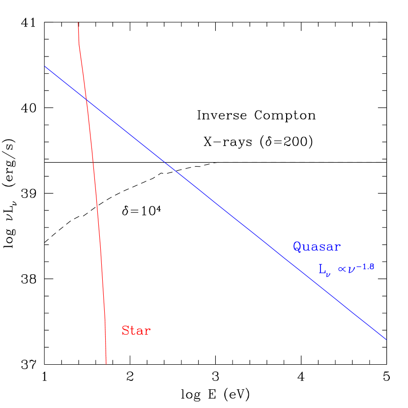
Figure 1: Comparison of stellar, QSO (with $L_{\nu}\propto\nu^{-1.8}$) and inverse Compton spectral energy distributions, all of which are normalised to have the same luminosity above 1 Ry. The inverse Compton SED is significantly harder than all others. At high densities (overdensities $\delta\sim 10^{4}$ at $z\sim 9$), cooling of relativistic electrons by ionization losses becomes significant, causing the downturn of the spectrum at low energies.

where $N(\gamma)$ is the electron energy spectrum, $J(\nu)=B_{\nu}(T_{CMB,o}(1+z))$ is the CMB blackbody spectrum, and $F(x)=1+x+2x{\rm ln}(x)-2x^{2}$. This differs only by a normalization correction from assuming that all photons reside at the peak of the blackbody spectrum, $\nu=1.6\times 10^{11}(1+z)$Hz. This is because the seed photon spectrum is narrow compared to the electron energy distribution. In figure (1), I show example spectra computed with equations (15) and (16). Note that the efficiency of Coulomb cooling depends on the assumed electron density; I assume that $n_{e}\sim\delta n_{o}(1+z)^{3}$, where I assume the overdensity to be either $\delta\sim 200$ (to mimic the overdensity at the virial radius) or $\delta\sim 10^{4}$ (to mimic the overdensity for collapsed gas in dense star forming regions). At $z\sim 10$, this assumption corresponds to $n_{e}\sim 4\times 10^{-2}\,{\rm cm^{-3}}$ and $n_{e}\sim 2\ {\rm cm^{-3}}$ respectively. Also plotted for reference is the spectrum of the same starburst with a Salpeter IMF, assuming an escape fraction of $\sim 1\%$, and the spectrum of a mini-quasar with spectrum $L_{\nu}\propto\nu^{-1.8}$, normalized to have the same energy release above the Lyman limit as the starburst. Note that the inverse Compton case has the hardest spectrum of all. Since the spectrum is so hard, photoelectric absorption by the host galaxy does not significantly attenuate the ionizing flux. Most UV photons produced will not escape the host galaxy, whereas X-ray photons with $E>270\left(\frac{N_{HI}}{10^{21}cm^{-2}}\right)\,{\rm eV}$ where $N_{HI}$ is the column density in the host galaxy, will escape unimpeded. Since $\nu L_{\nu}\sim{\rm const}$, most of the energy in ionizing photons escape. Note, incidentally, that the escape fraction for UV photons produced by inverse Compton may be significantly higher than photons of the same frequencies produced by stars, as relativistic electrons can disperse from the star forming region, where gas densities are highest and most photon captures take place.

2.4 Zero-metallicity star formation

The stellar IMF at high redshift under conditions of low or zero metallicity is unknown. Up to now, I have assumed a Salpeter IMF, in which one supernova expodes for every $\sim 100\,M_{\odot}$ of stars formed, and each supernova deposits on average $\sim 10^{50}\left(\frac{\epsilon}{0.1}\right)$erg in relativistic electrons and $\sim 1\,M_{\odot}$ of metals. Since the estimated amount of star formation at high redshift is calibrated to the observed IGM metallicity at $z\sim 3$, it is worth asking whether the energy injected into X-rays per solar mass of metals produced, $\epsilon_{Z}\sim 10^{50}\,{\rm erg\,M_{\odot}^{-1}}$, could change significantly at high redshift. I have argued that variations in the IMF will not effect significant changes in $\epsilon_{Z}$ or the ratio of energy emitted in stellar UV ionizing photons to inverse-Compton X-rays, since the same massive OB stars which produce UV ionizing photons also explode as supernova, producing both relativistic electrons and metals.

However, zero-metallicity star formation may result in very different stellar populations from that seen at low redshift. The lack of efficient cooling mechanisms could result in extremely top heavy stellar IMFs (Larson 1998, Larson 1999) and in particular the production of “Very Massive Objects” (VMOs) in the range $10^{2}-10^{5}\,M_{\odot}$ (Carr, Bond & Arnett 1984). Such stars have high effective temperatures and produce a much harder spectrum than ordinary stars (Tumlinson & Shull, 2000, Bromm et al, 2000). Moreover, the distribution of stellar endpoints is very different from a normal IMF (Heger, Woosley & Waters 2000). Stars with masses between 10 and 35 $M_{\odot}$ explode as type II supernovae. While it is not known whether metal free stars with masses between 35 and 100 $M_{\odot}$ will explode–they might collapse to form black holes–stars with masses $\sim 100-250M_{\odot}$ are disrupted by the pair production instability, once again producing an energetic supernova event and dispersing metals. Stars more massive than $250M_{\odot}$ should collapse completely to black holes, without ejecting any metals (unless they eject their envelopes during hydrogen shell burning, in which case it is possible for them to explode). The latter provides an obvious mechanism for seeding supermassive black holes to form AGN. A number of studies of zero-metallicity star formation suggest that the Jeans/Bonner-Ebert mass and hence the lower mass cutoff for star formation is very high, $M_{*}>10^{2}-10^{3}\,M_{\odot}$ (Abel, Bryan & Norman 1999, Padoan, Nordlund & Jones 1997).

There are three main observations to make: (i) VMOs with initial stellar masses $100M_{\odot}<M<250M_{\odot}$ which are disrupted by the pair-production stability show $\epsilon_{Z}(PP)\approx\epsilon_{Z}({\rm type\ II})$, which imply that even if these objects are abundant in the early universe, our estimates of the level of inverse Compton X-ray emission do not change strongly. In particular, $E_{\rm explosion}=6.3\times 10^{52}\left(\frac{M}{10^{2}M_{\odot}}\right)^{2.8}\frac{{\rm min}[0.13,(1-\phi_{L})^{2.8}]}{0.13}\,{\rm erg}$ while the yield in elements heavier than helium is $Z_{\rm ej}={\rm min}\left[(1-\phi_{L}),0.5\right]$, where $\phi_{L}$ is the fraction of the initial mass lost during hydrogen burning (Carr, Bond & Arnett, 1984). Thus, $\epsilon_{Z}(PP)=1.3\times 10^{50}\left(\frac{M}{10^{2}M_{\odot}}\right)^{1.8}\frac{{\rm min}[0.25,(1-\phi_{L})^{1.8}]}{0.25}\,{\rm erg\ M_{\odot}^{-1}}\approx\epsilon_{Z}({\rm type\ II})$. (ii) Stars which directly collapse to form black holes represent an additional, unaccounted source of ionizing photons, since they are not included in the metal pollution budget (of course, their most important contribution could lie in seeding AGN formation). (iii) Zero metallicity is a singularity: true zero-metallicity stellar populations differ greatly from low metallicity ones. Even the introduction of trace amounts of metals $Z\sim 10^{-4}Z_{\odot}$ introduces important changes in stellar structure and evolution (Heger, Woosley & Waters 2000). Furthermore, trace amounts of metals drastically reduces the abundance of VMOs by allowing efficient cooling past the 300K barrier imposed by ${\rm H}_{2}$ cooling, reducing the Jeans mass and thus the minimum mass for star formation. Prompt initial enrichment is quite plausible: the lifetime of massive stars before they explode to pollute the IGM with metals is $\sim 10^{6}$ years, which is a short fraction of the Hubble time $t_{H}\sim 8\times 10^{8}(\frac{1+z}{10})^{-3/2}$yrs even at high redshift. Although the degree of metal mixing is uncertain (e.g. Gnedin & Ostriker 1997, Nath & Trentham 1997, Ferrara, Pettini & Shchekinov 2000), note that first star forming regions are very highly biased, and subsequent generations of the halo hierarchy collapse in proto-clusters and filaments very close to the first star clusters. Thus, stars of finite metallicity could quickly predominate, even if the mean metallicity of the universe is close to primordial (Cen & Ostriker 1999). It is therefore possible and even likely that true zero metallicity star formation was confined to a very small fraction of the stars formed at high redshift, and thus negligible in terms of the energy budget for reionization.

3 Observational signatures

In this section, to estimate number counts I use the Press-Schechter based high redshift star formation models of Haiman & Loeb (1997), which are normalised to the observed metallicity of the z=3 IGM, ${\rm Z=10^{-3}-10^{-2}Z_{\odot}}$. In these models, in every halo capable of atomic cooling (i.e., with a virial temperature $T_{vir}>10^{4}$K), a fixed fraction of the gas $f_{star}=1.7,17\%$ (for ${\rm Z}(z=3)=10^{-3},10^{-2}{\rm Z_{\odot}}$ respectively) fragments in a starburst lasting $t_{o}\sim 10^{7}$yrs. The correspondence between halo mass and star formation rate is thus ${\rm SFR}\approx 2\left({\rm\frac{M_{halo}}{10^{9}\,M_{\odot}}}\right)\left(\frac{f_{star}}{0.17}\right)\ {\rm M_{\odot}\,yr^{-1}}$, and each halo is only visible for some fraction of the time $\frac{t_{o}}{t_{H}(z)}$.

3.1 HeII recombination lines

One possible signature of the hard spectrum produced by inverse Compton X-rays would be HeII recombination lines from the host galaxy. Indeed, such lines may well be detectable from the first luminous objects with sufficiently hard spectra, such as mini-quasars or metal-free stars (Oh, Haiman & Rees 2000). The different sources may perhaps be distinguished on the basis of line widths and line ratios (Tumlinson, Giroux & Shull, 2000). However, inverse Compton emission produces too few HeII ionizing photons for such recombination lines to be detectable with NGST at high redshift. For a Salpeter IMF, $\dot{N}_{ion,HI}=10^{53}{\rm\left(\frac{SFR}{1M_{\odot}\,yr^{-1}}\right)}\ {\rm photons\,s^{-1}}$ from stellar UV radiation. On the other hand, since secondary ionizations of HeII are negligible (Shull & van Steenberg 1985), the production rate of HeII ionizing photons from non-thermal emission is $\dot{N}_{ion,HeII}=\int_{4\nu_{L}}^{\nu_{thin}}\frac{L_{\nu}}{h\nu}\approx 2.5\times 10^{49}\left(\frac{SFR}{1\,M_{\odot}\,yr^{-1}}\right)\ {\rm photon\,s^{-1}}$, where $\nu_{thin}$ is the frequency at which the halo becomes optically thin. Thus, $Q\equiv\dot{N}^{\rm HeII}_{\rm ion}/\dot{N}^{\rm HI}_{\rm ion}\approx 2.5\times 10^{-4}$, as compared with $Q\approx 0.05$ for stellar emission from metal-free stellar population, and $Q\approx 4^{-\alpha}=0.08-0.25$ for a QSO, where $L_{\nu}\propto\nu^{-\alpha}$ and $\alpha=1-1.8$, implying that the relative flux in HeII and H$\alpha,\beta$ recombination lines is much smaller for inverse Compton emission than metal-free stars or AGN. The luminosity in a helium recombination line $i$ may be estimated as $L_{\rm i}=Qf_{\rm i}L_{\rm H\alpha}$, where $L_{\rm H\alpha}$ is the Balmer $\alpha$ line luminosity, $f_{\rm i}\equiv\frac{j_{i}}{j_{H\alpha}}\left(\frac{\alpha_{B}(HI)n_{HII}}{\alpha_{B}(HeII)n_{HeIII}}\right)$, $\epsilon$ is the fraction of SN energy which emerges as IC emission, and $j_{i},j_{H\alpha}$ may be obtained from Seaton (1978). The observed flux is $J_{i}=\frac{L_{\rm i}}{4\pi d_{\rm L}^{2}}\frac{1}{\delta\nu}=0.04\left(\frac{q_{\rm i}}{0.5}\right)\left(\frac{1+z}{10}\right)^{-1}\left(\frac{\epsilon}{0.1}\right)\left(\frac{R}{1000}\right)\left(\frac{{\rm SFR}}{1{\rm M_{\odot}yr^{-1}}}\right)\,{\rm nJy}$ where ${\rm R}$ is the spectral resolution, and $q_{\rm i}\equiv f_{\rm i}\nu_{\rm H\alpha}/\nu_{\rm i}$, where $f_{\lambda 4686}=0.74,f_{\lambda 1640}=4.7,f_{\lambda 3203}=0.30$. This is undetectable by NGST, which in $10^{5}$s integration time requires for a 10 $\sigma$ detection a flux $F(10\sigma)\sim 30$nJy at these frequencies (observed wavelengths $1<\lambda<5.5\mu$m) and spectral resolution $R\sim 1000$ (see Oh, Haiman & Rees 2000 for details).

It is worth mentioning that a hard source may produce relatively little recombination line flux and yet play an important role in reionizing the universe. The recombination line flux from a source is $\propto(1-f_{esc})$, whereas the ionizing flux escaping into the IGM is $\propto f_{esc}$ (where $f_{esc}$ is significantly higher for hard sources: all photons with $E>E_{halo,thin}=270\left(\frac{N_{HI}}{10^{21}{\rm cm}^{-2}}\right)$eV can escape freely from the host). Secondary ionizations are unimportant within a host halo: much of the gas in fully ionized, in which case the energetic photoelectron deposits its energy as heat. In any case, the halo is optically thin to the most energetic photons $E>E_{halo,thin}$ which are important for secondary ionizations. Thus, in recombination line flux what matters is the total number of ionizing photons produced, whereas for the reionization of the IGM what matters is the total output energy (since in a largely neutral medium with $x_{e}<0.1$ the total number of ionizations for a photon of energy $E_{photon}$, including secondary ionizations, is $N_{ion}\sim E_{photon}/37{\rm eV}$ (Shull & van Steenberg 1985). Note, however, that as the medium becomes more ionised an increasing fraction of the energy is deposited as heat, and an additional source of soft photons is needed for reionization to proceed (Oh 2000a)). Thus, for instance, for $f_{esc}\sim 1\%$, inverse Compton radiation makes a negligible contribution to the H$\alpha$ luminosity, $\frac{L_{H\alpha}^{IC}}{L_{H\alpha}^{stellar}}\approx\frac{\dot{N}_{ion}^{IC}}{\dot{N}_{ion}^{stellar}}=2.5\times 10^{-4}$, but the ionizing IC and stellar radiation escaping from the host are energetically comparable (from equations (1) and (3), $L_{X}^{IC}\approx L_{UV}^{stellar}$), and thus they produce roughly equal number of ionizations in the IGM.

3.2 X-rays and gamma-rays

Unfortunately, direct detection of inverse Compton X-rays from high-redshift star clusters is unlikely. From equation (1), the observed flux in X-rays from a star forming region is:

$$f=\frac{L}{4\pi d_{L}^{2}}=5\times 10^{-20}\left(\frac{\epsilon}{0.1}\right)\left(\frac{\rm SFR}{1{\rm M_{\odot}yr^{-1}}}\right)\left(\frac{1+z}{10}\right)^{-2}\,{\rm erg\,s^{-1}\,cm^{-2}}$$ (17)

By contrast, the Chandra X-ray Observatory (CXO) sensitivity (see http://chandra.harvard.edu/) for a 5$\sigma$ detection of a point source in an integration time of $10^{5}$s in the 0.2–10 keV range is $F_{X}=4\times 10^{-15}\,{\rm erg\,s^{-1}\,cm^{-2}}$. The next generation X-ray telescope, Constellation-X (http://constellation.gsfc.nasa.gov/) is optimised for X-ray spectroscopy and will not have significantly greater point source sensitivity: for a similar bandpass and integration time it will be able to detect objects out to a flux limit of $F_{X}=2\times 10^{-15}\,{\rm erg\,s^{-1}\,cm^{-2}}$. Thus, in a week CXO and Constellation-X will at best be able to detect starbursts (with seed photons provided by the IR radiation field from dusty star forming regions) with star formation rates SFR $\sim 100\,{\rm M_{\odot}yr^{-1}}$ (corresponding to $L_{X}\sim 4.8\times 10^{42}\,{\rm erg\,s^{-1}}$) out to redshift $z\sim 1$ (note that the Lyman-break galaxies detected at $z\sim 3$ (Steidel et al 1996) typically have have inferred star formation rates ${\rm SFR}\sim 100{\rm M_{\odot}\,yr^{-1}}$), while the very brightest starbursts, with star formation rates of SFR$\sim 1000\,{\rm M_{\odot}yr^{-1}}$, might be detectable out to $z\sim 3$. As discussed in section 3.4, simultaneous detection of synchrotron radiation with the Square Kilometer Array will then constrain magnetic field strengths in these objects.

Detection in gamma ray emission is also unlikely. The upcoming Gamma-ray Large Area Space Telescopy (GLAST) (http://glastproject.gsfc.nasa.gov/) will have a flux sensitivity of $\sim 2\times 10^{-9}{\rm photons\,cm^{-2}\,s^{-1}}$ in the 20MeV–300GeV range, whereas star-forming regions at high redshift will have fluxes of at most $F_{\gamma}\sim 10^{-15}\left(\frac{\epsilon}{0.1}\right){\rm\left(\frac{SFR}{1M_{\odot}\,yr^{-1}}\right)}\left(\frac{1+z}{10}\right)^{-2}{\rm photons\,cm^{-2}s^{-1}}$.

What fraction of the unresolved X-ray and gamma-ray background could be due to star formation at high redshift $z>3$? Observations of absorption in CIV and other metals in Ly$\alpha$ forest absorption lines with $10^{14.7}{\rm cm^{-2}}<N_{HI}<10^{16}{\rm cm^{-2}}$ indicate that $Z\sim 10^{-2}Z_{\odot}\sim 2\times 10^{-4}$. Each supernova produces about $\sim 1M_{\odot}$ of metals (Woosley & Weaver 1995). Assuming $(\Omega_{b},h)=(0.04,0.65)$, this implies one supernova every $\sim 1000\,{\rm kpc^{3}}$ (comoving). If each supernova injects $\sim 10^{50}$ ergs in hard X-rays, the comoving X-ray energy density was $U_{X}\sim\frac{c}{4\pi}\frac{U_{X}}{(1+\bar{z})}\sim 2\times 10^{-6}{\rm eV\,cm^{-3}}$. If the mean source redshift was $\bar{z}\sim 5$, the distant sources produced a diffuse flux of $J\sim 1{\rm keVs^{-1}cm^{-2}sr^{-1}}$. One can make a more detailed estimate using the equation of cosmological transfer (Peebles 1993):

$$J(\nu_{o},z_{o})=\frac{1}{4\pi}\int_{z_{o}}^{\infty}dz\frac{dl}{dz}\frac{(1+z_{o})^{3}}{(1+z)^{3}}\epsilon(\nu,z)e^{-\tau_{{\rm eff}}(\nu_{o},z_{o},z)}$$ (18)

where $z_{o}$ is the observer redshift, $\nu=\nu_{o}(1+z)/(1+z_{o})$, and $\epsilon(\nu,z)$ is the comoving X-ray emissivity. Using the star formation model of Haiman & Loeb (1997), I obtain the estimate:

$$\nu J_{\nu}=0.8\left(\frac{\epsilon}{0.1}\right)\left(\frac{Z(z=3)}{10^{-2}Z_{\odot}}\right){\rm keV\,s^{-1}cm^{-2}sr^{-1}}\ \ {\rm for}\ z_{source}\geq 3$$ (19)

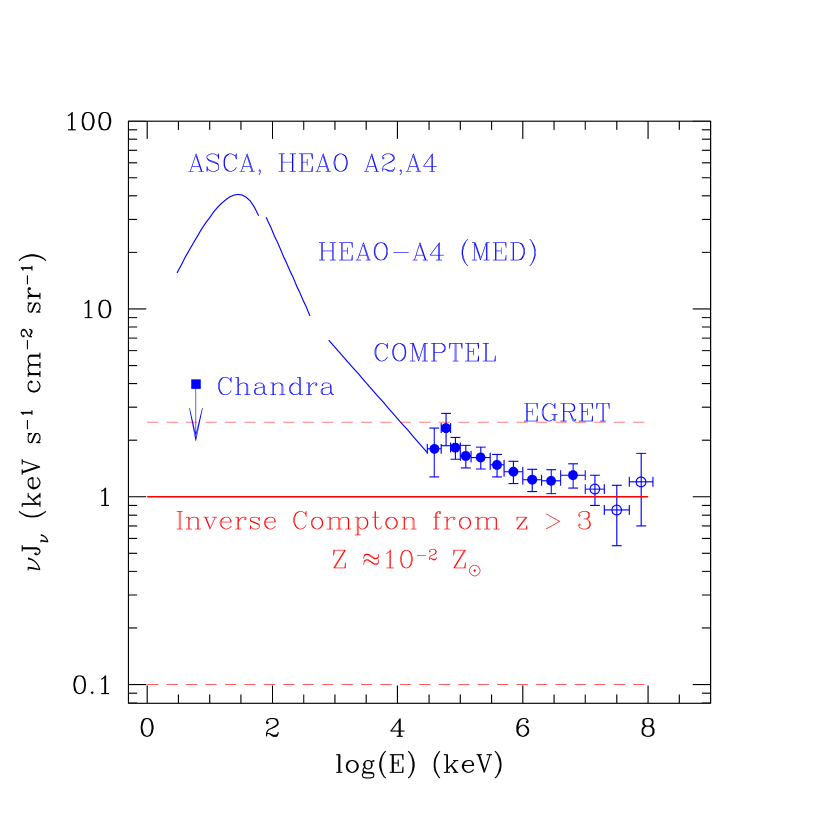
Figure 2: Current best observational limits on the X-ray and gamma-ray background, against model predictions. The solid line represents model predictions for an IGM metallicity at z=3 of ${\rm Z\approx 10^{-2}Z_{\odot}}$, while the upper and lower dotted lines represent generous limits of ${\rm Z\approx 2.5\times 10^{-2}Z_{\odot}}$ and ${\rm Z\approx 10^{-3}Z_{\odot}}$ respectively. Note that inverse Compton radiation from high redshift can account for the majority of the observed gamma-ray background.

In Fig (2), I display this predicted level of emission against the observed X-ray and gamma-ray background in the 1 keV –100 GeV range, from analytic fits to the ASCA and HEAO A2,A4 data in the 3-60 keV range (Boldt 1987), the HEAO 1 A-4 data in the 80-400 keV range (Kinzer et al 1997), the COMPTEL data in the 800 keV – 30MeV range (Kappadath et al 1996). Data points from EGRET in the 30 MeV – 100 GeV range (Sreekumar et al 1998) are also shown. The level of the unresolved background of course depends on the sensitivity of the instrument; recently CXO resolved $\sim 80\%$ of the hard X-ray background in the 2-10 keV range into point sources (Mushotzky et al 2000). This agrees well with the predictions of XRB synthesis models (e.g., Madau, Ghisellini & Fabian 1994), which use AGN unification schemes to reproduce the observed spectral shape of the XRB. A prediction of the IC scenario presented here is that a non-trivial fraction of the X-ray/gamma-ray background will not be resolved into point sources with upcoming missions, due to the extreme faintness of high redshift sources.

It is particularly intriguing that both the amplitude and spectral shape of the gamma-ray background as observed by EGRET is well-matched by the predicted level of gamma-ray emission in this model. This raises the exciting possibility that the majority of the observed gamma-ray background comes from inverse Compton emission at high redshifts. At present, the origin of the gamma-ray background is still unknown. The most favoured scenario for some time was that it is due to unresolved gamma-ray blazars (Bignami et al 1979, Kazanas & Protheroe 1983, Stecker & Salamon 1996): the observed blazar $\gamma$-ray spectrum has an average spectral index compatible with the observed GRB (Chiang & Mukherjee 1998). However, extrapolation of the observed EGERT blazar luminosity function implies that unresolved blazars can account for at most $\sim 25\%$ of the diffuse $\gamma$-ray background (Chiang & Mukherjee 1998). The unresolved blazar model will most likely be decisively tested by GLAST (Stecker & Salamon 1999), which will be two orders of magnitude more sensitive than EGRET. A host of other models include pulsars expelled into the halo by asymmetric supernova explosions (Dixon et al 1998, Hartmann 1995), primordial black hole evaporation (Page & Hawking 1976), supermassive black holes at very high redshift (Gnedin & Ostriker 1992), annihilation of weakly interactive big bang remnants (Silk & Srednicki 1984, Rudaz & Stecker 1991) and finally, inverse Compton radiation from cosmic ray electrons in our own Galaxy (Strong & Moskalenko 1998, Dar & De Rujula 2000), and from collapsing clusters (Loeb & Waxman 2000). However, to date the possibility of inverse Compton emission from high redshift supernovae has not been discussed.

A scenario in which the majority of the gamma-ray background comes from inverse Compton emission at high redshift make a number of firm predictions: (i) As previously mentioned, the majority of the GRB will remain unresolved by GLAST, due to the extreme faintness of the contributing sources. (ii) After removal of the Galactic contribution, which is correlated with the structure of our Galaxy and our position within it (Dixon et al 1998, Dar et al 1999), a highly isotropic component of the GRB will still be present. (iii) The GRB should be extremely smooth, and exhibit significant fluctuations only at extremely small angular scales. The fluctuations should be dominated by the Poisson rather than the clustering contribution (see Oh 1999). Using $\langle S^{n}\rangle=\int_{0}^{S_{c}}\frac{dN}{dS}S^{n}$, where $S_{c}$ is the cut-off flux for point source removal, and the star formation model of Haiman & Loeb (1997), I find that for $z>3$ sources (which are too faint to be removed as point sources), $\frac{\langle I^{2}\rangle^{1/2}}{\langle I\rangle}=3.4\times 10^{-2}\left(\frac{\theta}{5^{\prime}}\right)^{-1}$, where $I$ is surface brightness (the angular resolution of GLAST is expected to be of order $1-5$ arcmin). (iv) The gamma-ray background at $E>100$GeV should be attenuated, due to pair production opacity against IR/UV photons (e.g., Salamon & Stecker 1998, Oh 2000b). High energy photons initiate an electromagnetic cascade which transfers energy from high energy photons to the lower energy portion of the spectrum, where the universe is optically thin (Coppi & Aharonian 1997). Note that the EGRET spectrum was directly determined with data only up to 10 GeV; beyond 10 GeV larger uncertainties exist due to backsplash in the NaI calorimeter, and Monte-Carlo simulations were used to determine the differential flux in the 10-30,30-50 and 50-120 GeV range (Sreekumar et al 1998). Thus, the EGRET data points with $E>10$GeV are less reliable. It would be intriguing to see if GLAST (sensitive out to 300 GeV) indeed shows an absorption edge to the gamma-ray background at higher energies. It would also be interesting to look for absorption of the gamma-ray background in a line of sight passing through a massive cluster (indicating that the gamma-rays come from higher redshifts than the cluster); the pair-production optical depth through a cluster is of order $\tau\sim 2n_{\gamma}\sigma_{T}r_{vir}\sim 0.4$ (assuming $n_{\gamma}\sim 0.1{\rm cm^{-3}}$ and $r_{vir}\sim 1$Mpc).

3.3 CMB constraints

Will the upscattering of CMB photons by relativistic electrons at high redshift produce an observable signal in the CMB, or violate any present observational constraints? When the electrons are relativistic, CMB photons are inverse Compton scattered to such high energies (completely out of the detector bandpass) the process may simply be thought of as absorption, $\delta I/I\sim\tau_{e}^{rel}$, where $\tau_{e}^{rel}$ is the optical depth of relativistic electrons, and $I$ is the number flux of CMB photons. The flux decrement due to the absorption of CMB photons may be estimated as:

$$\Delta S_{\nu}\approx J_{CMB}\int d\Omega\int dln_{e}^{rel}\sigma_{T}=J_{CMB}\sigma_{T}\frac{N_{e}^{rel}}{d_{A}^{2}}$$ (20)

where $J_{CMB}$ is the blackbody surface brightness of the CMB, and $N_{e}^{rel}$ is the total number of relativistic electrons in the system. The steady state number of relativistic electrons is given by $N_{e}^{rel}=\int d\gamma N(\gamma)$ where $N(\gamma)$ is given by equation (15). Since the CMB flux peaks at $\nu\sim 10^{11}$Hz, the absolute magnitude of the flux decrement is maximized by going to similar frequencies. At 20 GHz, the highest frequency detectable by SKA, the SKA has an rms sensitivity of $\sim 6$nJy for a $10^{5}$s integration. On the other hand, the flux decrement is $\Delta S_{\nu}(20\,{\rm GHz})\sim 3.5\times 10^{-5}(\frac{1+z}{10})^{2}(N_{e}^{rel}/3\times 10^{58}{\rm electrons})$ nJy, which is unobservably small.

One might hope to detect the mean signal of all the CMB photons upscattered by relativistic electrons. In particular, since the number of CMB photons is no longer conserved, the absorption might be detectable as a chemical potential distortion of the CMB. Let us estimate the number of CMB photons destroyed. Each supernova upscatters at most $N_{scattered}\sim\epsilon E_{SN}/\langle E_{X}\rangle\sim 10^{60}$ CMB photons, where I have set the average photon energy $\langle E_{X}\rangle\sim 100$eV (note that since the number of photons $N_{\nu}\propto\nu^{-1}$, most of the upscattered photons are of low energy). For a metallicity of $Z\sim 10^{-2}Z_{\odot}$ at $z\sim 3$, one supernova has gone off every comoving $V_{SN}\sim 1000\,{\rm kpc^{3}}$, and thus the comoving number density of upscattered CMB photons is $\delta n\sim N_{scattered}/V_{SN}\sim 4\times 10^{-8}\,{\rm cm^{3}}$. Since $n_{\gamma}\sim 400\,{\rm cm^{-3}}$, we have $\delta n/n\sim 10^{-10}$, which results in an undetectably small chemical potential distortion. Thus, the upscattering of CMB photons at high redshift does not violate any distortion constraints on the CMB.

If the IGM is reionized inhomogeneously, as in canonical models, then secondary CMB anistropies will be created by CMB photons Thompson scattering off moving ionized patches (Agahanim et al 1996, Grusinov & Hu 1998, Knox et al 1998). The power spectrum is generally white noise, with $\Delta T/T\sim 10^{-6}-10^{-7}$, peaking at arc-minute to sub arc-minute scales. However, if the IGM is reionized fairly homogeneously by X-rays then over a line of sight the positive and negative contributions of the velocity field will cancel out. In this case, only the second-order Ostriker-Vishniac effect due to coupling between density and velocity fields will be present. A null detection of the inhomogeneous reionization anisotropy could place upper limits on the patchiness of reionization, although this will be a difficult measurement as the inhomogeneous reionization and Ostriker-Vishniac signals are likely to be of comparable strength (Haiman & Knox 1999).

3.4 Radio observations

The supernovae that exploded generate magnetic turbulence and magnetic fields, which allow Fermi acceleration to take place (Jones & Ellison 1991, Blandford & Eichler 1987); observations of local radio galaxies in non-thermal radio and X-ray emission yield field strengths consistent with equipartition between relativistic particles and the magnetic field (Kaneda et al 1995). If such magnetic fields are present in the first star clusters, the relativistic electron population is a source of synchrotron radio emission as well as inverse-Compton emission. Below I find that for a given relativistic electron population, the Square Kilometer Array (SKA) will be much more sensitive to non-thermal radio emission than CXO or Constellation-X will be to inverse Compton X-ray emission. Radio observations will thus allow one to establish the presence of relativistic electrons in objects too faint to observe directly in X-ray emission. Since one knows the CMB energy density exactly as a function of redshift, given reasonable assumptions for the magnetic field the observed radio emission allows one to immediately estimate the amount of inverse Compton X-ray emission which must be taking place,

$${\rm L_{X}}=\frac{\rm U_{CMB}(z)}{\rm U_{B}}{\rm L}_{\rm synch}$$ (21)

The transition Lorentz factor $\gamma_{break}$ at which electron energy losses are dominated by inverse Compton rather than ionization losses is given by equation (9). Above an observed radio frequency $\nu_{break}=\nu_{L}\gamma_{break}^{2}/(1+z)=2.8\times 10^{4}{\rm\left(\frac{B}{10\mu G}\right)}\left({\rm\frac{{\rm n}}{1\,{\rm cm^{-3}}}}\right)\left(\frac{1+z}{10}\right)^{-5}$ Hz (where $\nu_{L}\equiv\frac{eB}{2\pi m_{e}c}$ is the electron gyrofrequency), the steady state electron population is determined by balance between supernova injection and inverse Compton losses, and is given by equation (15). From standard formulae for synchrotron emissivity (Rybicki & Lightman 1979) $\epsilon_{\nu}^{synch}=\sigma_{T}\gamma^{2}\beta^{2}U_{mag}c\,{\rm n(E)dE/d\nu}$ (where n(E) is the number density of emitting electrons in $dE$) this yields a synchrotron luminosity:

$$L_{\nu}^{sync}=2.7\times 10^{28}{\rm\left(\frac{B}{10\mu G}\right)}^{1+\alpha}\left(\frac{\nu}{1\,{\rm GHz}}\right)^{-\alpha}{\rm\left(\frac{SFR}{1M_{\odot}\,yr^{-1}}\right)}\left(\frac{\epsilon}{0.1}\right)f(z,U_{\gamma})\ {\rm erg\,s^{-1}Hz^{-1}}$$ (22)

where $f(z,U_{\gamma})={\rm min}\left[\left(\frac{1+z}{10}\right)^{-4},\left(\frac{U_{\gamma}}{4.2\times 10^{-9}\,{\rm erg\,cm^{-3}}}\right)^{-1}\right]$ (the latter term in brackets is used if the stellar radiation field has a higher energy density than the CMB). By contrast, the thermal free-free emission is given by (Oh 1999):

$$L_{\nu}^{ff}=1.2\times 10^{27}\left(\frac{{\rm SFR}}{1{\rm M_{\odot}yr^{-1}}}\right)\ {\rm erg\,s^{-1}\,Hz^{-1}}$$ (23)

Thus, assuming $\alpha=1$, at observed frequencies $\nu<\nu_{trans}=2.3\left(\frac{1+z}{10}\right)^{-1}{\rm\left(\frac{B}{10\mu G}\right)}^{2}\left(\frac{\epsilon}{0.1}\right)f(z,U_{\gamma})\,{\rm GHz}$ synchrotron emission dominates over free-free emission. This is well within the 0.1–20 GHz capability of the SKA. However, this is only true if the power law for electron population extends to high energies. If it is truncated at some maximum Lorentz factor $\gamma_{max}$, then synchrotron emission is only observable for $\nu<\nu_{max}=\nu_{L}\gamma^{2}_{max}=0.28\left(\frac{1+z}{10}\right)^{-1}{\rm\left(\frac{B}{10\mu G}\right)}\left(\frac{\gamma_{max}}{10^{4}}\right)^{2}\,{\rm GHz}$. If $\nu_{max}<\nu_{trans}$, this will be manifested by an abrupt drop in radio flux at $\nu_{max}$, beyond which the emission takes the flat spectrum free-free emission form (this does not take place for expected values of $\gamma_{max}=7.4\times 10^{6}{\rm\left(\frac{B}{10\mu G}\right)}^{1/2}\left(\frac{v_{sh}}{2000\,{\rm km\,s^{-1}}}\right)\left(\frac{1+z}{10}\right)^{-2}$; see equation (13)). Observation of such a drop will yield valuable constraints on $B,\gamma_{max}$ in the first objects; the value of $\gamma_{max}$ in turn constrains the upper energy cutoff in the inverse Compton X-ray/gamma-ray spectrum, which could be important in determining whether high-redshift starbursts make a significant contribution to the gamma-ray background.

Can radio emission from star clusters at high redshift be detected by the proposed Square Kilometer Array? Non-thermal emission can be distinguished from free-free emission with multi-frequency observations to identify frequency regimes where the spectral slope is steep.The SKA detector noise may be estimated as:

$$S_{\rm instrum}=\frac{2kT_{\rm sys}}{A_{\rm eff}\sqrt{2t\Delta\nu}}=25\left(\frac{\Delta\nu}{160\,{\rm MHz}}\right)^{-1/2}\left(\frac{t}{10^{5}\,s}\right)^{-1/2}{\rm nJy}$$ (24)

where I have used $A_{\rm eff}/T_{\rm sys}=2\times 10^{8}{\rm cm^{2}/K}$ for the SKA (Braun et al 1998), and I assume a bandwidth $\Delta\nu\approx 0.5\nu$. The flux density due to non-thermal emission from a high-redshift star cluster, assuming $\alpha=1$, is:

$$S_{\nu_{o}}=\frac{L_{\nu}(\nu_{o}(1+z)}{4\pi d_{L}^{2}}(1+z)=8.5{\rm\left(\frac{B}{10\mu G}\right)}^{1+\alpha}\left(\frac{\nu}{320MHz}\right)^{-\alpha}{\rm\left(\frac{SFR}{1M_{\odot}\,yr^{-1}}\right)}\left(\frac{\epsilon}{0.1}\right)\left(\frac{1+z}{10}\right)^{-2}f(z,U_{\gamma}){\rm nJy}$$ (25)

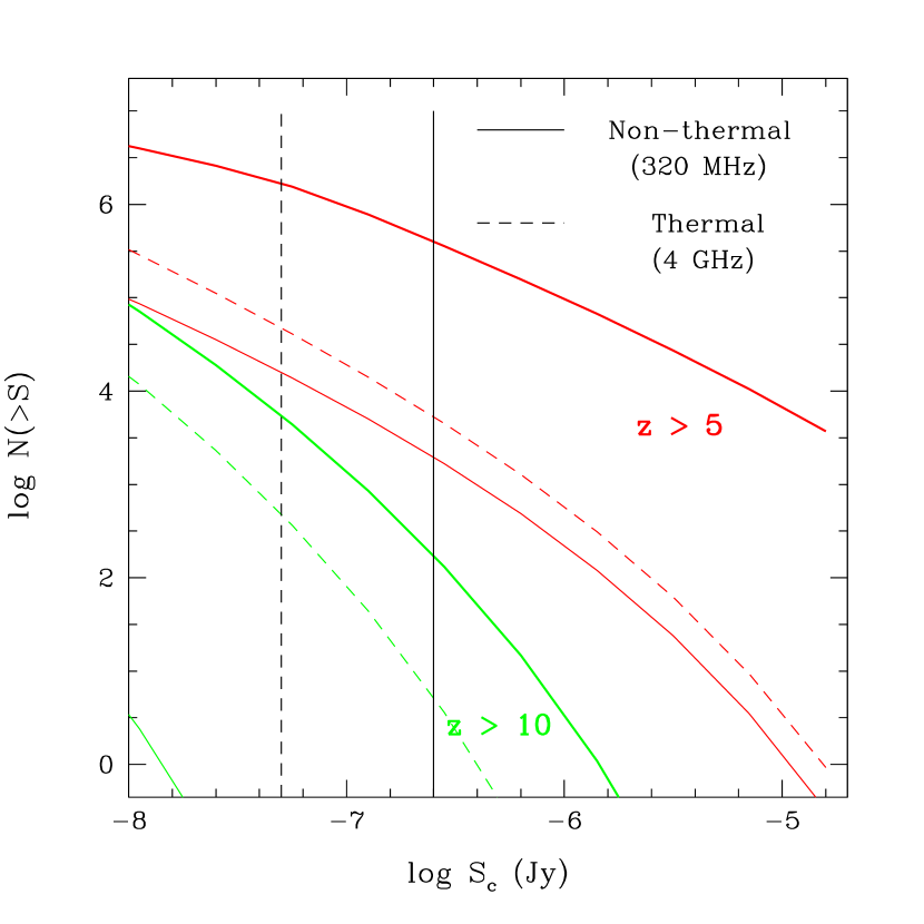
Figure 3: Number of objects with $z>5,z>10$ detectable in non-thermal emission in the $1^{\circ}$ field of view of the SKA at 320 MHz; the limiting flux for a 10 $\sigma$ detection in a $10^{5}$s integration is displayed as a solid line. The dark solid line is for an efficiency factor $f_{radio}={\rm\left(\frac{B}{10\mu G}\right)}^{1+\alpha}\left(\frac{\epsilon}{0.1}\right)\left(\frac{f_{star}}{0.17}\right)=1$, the light solid line is for $f_{radio}=10^{-2}$. Also shown as dotted lines is the detection rate and limiting flux at 4 GHz, when free-free emission is dominant, for a high efficiency star formation model ($f_{star}=17\%$).

Thus, a source with SFR$\sim 10{\rm M_{\odot}yr^{-1}}$ at $z\sim 9$ can be detected as a 10$\sigma$ detection in 10 days. To estimate the number of sources detectable by SKA, I use the Press-Schechter based high redshift star formation models of Haiman & Loeb (1997), and define an efficiency factor $f_{radio}={\rm\left(\frac{B}{10\mu G}\right)}^{1+\alpha}\left(\frac{\epsilon}{0.1}\right)\left(\frac{f_{star}}{0.17}\right)$, where $f_{star}$ is the fraction of halo gas which fragments to form stars. In Figure (3), I display the number of sources above a given redshift which may be detected in non-thermal emission in the $1^{\circ}$ SKA field of view, assuming $f_{radio}=1,0.01$. Also shown is the number of sources which can be detected in free-free emission at 4 GHz. One should be able to detect a large number of sources at high redshift, $z>5$. Thus, radio observations of non-thermal emission can serve as a useful proxy for X-ray observations in allowing one to estimate $L_{X}$, and thus the overal level of X-ray emission at high redshift.

3.5 Multi-wavelength observations

While a detailed study of high-redshift multi-wavelength campaigns is beyond the scope of this paper, below I describe some possible follow-up observations if synchrotron emission is detected at high redshift.

• Redshift estimates Thus far the most efficient way to select high-redshift radio galaxies has proven to be the observation of steep radio spectra $\alpha<-1.3$ (Chambers et al 1990, van Breugel et al 1999). This is at least partially due to the fact that extremely bright radio galaxies have SEDs which steepen with frequency; the k-correction then implies that sources at increasing redshift have steeper observed spectra. Steepening with redshift due to inverse Compton losses, as well as selection effects (i.e., brighter sources have stronger magnetic fields, and thus more rapid synchrotron losses) could also play a role (Krolik & Chen 1991). This technique may fail for fainter sources at high redshift since for $\nu>{\rm min}(\nu_{trans},\nu_{max})$, the radio flux will be dominated by free-free emission and the spectra will appear flat. For instance, for $B<3\left(\frac{1+z}{10}\right)^{2.5}\left(\frac{\epsilon}{0.1}\right)^{0.5}\,\mu$G, we have $\nu_{trans}<160$MHz and SKA will only detect free-free emission within its frequency coverage. An efficient way to select high-redshift objects prior to reionization would be to perform broad-band deep field imaging with NGST and select Lyman-break dropouts as has been done at $z\sim 3$ (Steidel et al 1996); before the epoch of reionization one must select ’Gunn-Peterson dropouts’, i.e. galaxies with no flux shortward of rest-frame HI Ly$\alpha$. Yet another method of selecting high-redshift objects would be to perform a joint survey in the submm with the Atacama Large Millimeter Array (ALMA); at low redshift the submm dust emission scales almost linearly with other star formation indicators, such as radio and UV emission. However, for $z\approx 0.5-10$ and a given dust emission SED the K-correction almost balances the cosmological dimming of a source, implying a flux density almost independent of redshift (e.g., Blain et al 2000). This has spawned suggestions to obtain approximate redshifts by the flux density ratio between submm and radio wavebands (Carilli & Yun 1999, 2000), although uncertainties include an AGN contribution to the radio flux and the dust temperature in the galaxy, with a degeneracy between hotter galaxies at high redshift and cooler ones nearby (Blain 1999).

• Relative importance of X-ray and UV stellar emission for reionization As previously noted, from a measurement of the radio synchrotron flux we can use equation (21) to estimate the level of inverse Compton X-ray emission which must be taking place. Redshifts and thus ${\rm U_{CMB}(z)}$ can be determined with Balmer line spectroscopy with NGST, while ${\rm U_{B}}$ can be estimated by assuming a magnetic field strength required to minimise the total energy density of the system (this is close to the value for energy equipartition between relativistic particles and magnetic fields). Observations of local radio galaxies in non-thermal radio and X-ray emission yield field strengths consistent with the minimum energy value (Kaneda et al 1995). NGST can constrain the rest-frame UV emission, and a joint measurement of the rest-frame UV flux longward of Ly$\alpha$ and the Balmer line flux (where ${\rm L_{H\alpha}}\propto(1-f_{esc})\dot{N}_{ion}$) can constrain $f_{esc}$, the escape fraction of ionizing photons, where one roughly expects $J_{H\alpha}\sim 40(1-f_{esc})J_{IR}(R/1000)$. Thus, joint SKA/NGST observations could place limits on whether inverse Compton X-rays or stellar UV photons were energetically dominant and thus more important in reionizing the universe.

• Measuring magnetic fields in bright sources The very brightest sources out to $z\sim 3$ will also be visible in X-ray emission with CXO; the fact that the same population of relativistic electrons is responsible for non-thermal X-ray and radio emission can be confirmed by comparing respective spectral slopes. In this case, one can estimate the strength of magnetic fields, ${\rm U_{B}}\approx\frac{L_{X}}{L_{sync}}{\rm U_{CMB}(z)}$. Since dust obscuration is unimportant at both hard X-ray and radio wavelengths, the measurement should be fairly robust.

• Distinguishing between synchrotron emission from AGN and supernovae To confirm that such emission arises from star-forming regions rather than an AGN, one might look for signs of diffuse emission (note that the angular resolution of the SKA is $\sim 0.1^{\prime\prime}$, while the angular scale of the virial radius of typical objects will be $\theta_{vir}\sim 0.5^{\prime\prime}(M/10^{9}M_{\odot})^{1/3}$). AGNs can be selected on the basis of color, as has been successfully carried out at lower redshifts (Fan 1999), using broad band NIR and MIR imaging with NGST. Finally, the line widths of the H$\alpha$, H$\beta$ lines as observed with NGST may be considerably broader for an AGN ($\sigma\sim 1000\,{\rm km\,s^{-1}}$), due to line broadening by the accretion disc.

4 Conclusions

X-ray emission from a early star forming regions is predicted to be large and energetically comparable to UV emission. Non-thermal inverse Compton emission, which provides a good fit to local observations and should become increasingly important at high redshift, due to the evolution of the CMB energy density, is predicted to be the dominant source of X-rays. It introduces a whole host of physical consequences: the topology of reionization changes, becoming more homogeneous with much fuzzier delineation between ionized and neutral regions; reheating temperatures increase, with implications for feedback on structure formation and the observed width of Ly$\alpha$ forest lines; the abundance of free electrons in dense regions increases, promoting gas phase $H_{2}$ formation, cooling, and star formation. These effects will be considered in a companion paper (Oh 2000a). While direct detection of individual sources with CXO or Constellation-X appears difficult, we can hope to confirm the presence of relativistic electrons in high redshift objects by detecting non-thermal radio emission with the Square Kilometer Array. Given the CMB energy density at that epoch, this yields a minimal level of inverse Compton X-ray emission. Combined with NGST observations of rest frame UV emission, this will determine if stellar radiation or inverse Compton X-rays were the dominant factor in reheating and reionizing the universe. In addition, in this scenario a non-trivial fraction of the hard X-ray and gamma-ray background comes from inverse Compton emission at high redshift. In particular, it is possible to reproduce both the shape and amplitude of the gamma-ray background observed by EGRET, and predict that the majority of the smooth, isotropic gamma-ray background will remain unresolved by GLAST, which should display attenuation above $\sim 100$GeV, from the pair production opacity due to ambient UV/IR radiation fields.

Many of the conclusions in this paper depend upon a scenario in which the escape fraction of UV ionizing photons is small, $f_{esc}<10\%$. This assumption is well supported by observations in the local universe, as well as theoretical radiative transfer calculations of high redshift star forming regions, which predict very low escape fractions, $f_{esc}\sim 0.01$ (Wood & Loeb 1999, Ricotti & Shull 1999, although note that the latter authors predict a substantial escape fraction at low masses $10^{7}M_{\odot}$). However, note that the latter ignore gas clumping and the multi-phase structure of the ISM. If for some reason the escape fraction is unexpectedly high (e.g. the supernovae blow holes in the ISM through which UV photons can escape), then the X-ray component is energetically subdominant and stellar UV radiation dominates the reionization of the universe. Even in this regime, the X-ray component still plays a role in heating the gas above 15 000 K, He II reionization, and promoting gas phase ${\rm H_{2}}$ formation, as these tasks cannot be accomplished by soft photons. The escape fraction of UV ionising photons in high redshift objects may eventually be deduced by comparing the IR and $H\alpha$ fluxes observed by NGST (Oh 1999).

The most uncertain aspect of this paper is the assumed level of X-ray luminosity, $L_{X}\sim 0.1\dot{E}_{SN}$. I have calibrated the conversion rate via local X-ray and gamma-ray observations of starburst galaxies and individual supernova remnants within our galaxy, and argued that efficiency of all proposed X-ray production mechanisms either remains constant or increases with redshift. If the X-ray emission in local starbursts is primarily due to inverse Compton scattering of soft IR photons (Moran & Lehnart 1997, Moran, Lehnart & Helfand 1999), the empirical relation between star formation rate and X-ray luminosity (equation (1)) implies an electron acceleration efficiency of $\epsilon\sim 10\%$, which lies at the upper limit of theoretical expectations. If instead the empirical relation (1) is approximately correct but the X-rays arise from a variety of emission mechanisms, the importance of X-rays for reionization still holds, but specific observational tests which rely on the inverse-Compton mechanism, such as the gamma-ray background observations(section (3.2)) and observations of radio synchrotron emission with the SKA (section (3.4)) will fail.

5 Acknowledgements

I am very grateful to my advisor David Spergel for his encouragement and advice. I also thank Roger Blandford, Andrea Ferrara, Zoltan Haiman and Ed Turner for helpful conversations, and Bruce Draine and Michael Strauss for detailed and helpful comments on an earlier manuscript, and the anonymous referee for helpful comments. I thank the Institute of Theoretical Physics, Santa Barbara for its hospitality during the completion of this work. This work is supported by the NASA ATP grant NAG5-7154, and by the National Science Foundation, grant number PHY94-07194.

References

- (1)
- (2) Abel, T., Bryan, G., Norman, M.L., 1999, in Evolution of Large Scale Structure: From Recombination to Garching, Banday A.J., Sheth, R.K., Da Costa, L.N., (eds.), ESO, Garching, p. 363
- (3)
- (4) Aghanim, N., Desert, F.X., Puget, J.L., & Gispert, R., 1996, A & A, 311, 1
- (5)
- (6) Bignami, G.F., Fichtel, C.E., Hartman, R.C., & Thompson, D.J., 1979, ApJ, 232, 649
- (7)
- (8) Blandford, R.D., & Eichler, D., 1987, Phys. Rep. 154, 1
- (9)
- (10) Bland-Hawthorn, J., & Maloney, P.R., 1999, ApJ, 510, L33
- (11)
- (12) Blain, A.W., 1999, MNRAS, 309, 715
- (13)
- (14) Blain, A.W., et al, 2000, ASP Conf. Ser. Vol. 193, 425
- (15)
- (16) Boldt, E., 1987, Phys. Rep., 146, 215
- (17)
- (18) Bookbinder, J., Cowie, L.L., Ostriker, J.P., Krolik, J.H., Rees, M., 1980, ApJ, 237, 647
- (19)
- (20) Braun, R., et al, 1998, Science with the Square Kilometer Array (draft), available at
- (21) http://www.nfra.nl/skai/archive/science/science.pdf
- (22)
- (23) Bregman, J.N., Schulman, E., & Tomisaka, K., 1995, ApJ, 439, 155
- (24)
- (25) Bromm, V., Kudritzki, R.P., Loeb, A., 2000, ApJ, submitted, astro-ph/0007248
- (26)
- (27) Bruzual, A.G., & Charlot, S., 1999, in preparation
- (28)
- (29) Burles, S., Nollett, K.M., & Turner, M.S., 2000, Phys Rev D, submitted, astro-ph/0008495
- (30)
- (31) Bykov, A.M., Chevalier, R.A., Ellison, D.C., Uvarov, Y.A., 2000, ApJ, 538, 203
- (32)
- (33) Cappi, M., et al, 1999, A & A, 350, 777
- (34)
- (35) Carr, B.J., Bond, J.R., Arnett, W.D., 1984, ApJ, 277, 445
- (36)
- (37) Carilli, C.L., & Yun, M.S., 1999, ApJ, 513, L13
- (38)
- (39) Carilli, C.L., & Yun, M.S., 2000, ApJ, 530, 618
- (40)
- (41) Cen, R., Ostriker, J.P., 1999, ApJ, 519, L109
- (42)
- (43) Chambers, K.C., Miley, G.K., van Breugel, W.J.M., 1990, ApJ, 363, 21
- (44)
- (45) Chiang, J., & Mukherjee, R., 1998, ApJ, 496, 752
- (46)
- (47) Ciardi, B., Ferrara, A., Abel, T., 1998, ApJ, in press, astro-ph/9811137
- (48)
- (49) Condon, J.J., 1992, ARAA, 30, 575
- (50)
- (51) Coppi, P.S., & Aharonian, F.A., 1997, ApJ, 487, L9
- (52)
- (53) Daly, R.A., 1992, ApJ, 399, 426
- (54)
- (55) Dar, A., De Rujula, A., & Antoniou, 1999, astro-ph/9901004
- (56)
- (57) Dar, A., & De Rujula, A., 2000, astro-ph/0005080
- (58)
- (59) David, L.P., Jones, C., Forman, W., 1992, ApJ, 388, 82
- (60)
- (61) Dixon, D.D., et al, 1998, New Astron., 3, 539
- (62)
- (63) Dove, J.B., Shull, J.M., & Ferrara, A., 2000, ApJ, 531, 846
- (64)
- (65) Droge, W., Lerche, I., & Schlickeiser, R., 1987, A&A, 178, 252
- (66)
- (67) Ellison, D.C., & Reynolds, S.P., 1991, ApJ, 382, 242
- (68)
- (69) Ellison, D.C., Berezhko, E.G., Baring, M.G., 2000, ApJ, 540, 292
- (70)
- (71) Ellison, S.L., Songaila, A., Schaye, J., Pettini, M., 2000, AJ, 120, 1175
- (72)
- (73) Fan, X., 1999, AJ, 117, 2528
- (74)
- (75) Fan, X., et al, 2000, AJ, submitted, astro-ph/0005414
- (76)
- (77) Ferrara, A., Pettini, M., & Shchekinov, Y., 2000, MNRAS, in press, astro-ph/0004349
- (78)
- (79) Fixsen, D.J., et al, 1996, ApJ, 473, 576
- (80)
- (81) Gassier, T.K., 1990, Cosmic Rays and Particle Physics, Cambridge University Press
- (82)
- (83) Gassier, T.K., Protheroe, R.J., Stanev, T., 1998, ApJ, 492, 219
- (84)
- (85) Ginsburg, V.L., Syrovatski, S.I., 1964, The Origin of Cosmic Rays, New York: Macmillan
- (86)
- (87) Gnedin, N.Y., 1999, astro-ph/9909383
- (88)
- (89) Gnedin, N.Y., & Ostriker, J.P., 1992, ApJ, 400, 1
- (90)
- (91) Gnedin, N.Y., & Ostriker, J.P., 1997, ApJ, 486, 581
- (92)
- (93) Griffiths, L.M., Barbosa, D., Liddle, A.R., 1999, MNRAS, 308, 854
- (94)
- (95) Gruzinov, A., & Hu, W. 1998, ApJ, 508, 435
- (96)
- (97) Haiman, Z., Rees, M.J., & Loeb, A., 1997, ApJ, 484, 985
- (98)
- (99) Haiman, Z., & Loeb, A. 1997, ApJ, 483, 21
- (100)
- (101) Haiman, Z., Knox, L., 1999, in Microwave Foregrounds” eds. A. De Oliveira-Costa & M. Tegmark (ASP Conference Series, San Francisco, 1999), p. 227
- (102)
- (103) Haiman, Z., Madau, P., Loeb, A., 1999, ApJ, 514, 535
- (104)
- (105) Haiman, Z., Abel, T., & Rees, M., 1999, ApJ, submitted, astro-ph/9903336
- (106)
- (107) Hartmann, D.H., 1995, ApJ, 447, 646
- (108)
- (109) Heger, A., Woosley, S.E., Waters, R., 2000, in The First Stars, Weiss, A., Abel, T., Hill, V. (eds), Springer, Berlin, in press
- (110)
- (111) Hui, L., & Gnedin, N.Y., 1997, MNRAS, 292, 27
- (112)
- (113) de Jager, O.C., & Mastichiadis, A., 1997, ApJ, 482, 874
- (114)
- (115) Jones, F.C., & Ellison, D., 1991, Space Sci Rev, 58, 259
- (116)
- (117) Kaneda, H., et al, 1995, ApJ, 453, L13
- (118)
- (119) Kappadath, S.C., et al, 1996, A&AS, 120, 619
- (120)
- (121) Kazanas, D., & Protheroe, J.P., 1983, Nature, 302, 228
- (122)
- (123) Kennicutt, R.C., 1992, ApJ, 388, 310
- (124)
- (125) King, C. R., & Ellis, R. S., 1985, ApJ, 288, 456
- (126)
- (127) Kinzer, R.L., Jung, G.V., Gruber, D.E., Matteson, J.L., & Peterson, L.E., 1997, ApJ, 475, 361
- (128)
- (129) Knox, L., Scoccimarro, R., & Dodelson, S., 1998, Phys. Rev. Lett., 81, 2004
- (130)
- (131) Krolik, J.H., & Chen, W., 1991, AJ, 102, 1659
- (132)
- (133) Larson, R.B., 1998, MNRAS, 301, 569
- (134)
- (135) Larson, R.B., 1999, astro-ph/9912539
- (136)
- (137) Leitherer, C., & Heckman, T.M., 1995, ApJS, 96, 9
- (138)
- (139) Leitherer, C., et al 1995, ApJ, 454, L19
- (140)
- (141) Levinson, A., 1994, ApJ, 426, 1
- (142)
- (143) Loeb, A., & Waxman, E., 2000, Nature, in press, astro-ph/0003447
- (144)
- (145) Lu, L., Sargent, W., Barlow, T.A., Rauch, M., 1999, AJ, submitted, astro-ph/9802189
- (146)
- (147) Madau, P., Ghisellini, G., Fabian, A. C., 1994, MNRAS, 270, L17
- (148)
- (149) Madau, P., Ferguson, H.C., Dickinson, M. E., Giavalisco, M., Steidel, C.C., Fruchter, A., 1996, MNRAS, 283, 1388
- (150)
- (151) Madau, P., Haardt, F., & Rees, M.J., 1999, ApJ, 514, 648
- (152)
- (153) Miralda-Escude, J., & Rees, M.J., 1994, MNRAS, 266, 343
- (154)
- (155) Moran, E.C., & Lehnert, M.D., 1997, ApJ, 478, 172
- (156)
- (157) Moran, E.C., Lehnert, M.D., Helfand, D.J., 1999, ApJ, 526, 649
- (158)
- (159) Mushotzky, R.F., Cowie, L.L., Barger, A.J., Arnaud, K.A., 2000, Nature, 404, 459
- (160)
- (161) Muxlow, T.W.B., Pedlar, A., Wilkinson, P.N., Axon, D.J., Sanders, E.M., de Bruyn, A.G., 1994, MNRAS, 266, 455
- (162)
- (163) Natarajan, P., Almaini, O., 2000, MNRAS, 318, L21
- (164)
- (165) Nath, B., & Trentham, N., 1997, MNRAS, 291, 505
- (166)
- (167) Oh, S.P., 1999, ApJ, 527, 16
- (168)
- (169) Oh, S.P., 2000a, in preparation
- (170)
- (171) Oh, S.P., 2000b, ApJ, submitted, astro-ph/0005263
- (172)
- (173) Oh, S.P., Haiman, Z., & Rees, M.J., 2000, ApJ, in press, astro-ph/0007351
- (174)
- (175) O’Meara, J.M., et al, 2000, ApJ submitted, astro-ph/0011179
- (176)
- (177) Ostriker, J.P., & Steinhardt, P. 1995 Nature, 377, 600
- (178)
- (179) Padoan, P., Nordlund, A., Jones, B.J.T., 1997, MNRAS, 288, 145
- (180)
- (181) Pacholczyk, A.G., 1970, Radio Astrophysics (San Francisco: W.H. Freeman)
- (182)
- (183) Page, D.N., & Hawking, S.W., 1976, ApJ, 206, 1
- (184)
- (185) Peebles, P.J.E. 1993, Principles of Physical Cosmology, Princeton University Press, Princeton
- (186)
- (187) Pettini, M., Smith, L.J., King, D.L., & Hunstead, R.W., 1997, ApJ, 486, 665
- (188)
- (189) Prunet, S., & Blanchard, A., 1999, A & A, submitted, astro-ph/9909145
- (190)
- (191) Renzini, A., 1998, astro-ph/9810304
- (192)
- (193) Rephaeli, Y., Gruber, D., MacDonald, D., Persic, M., 1991, 380, L59
- (194)
- (195) Rephaeli, Y., Gruber, D., & Persic, M., 1995, A&A, 300, 91
- (196)
- (197) Ricotti, M., & Shull, J.M., 1999, ApJ, submitted, astro-ph/9912006
- (198)
- (199) Ricotti, M., Gnedin, N.Y., & Shull, J.M., 2000, ApJ, 534, 41
- (200)
- (201) Ricotti, M., Gnedin, N.Y., & Shull, J.M., 2000, ApJ, submitted, astro-ph/0012335
- (202)
- (203) Rigoupoulou, D., et al, 1996, A & A, 315, L125
- (204)
- (205) Rudaz, S., & Stecker, F.W., 1991, 368, 40
- (206)
- (207) Rybicki, G.B., & Lightman, A.P., 1979, Radiative Processes in Astrophysics, Wiley, New York
- (208)
- (209) Salamon, M.H., & Stecker, F.W., 1998, ApJ, 493, 547
- (210)
- (211) Sarazin, C.L., 1999, ApJ, 520, 529
- (212)
- (213) Schaye, J., Rauch, M., Sargent, W.L.W., Kim, T-S, 2000, ApJ, 541, L1
- (214)
- (215) Schechter, P.L., Dressler, A., 1987, AJ, 94, 563
- (216)
- (217) Seaton, M.J., 1978, MNRAS, 185, 5P
- (218)
- (219) Silk, J., & Srednicki, M., 1984, PRL, 53, 624
- (220)
- (221) Songailia, A. & Cowie, L.L., 1996, AJ, 112, 335
- (222)
- (223) Songailia, A., 1997, ApJ, 490, L1
- (224)
- (225) Shull, J.M., & van Steenberg, M.E., 1985, ApJ, 298, 268
- (226)
- (227) Sreekumar, P., et al, 1998, ApJ, 494, 523
- (228)
- (229) Stecker, F. W., Salamon, M. H., 1996, ApJ, 464, 600
- (230)
- (231) Stecker, F. W., Salamon, M. H., 1999, Proc. 26th ICRC, Salt Lake City, UT, 1999, Vol. 3, pg. 313
- (232)
- (233) Steidel, C.C., Giavalisco, M., Pettini, M., Dickinson, M., & Adelberger, K., 1996, ApJ, 462, L17
- (234)
- (235) Steidel,C.C., Adelberger, K. L., Giavalisco, M., Dickinson, M., Pettini, M., 1999, ApJ, 519, 1
- (236)
- (237) Steidel, C.C., Pettini, M., & Adelberger, K.L., 2000, ApJ, in press, astro-ph/0008283
- (238)
- (239) Strong, A., & Moskalenko, I.V., 1998, ApJ, 509, 212
- (240)
- (241) Tegmark, M., & Zaldariagga, M., 2000, PRL, 85, 2240
- (242)
- (243) Theuns, T., Leonard, A., Schaye, J., & Efstathiou, G., 1999, MNRAS, in press, astro-ph/9812141
- (244)
- (245) Tumlinson, J., & Shull, J.M., 2000, ApJ, 528, L65
- (246)
- (247) Tumlinson, J., Giroux, M., & Shull, J.M., 2000, ApJL, submitted, astro-ph/0011303
- (248)
- (249) van Breugel, W.J.M., et al, 1999, To appear in ‘The Hy-redshift universe: Galaxy formation and evolution at high redshift’ A.J. Bunker and van Breugel, W.J.M.,(eds), astro-ph/9910311
- (250)
- (251) Volk, H.J., Klein, U., Wielebinski, R., 1989, A&A, 213, L12
- (252)
- (253) Wood, K., & Loeb, A., 1999, ApJ, submitted, astro-ph/9911316
- (254)
- (255) Woosley, S.E., & Weaver, T.A., 1995, ApJS, 101, 181
- (256)
- (257) Wright, E.L., et al, 1994, ApJ, 420, 450
- (258)
- (259) Zheng, W., Kriss, G.A., Telfer, R.C., Crimes, J.P., & Davidsen, A.F., 1997, ApJ, 475, 469
- (260)