Using the acoustic peak to measure cosmological parameters

Abstract

Recent measurements of the cosmic microwave background radiation by the Boomerang and Maxima experiments indicate that the universe is spatially flat. Here some simple back-of-the-envelope calculations are used to explain the result. The main result is a simple formula for the angular scale of the acoustic peak in terms of the standard cosmological parameters: $\ell\approx 193[1+\frac{3}{5}(1-\Omega_{0})+\frac{1}{5}(1-h)+\frac{1}{35}{\Omega_{\Lambda}}]$.

As we enter the era of precision cosmology, it gets increasingly difficult to understand how cosmological parameters are extracted from observational data. The cosmic microwave background radiation (CMBR) is a prime example. Anisotropies in the CMBR are influenced by a large number of cosmological parameters, including, but not limited to; the Hubble constant; the spatial curvature; the spatial topology; the vacuum energy density; the baryon density; the number of light neutrinos; and the amplitude and spectral index of the primordial density perturbations. Using accurate maps of the CMBR, it should be possible to fix all of these parameters with great precisiondave ; bond ; css . However, with so many parameters and so many physical effects to keep track of, it is hard to explain how a particular parameter is extracted from the datahuweb . The aim here is to provide a simple explanation of how the microwave background radiation can be used to measure the spatial curvature. The test was first proposed by by Doroshkevich, Zel’dovich and Sunyaevya , and has subsequently been developed by many authors. The most comprehensive treatment can be found in the work of Hu and Whitehu .

The curvature measurement is based on simple geometry. If you know the physical size of an object and how far away it is, then by measuring its angular size you can infer the curvature of space. Suppose that the object has size $A$ and is a distance $B$ away. In flat space the angle subtended by the object is given by

$$\alpha={\rm arccos}\left(1-\frac{A^{2}}{2B^{2}}\right)\,.$$ (1)

However, if the space is negatively curved with radius of curvature $R_{c}$, the angle will be given by

$$\alpha={\rm arccos}\left(1-\frac{\cosh(A/R_{c})-1}{\sinh^{2}(B/R_{c})}\right)\,.$$ (2)

Notice that (2) recovers that flat space result (1) in the limit $R_{c}\rightarrow\infty$. The expression for a positively curved space can be obtained by replacing $R_{c}$ by $iR_{c}$ in (2).

To apply the angular size test we need to know the size of a distant object and how far away it is. When the test is applied to the microwave background radiation, the role of the distant “ruler stick” is played by the size of the sound horizon at last scatter, and the distance to the object is the radius of the last scattering surface. Both of these quantities depend on several cosmological parameters, but the spatial curvature turns out to be the dominant effect.

We can measure the angular size subtended by the sound horizon by looking for a special feature in the CMBR angular power spectrum. The angular power spectrum is obtained by “fourier” analyzing the CMBR anisotropy pattern. Sound waves in the photon-baryon fluid with wavelengths roughly twice the size of the sound horizon at last scatter will have just reached a maximum density contrast when matter and radiation decouple. As we shall see, these waves have periods that are long compared to the time taken for matter and radiation to decouple. Thus, the compression–rarefaction pattern is snap frozen at decoupling. The enhanced density contrast that occurs on the scale of the sound horizon leads to an enhanced temperature anisotropy, as the CMBR photons are redshifted by an amount proportional to the local density. By measuring the scale at which the peak in the angular power spectrum occurs, we are able to establish the angular size of the sound horizon. Note: The acoustic peaks are density peaks, not “Doppler peaks”. The fluid is at a turn-around point when maximum density contrast is reached, so the velocity of the baryons, and hence the Doppler shift, is at a minimum.

Before proceeding to show how the angle subtended by the sound horizon is related to the spatial curvature, a little more non-euclidean geometry is in order. Consider a geodesic triangle drawn in hyperbolic space. The law of cosines reads

$$\cosh(C/R_{c})=\cosh(A/R_{c})\cosh(B/R_{c})$$

$$\hskip 72.26999pt-\sinh(A/R_{c})\sinh(B/R_{c})\cos\gamma\,.$$ (3)

Here $A,B,C$ are the side lengths and $\alpha,\beta,\gamma$ are the opposite angles. Now suppose that $C=B$, $B\gg A$ and $R_{c}\gg A$. Using the law of cosines we have

$$\alpha=\frac{A}{R_{c}\sinh(B/R_{c})}+\dots\,,$$ (4)

and

$$\beta=\frac{\pi}{2}-\frac{A}{2R_{c}\tanh(B/R_{c})}+\dots\,.$$ (5)

The sum of the angles in the triangle is given by

$$\Sigma=\alpha+2\beta=\pi-\alpha(\cosh(B/R_{c})-1)+\dots\,.$$ (6)

Thus, the angle sum is less that $180^{o}$ if space is negatively curved, greater than $180^{o}$ if space is positively curved, and equal to $180^{o}$ if space is flat. In our cosmological setting, $A$ is the size of the sound horizon, $B$ is the radius of the last scattering surface and $\alpha$ is the angular scale corresponding to the first acoustic peak. Space is flat if the angle sum in our cosmic triangle adds to $180^{o}$.

Turning now from the spatial geometry to the spacetime geometry, the unperturbed background geometry is described by the Friedman-Robertson-Walker line element

$$ds^{2}=-dt^{2}+a(t)^{2}\left(d\chi^{2}+R_{c}^{2}\sinh^{2}(\chi/R_{c})d\Omega^{2}\right)\,.$$ (7)

Here $a(t)$ is the scale factor in units where $a_{0}=1$ today, and $|R_{c}|$ is the spatial curvature radius today. The time-time component of Einstein’s field equations reads (in units where $G=c=1$)

$$\left(\frac{\dot{a}}{a}\right)^{2}+\frac{1}{a^{2}R_{c}^{2}}=\frac{8\pi}{3}\rho\,,$$ (8)

where $\rho$ is the energy density and a dot denotes $d/dt$. Solving for $R_{c}$ we find

$$R_{c}=\frac{1}{H_{0}\sqrt{1-\Omega_{0}}}\,,$$ (9)

where $H_{0}=(\dot{a}/a)_{0}$ is the Hubble constant and $\Omega_{0}=\rho_{0}/\rho_{c}$ is the total energy density today in units of the critical density $\rho_{c}=3H_{0}^{2}/8\pi$. Space is negatively curved if $\Omega_{0}<1$, positively curved if $\Omega_{0}>1$ and flat if $\Omega_{0}=1$. Using conservation of energy-momentum, the Friedman equation (8) can be rewritten in the useful form

$$H^{2}=\left(\frac{\dot{a}}{a}\right)^{2}=H_{0}^{2}\left(\frac{\Omega_{r}}{a^{4}}+\frac{\Omega_{m}}{a^{3}}+\frac{(1-\Omega_{0})}{a^{2}}+\frac{\Omega_{w}}{a^{3(1+w)}}\right)\,.$$ (10)

Here $\Omega_{r}$, $\Omega_{m}$ and $\Omega_{w}$ denote the contributions to the total energy density from radiation (photons and light neutrinos), non-relativistic matter (baryons and cold dark matter), and an unclustered dark matter component with equation of state $p=w\rho$ where $w\leq-1/3$. The unclustered dark matter takes the form of a cosmological constant when $w=-1$.

Since angles are conformally invariant, we can use the conformally related static metric

$$d\tilde{s}^{2}=-d\eta^{2}+d\chi^{2}+R_{c}^{2}\sinh^{2}(\chi/R_{c})d\Omega^{2}\,.$$ (11)

The static (or optical) metric has the nice property that null geodesics in spacetime correspond to ordinary geodesics in space. The conformal time $\eta$ is related to the cosmological time $t$ by $d\eta=dt/a$. Our task now is to calculate the size of the sound horizon at last scatter, and the radius of the last scattering surface. To leading order, the sound speed in the photon-baryon fluid is equal to $c_{s}=1/\sqrt{3}$, so the sound horizon is roughly $1/\sqrt{3}$ times smaller than the conformal time interval between last scatter and the big bang (or between last scatter and reheating if we are considering inflationary models). Thus, the size of the sound horizon is given by

$$\chi_{sh}\simeq\frac{1}{\sqrt{3}}(\eta_{sls}-\eta_{rh})\simeq\frac{1}{\sqrt{3}}\int_{0}^{a_{sls}}\frac{da}{Ha^{2}}\,.$$ (12)

The size of the universe at last scatter, $a_{sls}$, is inversely proportional to the redshift of last scatter, $z_{sls}\approx 1100$. The radius of the surface of last scatter is equal to the conformal time interval between last scatter and today:

$$\chi_{sls}=\eta_{0}-\eta_{sls}\simeq\int_{0}^{1}\frac{da}{Ha^{2}}\,.$$ (13)

Using the same approximations used to derive equation (4), we can relate the angle subtended by the sound horizon, $\theta_{sh}$, to $\chi_{sh}$ and $\chi_{sls}$:

$$\theta_{sh}\approx\frac{\chi_{sh}}{R_{c}\sinh(\chi_{sls}/R_{c})}\,.$$ (14)

Let us begin with a simple case. Consider a matter dominated universe with $\Omega_{r}=\Omega_{w}=0$. The integrals (12) and (13) yield

$$\chi_{sh}=\frac{2}{H_{0}\sqrt{\Omega_{0}}\sqrt{3z_{sls}}}\,,$$

$$\chi_{sls}=R_{c}\,{\rm arcsinh}\left(\frac{2\sqrt{1-\Omega_{0}}}{\Omega_{0}}\right)\,,$$ (15)

and the angular size of the sound horizon is given by

$$\theta_{sh}=\sqrt{\frac{\Omega_{0}}{3z_{sls}}}\approx 1^{o}\,\sqrt{\Omega_{0}}\,.$$ (16)

The angle sum in the cosmic triangle is given by

$$\Sigma\approx 180^{o}-2^{o}\,\frac{1-\Omega_{0}}{\sqrt{\Omega_{0}}}\,.$$ (17)

Note that while both $\chi_{sh}$ and $\chi_{sls}$ depend on $H_{0}$ and $\Omega_{0}$, the angles only depend on $\Omega_{0}$. Thus, in a matter dominated universe, the position of the first acoustic peak is an excellent measure of the curvature. Since the CMBR experiments report their results in terms of angular power spectra, it is conventional to convert the angular scale into its fourier equivalent, the multipole number $\ell\simeq\pi/\theta$. For a matter dominated universe, the first acoustic peak in the angular power spectrum is located at $\ell_{peak}\approx\ell_{sh}\simeq 180/\sqrt{\Omega_{0}}$.

For more realistic cosmological models, with both radiation and multi-component dark matter, the integrals (12) and (13) can not be evaluated in terms of simple functions. Approximate forms can be found as a power series expansions in the quantities $\Omega_{w}/\Omega_{m}$, $\Omega_{c}/\Omega_{m}$ and $z_{sls}/z_{eq}$, where $\Omega_{c}=1-\Omega_{0}$ is a measure of the curvature and $z_{eq}\simeq\Omega_{m}/\Omega_{r}$ denotes the redshift of matter-radiation equality. To leading order we have

$$\chi_{sh}\simeq\frac{2}{H_{0}\sqrt{\Omega_{m}}\sqrt{3z_{sls}}}\left(\sqrt{1+\frac{z_{sls}}{z_{eq}}}-\sqrt{\frac{z_{sls}}{z_{eq}}}\right)\,,$$

$${\rm and}$$ (18)

$$\chi_{sls}\simeq\frac{2}{H_{0}\sqrt{\Omega_{m}}}\left(1-\frac{1}{6}\frac{\Omega_{c}}{\Omega_{m}}-\frac{1}{2(1-6w)}\frac{\Omega_{w}}{\Omega_{m}}+\dots\right)\,.$$

The expression for the radius of the last scattering surface, $\chi_{sls}$, is good to within $10\%$ for $|\Omega_{c}/\Omega_{m}|\mathrel{\hbox to0.0pt{\lower 3.0pt\hbox{$\mathchar 536\relax$}\hss}\raise 2.0pt\hbox{$\mathchar 316\relax$}}2$ and $|\Omega_{w}/\Omega_{m}|\mathrel{\hbox to0.0pt{\lower 3.0pt\hbox{$\mathchar 536\relax$}\hss}\raise 2.0pt\hbox{$\mathchar 316\relax$}}2$ - see the appendix for details. The quantity $z_{sls}/z_{eq}$ that appears in (Using the acoustic peak to measure cosmological parameters) is well approximated by

$$\frac{z_{sls}}{z_{eq}}\simeq\frac{1}{24\,\Omega_{m}h^{2}}\,,$$ (19)

where $h$ is the Hubble constant in units of 100 km s^-1 Mpc^-1. In order to find a simple expansion for $\chi_{sh}$, we can choose either $h$ or $\Omega_{m}h^{2}$ as a free parameter and expand the quantity $(\sqrt{1+z_{sls}/z_{eq}}-\sqrt{z_{sls}/z_{eq}})$ as

$$\frac{1}{\sqrt{3}}\left(1+\frac{(8\Omega_{m}h^{2}-1)}{4}-\frac{9(8\Omega_{m}h^{2}-1)^{2}}{64}+\dots\right)\,,$$

or

$$\sqrt{\frac{2}{3}}\left(1-\frac{(1-\Omega_{m})}{10}-\frac{(1-h)}{5}+\dots\right)\,.$$

The first version works best when $\Omega_{m}$ and $h$ are close to the currently favored values of $\Omega_{m}=0.3$ and $h=0.65$. The second version works best if $\Omega_{m}\simeq 1$ and $h\simeq 1$. Putting everything together in (14) we find

$$\theta_{sh}\simeq\frac{1}{3\sqrt{z_{sls}}}\left(1-\frac{1}{2}\frac{\Omega_{c}}{\Omega_{m}}+\frac{1}{2(1-6w)}\frac{\Omega_{w}}{\Omega_{m}}\right.$$

$$\hskip 93.95122pt\left.+\frac{(8\Omega_{m}h^{2}-1)}{4}+\dots\right)\,,$$ (20)

or, specializing to the case $w=-1$ and $\Omega_{m}\simeq 1$, we find

$$\theta_{sh}\simeq\frac{\sqrt{2}}{3\sqrt{z_{sls}}}\left(1-\frac{3\Omega_{c}}{5}-\frac{\Omega_{\Lambda}}{35}-\frac{(1-h)}{5}+\dots\right)\,.$$ (21)

The above expressions for $\theta_{sh}$ give a good qualitative picture of how the various cosmological parameters affect the location of the first acoustic peak. We see that the peak position is mainly determined by the curvature, and only weakly dependent on the value of the Hubble constant. The peak position is largely insensitive to the value of the cosmological constant.

The angle subtended by the sound horizon is smaller in a negatively curved universe and larger in a positively curved universe. The angles in the triangle formed by the sound horizon and the Earth sum to

$$\Sigma\simeq 180^{o}-1.15^{o}\frac{\Omega_{c}}{\Omega_{m}}\left(1-\frac{\Omega_{c}}{2\Omega_{m}}-\frac{\Omega_{\Lambda}}{14\Omega_{m}}+\frac{8\Omega_{m}h^{2}-1}{4}\right).$$ (22)

Neglecting photon self-gravity, sound waves in the photon-baryon fluid obey a simple harmonic oscillator equation, and the position of the first acoustic peak corresponds to the angular size of the sound horizon $\ell_{sh}\simeq\pi/\theta_{sh}$. However, when photon self-gravity is included, the oscillator equation gains an anharmonic term that shifts the position of the first few peaks. Taking this into account, and using standard isentropic initial conditions, and neglecting Silk damping, the temperature fluctuations vary as a function of scale as hu

$${\cal T}\approx{\rm constant}-\cos(\ell\theta_{sh})+\frac{1}{\ell\theta_{sh}}\sin(\ell\theta_{sh})\,.$$ (23)

Solving for the position of the first peak, we find

$$\ell_{peak}\approx 0.873\,\frac{\pi}{\theta_{sh}}\,,$$ (24)

so that for $\Omega_{m}\approx 1$

$$\ell_{peak}\approx 193\left(1+\frac{3\Omega_{c}}{5}+\frac{\Omega_{\Lambda}}{35}+\frac{(1-h)}{5}+\dots\right)\,.$$ (25)

The recent Mat amber , Boomerang boom and Maximamax results locate the first acoustic peak at $\ell\approx 200$, $\ell=197\pm 6$ and $\ell\approx 220$, respectively. Using the Boomerang results, and allowing $h$ and $\Omega_{\Lambda}$ to vary freely over the range $0.5\leq h\leq 0.8$ and $0\leq\Omega_{\Lambda}<0.8$, our approximate formula (25) yields a best fit value of $\Omega_{0}=1.07\pm 0.1$. This result is consistent with the universe being spatially flat, and agrees with the detailed analysisbond2 of the Boomerang data. Since the curvature is the dominant effect in fixing the location of the acoustic peak, we are able to get a good fix on $\Omega_{0}$ despite having only one equation for three unknowns $(H_{0},\Omega_{0},\Omega_{\Lambda})$. In conclusion, simple analytic formulas can be found that give good qualitative, and decent quantitative, insight into how the CMBR observations are used to fix the spatial curvature.

appendix

We made two major approximations in arriving at equation (Using the acoustic peak to measure cosmological parameters). The first was to treat the sound speed as a constant, when a more accurate approximation would be to set $c_{s}=1/\sqrt{3(1+\xi)}$, where $\xi=3a\,\Omega_{b}/4\Omega_{\gamma}$ is the baryon-photon momentum density ratiohu . Keeping the next to leading term in $\xi_{sls}$, the size of the sound horizon is given by

$$\chi_{sh}=\frac{2}{H_{0}\sqrt{\Omega_{m}}\sqrt{3z_{sls}}}\left[\,\left(\sqrt{1+\frac{z_{sls}}{z_{eq}}}-\sqrt{\frac{z_{sls}}{z_{eq}}}\right)\right.$$

$$\hskip 14.45377pt\left.-\frac{\xi_{sls}}{6}\left(\sqrt{1+\frac{z_{sls}}{z_{eq}}}-2\frac{z_{sls}}{z_{eq}}\left(\sqrt{1+\frac{z_{sls}}{z_{eq}}}-\sqrt{\frac{z_{sls}}{z_{eq}}}\right)\right)\right]$$

Assuming that there are three light neutrino species, the quantity $\xi_{sls}$ can be written as

$$\xi_{sls}=\frac{3}{4}\left(1+\frac{21}{8}\left(\frac{4}{11}\right)^{4/3}\right)\left(\frac{\Omega_{b}}{\Omega_{m}}\right)\left(\frac{z_{eq}}{z_{sls}}\right)\,.$$ (27)

For reasonable values of the cosmological parameters, we find $\xi_{sls}\mathrel{\hbox to0.0pt{\lower 3.0pt\hbox{$\mathchar 536\relax$}\hss}\raise 2.0pt\hbox{$\mathchar 316\relax$}}1$, so we can negelect the second term in equation (appendix).

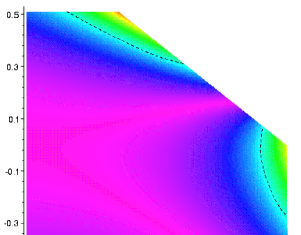
Figure 1: The fractional error in the first order approximation to angular size distance to the surface of last scatter. The dashed lines mark contours of $8\%$ error. The error is considerably less than $8\%$ across most of parameter space. The missing corner corresponds to the portion of parameter space where $\Omega_{m}=(\Omega_{0}-\Omega_{\Lambda})<0.2$.

The second major approximation was to expand the expression for $r_{sls}=R_{c}\sinh(\chi_{sls}/R_{c})$ in terms of $\Omega_{c}/\Omega_{m}$ and $\Omega_{w}/\Omega_{m}$:

$$r_{sls}=\frac{2}{H_{0}\sqrt{\Omega_{m}}}\left(1+\frac{1}{2}\frac{\Omega_{c}}{\Omega_{m}}-\frac{1}{2(1-6w)}\frac{\Omega_{w}}{\Omega_{m}}\right.$$

$$\hskip 28.90755pt-\frac{1}{8}\left(\frac{\Omega_{c}}{\Omega_{m}}\right)^{2}+\frac{3}{8(1-12w)}\left(\frac{\Omega_{w}}{\Omega_{m}}\right)^{2}$$

$$\hskip 14.45377pt\left.-\frac{3-2w}{4(1-2w)(1-6w)}\left(\frac{\Omega_{c}}{\Omega_{m}}\frac{\Omega_{w}}{\Omega_{m}}\right)+\dots\right).$$ (28)

So long as $\Omega_{m}>\Omega_{c}$ and $\Omega_{m}>\Omega_{w}$, the higher order terms can safely be neglected. Figure 1. shows the percentage error in the first order truncation of $r_{sls}$ as compared to a full numerical evaluation. The fractional error is less than $8\%$ across a wide portion of parameter space, including the interesting region around $(\Omega_{c},\Omega_{\Lambda})=(0,0.7)$.

Our final task is to show that the period of the wave responsible for the first acoustic peak is large compared to the time taken for matter and radiation to decouple. If this were not the case, the anisotropy would not be frozen in and the acoustic peak would be washed out. The conformal period of the wave is given by $T\simeq 2\pi\chi_{sh}/c_{s}$ and the conformal time interval taken to decouple is $\Delta\eta=\eta(z_{sls})-\eta(z_{sls}+\Delta z)$, where $\Delta z\approx 300$ is the redshift interval for decoupling. The ratio of $T$ to $\Delta\eta$ is given by

$$\frac{T}{\Delta\eta}\simeq 4\pi\left(\frac{z_{sls}}{\Delta z}\right)\left(1+\frac{z_{sls}}{z_{eq}}-\sqrt{\frac{z_{sls}}{z_{eq}}\left(1+\frac{z_{sls}}{z_{eq}}\right)}\right)\,.$$ (29)

For reasonable cosmological parameters, we find $T/\Delta\eta\mathrel{\hbox to0.0pt{\lower 3.0pt\hbox{$\mathchar 536\relax$}\hss}\raise 2.0pt\hbox{$\mathchar 318\relax$}}30$, which tells us that the acoustic waves are effectively snap frozen when matter and radiation decouple.

References

- (1) G. Jungman, M. Kamionkowski, A. Kosowsky and D. N. Spergel, Phys. Rev. D54, 1332 (1996).
- (2) J. R. Bond, G. Efstathiou and M. Tegmark, Mon. Not. R. Astron. Soc. 291, L33 (1997).
- (3) N.J. Cornish, D.N. Spergel & G. Starkman, Class. Quant. Grav. 15, 2657 (1998).
- (4) A good tutorial on CMBR physics and parameter fitting can be found at Wayne Hu’s homepage www.sns.ias.edu/whu/.
- (5) A.G. Doroshkevich, Ya. B. Zel’dovich & R.A. Sunyaev, Sov. Astron. 22, 523 (1978).
- (6) W. Hu and M. White, Astrophys. J. 471, 30 (1996).
- (7) A. D. Miller et al., Astrophys. J. 524 L1 (1999).
- (8) P. de Bernardis et al., Nature 404, 955 (2000).
- (9) S. Hanany et al., astro-ph/0005123, (2000).
- (10) A. E. Lange et al., astro-ph/0005004, (2000).