Event reconstruction in high resolution Compton telescopes

Abstract

The development of germanium Compton telescopes for nuclear $\gamma$-ray astrophysics ($\sim$0.2-20 MeV) requires new event reconstruction techniques to accurately determine the initial direction and energy of photon events, as well as to consistently reject background events. This paper describes techniques for event reconstruction, accounting for realistic instrument/detector performance and uncertainties. An especially important technique is Compton Kinematic Discrimination, which allows proper interaction ordering and background rejection with high probabilities. The use of these techniques are crucial for the realistic evaluation of the performance and sensitivity of any germanium Compton telescope configuration.

1 Compton telescopes for $\gamma$-ray astrophysics

Looking beyond the INTErnational Gamma-Ray Astrophysics Laboratory (INTEGRAL), the next generation soft $\gamma$-ray ($\sim$0.2-20 MeV) observatory will require high angular and spectral resolution imaging to significantly improve sensitivity to astrophysical sources of nuclear line emission. Building upon the success of COMPTEL/CGRO (Schönfelder et al. (1993)), and the high spectral resolution of the upcoming SPI/INTEGRAL (Vedrenne et al. (1998); Lichti et al. (1996)), a number of researchers (Johnson et al. (1996); Jean et al. (1996); Boggs (1998)) have discussed the merits of a high spectral/angular resolution germanium Compton telescope (GCT); the ability to achieve high sensitivity to point sources while maintaining a large field-of-view make a high resolution Compton telescope an attractive option for the next soft $\gamma$-ray observatory.

The development of Compton telescopes began in the 1970’s, with work done at the Max Planck Institut (Schönfelder et al. (1973)), University of California, Riverside (Herzo et al. (1975)), and the University of New Hampshire (Lockwood et al. (1979)), culminating in the design and flight of COMPTEL/CGRO. These historical Compton telescopes consist of two scintillation detector planes – a low atomic number ‘converter’ and a high atomic number ‘absorber.’ The model interaction of a Compton telescope is a single Compton scatter in the converter plane, followed by photoelectric absorption of the scattered photon in the absorber. By measuring the position and energy of the interactions, the event can be reconstructed to determine the initial photon direction to within an annulus on the sky.

A handful of groups are actively developing imaging germanium detectors (GeDs) partly in anticipation of a GCT (Luke et al. (1994); Kroeger et al. (1996)). The goal of these researchers is to develop large area detectors with (sub)millimeter spatial resolution, while maintaining the high spectral resolution ($E/\delta E\sim 500$ at 1 MeV) characteristic of GeDs. The use of high spectral/spatial resolution GeDs as converter and absorber planes would significantly improve the performance of a Compton telescope, but will add a number of complications to the event reconstruction. Most significantly, with the moderate atomic number $(Z=32)$ of germanium, photons will predominantly undergo multiple Compton scatters before being photoabsorbed in the instrument. Furthermore, with interaction timing capabilities of $\sim$10 ns, the interaction order will not be determined unambiguously by timing alone. Compton Kinematic Discrimination (CKD) is proposed here to overcome these complications, an extension of a method first discussed in context of liquid xenon time projection chambers (Aprile et al. (1993)). The ability of this technique to allow proper event reconstruction is investigated in detail.

Due to their relatively low efficiency (typically $\sim 1\%$), Compton telescopes rely on efficient background suppression to maintain their sensitivity. In addition to interaction ordering, techniques are presented using CKD, in combination with other tests and restrictions, to suppress the dominant background components.

The goal of this work is to outline a complete set of event reconstruction techniques for GCTs, taking into account realistic detector/instrument performance and uncertainties. Examples of the techniques are presented for a GCT configuration outlined in Appendix A; however, full analysis of this configuration will be presented in a second paper dedicated to the optimization and performance of several GCT configurations. The full analysis of a GCT configuration is complicated, requiring a detailed study of the tradeoffs between efficiency, angular and spectral resolution; therefore, this paper focuses only on the detailed discussion of the event reconstruction techniques which will be used in future work dedicated to analyzing GCT performance.

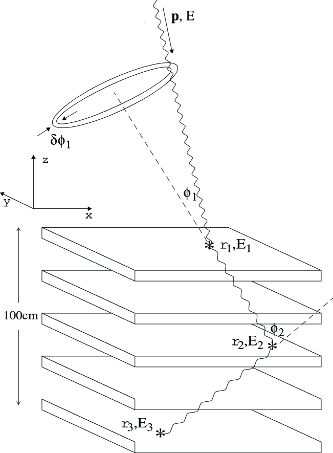
Figure 1: Example Compton telescope. If a photon undergoes one or more Compton scatters in the instrument and then is photoelectrically absorbed, then by using the positions $(\@vec{r}_{1},\ldots,\@vec{r}_{N})$ and energy deposits $(E_{1},\ldots,E_{N})$ of the interactions, the initial direction of the photon can be determined by the Compton scatter formula to within an annulus on the sky, $\phi_{1}$. The width of this annulus is determined by the uncertainties in both the interaction locations and energy deposits.

2 Principles of Compton imaging

The principle of Compton imaging of $\gamma$-ray photons is illustrated in Figure 1. (See von Ballmoos, Diehl and Schönfelder (1989) for an excellent review of historical Compton telescope configurations.) An incoming photon of energy $E$ and direction $\@vec{\hat{p}}$ undergoes a Compton scatter at an angle $\phi_{1}$ at the position $\@vec{r}_{1}$ within a detector, creating a recoil electron of energy of $E_{1}$ which is quickly absorbed and measured by the detector itself. The scattered photon then deposits the rest of its energy in the instrument in a series of one or more interactions of energies $E_{i}$ at the positions $\@vec{r}_{i}$, until eventually photoabsorbed. Here the total photon energy after each scatter $i$, normalized to the electron mass, is defined as

$$W_{i}=\frac{1}{m_{e}c^{2}}\sum_{j=i+1}^{N}E_{j}\leavevmode\nobreak\ ,$$ (1)

where $W_{0}=E/m_{e}c^{2}$, and $N$ is the total number of interactions. The initial photon direction is related to scatter direction vector $\@vec{r}_{1}^{\prime}=\@vec{r}_{2}-\@vec{r}_{1}$ ($\@vec{\hat{r}}_{1}^{\prime}$ after normalization), and the scattered photon energies $W_{i}$ by the Compton formula

$$\@vec{\hat{r}}_{1}^{\prime}\cdot\@vec{\hat{p}}=\cos{\phi_{1}}=1+\frac{1}{W_{0}}-\frac{1}{W_{1}}\leavevmode\nobreak\ .$$ (2)

Given the measured scatter direction $\@vec{\hat{r}}_{1}^{\prime}$ and the angle $\cos{\phi_{1}}$ implied from the energy depositions, the equation for $\@vec{\hat{p}}$ is not unique (if the electron recoil direction could be measured, it would solve this ambiguity); therefore, the initial direction of the photon cannot be determined directly, but it can be limited to an annulus of directions $\@vec{\hat{p}}^{\prime}$ which satisfy the equation

$$\@vec{\hat{r}}_{1}^{\prime}\cdot\@vec{\hat{p}}^{\prime}=\cos{\phi_{1}}\leavevmode\nobreak\ .$$ (3)

There are two uncertainties in determining the event annulus: the uncertainty in $\phi_{1}$ due to the finite energy resolution of the detectors, here labelled $\delta\phi_{1,E}$, and the uncertainty in $\@vec{r}_{1}^{\prime}$ determined by the spatial resolution of the detectors. Both of these uncertainties add to determine the uncertainty (effective width) of the event annulus $\delta\phi_{1}$. From Equation 2, the derivation of $\delta\phi_{1,E}$ is straightforward and yields

$$\delta\phi_{i,E}=\frac{1}{\sin{\phi_{i}}}[(\frac{\delta W_{i-1}^{2}}{W_{i-1}^{4}})+\delta W_{i}^{2}((\frac{1}{W_{i}^{2}}-\frac{1}{W_{i-1}^{2}})^{2}-\frac{1}{W_{i-1}^{4}})]^{1/2}\leavevmode\nobreak\ ,$$ (4)

where,

$$\delta W_{i}=\frac{1}{m_{e}c^{2}}[\sum_{j=i+1}^{N}\delta E_{j}^{2}]^{1/2}\leavevmode\nobreak\ .$$ (5)

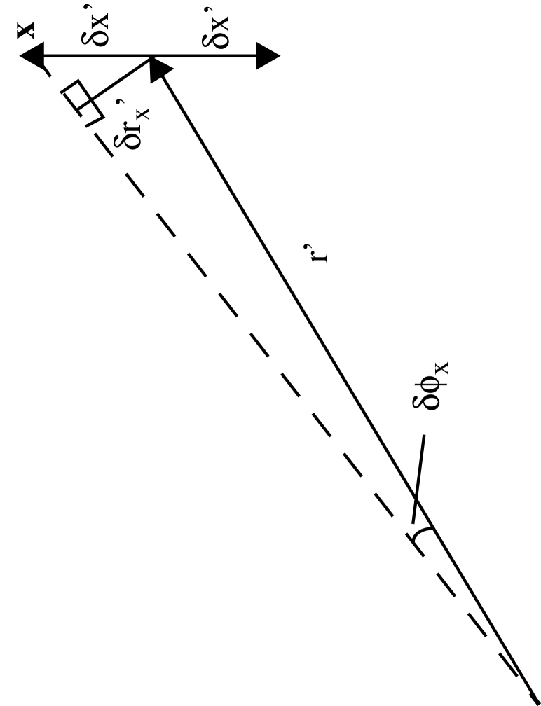
Figure 2: Illustration of how uncertainties in the scattered photon direction $\@vec{r}^{\prime}$ can be translated into effective uncertainties in the scattering angle $\phi$.

In order to simplify the analysis, it is convenient to transform the uncertainty $\delta\@vec{r}_{1}^{\prime}$ into an effective uncertainty in $\phi_{1}$, defined as $\delta\phi_{1,r}$, such that

$$\delta\phi_{1}=\sqrt{\delta\phi_{1,E}^{2}+\delta\phi_{1,r}^{2}}\leavevmode\nobreak\ .$$ (6)

The angular resolution $\delta\phi_{i,r}$ is the effective ‘wiggle’ of $\@vec{\hat{r}}_{i}^{\prime}$ around its measured direction due to the uncertainties in the spatial measurements. The spatial uncertainties are defined as $\delta x^{\prime}_{i}=\sqrt{\delta x_{i}^{2}+\delta x_{i+1}^{2}}$, $\delta y^{\prime}_{i}=\sqrt{\delta y_{i}^{2}+\delta y_{i+1}^{2}}$, $\delta z^{\prime}_{i}=\sqrt{\delta z_{i}^{2}+\delta z_{i+1}^{2}}$. It is simplest to analyze the situation for each axis separately as shown in Figure 2. The uncertainty in the direction of $\@vec{\hat{r}}_{i}^{\prime}$ due to the uncertainty $\delta x^{\prime}_{i}$ is given by

$$\delta\phi_{i,x}\simeq\tan(\delta\phi_{i,x})=(\frac{\delta x^{\prime}_{i}}{r_{i}^{\prime}})\sqrt{1-(\@vec{\hat{r}}_{i}^{\prime}\cdot\@vec{\hat{x}})^{2}}\leavevmode\nobreak\ .$$ (7)

Likewise for the other axis,

$$\delta\phi_{i,y}\simeq(\frac{\delta y^{\prime}_{i}}{r_{i}^{\prime}})\sqrt{1-(\@vec{\hat{r}}_{i}^{\prime}\cdot\@vec{\hat{y}})^{2}}\leavevmode\nobreak\ ,$$

$$\delta\phi_{i,z}\simeq(\frac{\delta z^{\prime}_{i}}{r_{i}^{\prime}})\sqrt{1-(\@vec{\hat{r}}_{i}^{\prime}\cdot\@vec{\hat{z}})^{2}}\leavevmode\nobreak\ ,$$

which combine to yield the total uncertainty $\delta\phi_{i,r}$ given by

$$\delta\phi_{i,r}=\sqrt{\delta\phi_{i,x}^{2}+\delta\phi_{i,y}^{2}+\delta\phi_{i,z}^{2}}\leavevmode\nobreak\ .$$ (8)

For detectors with a given energy resolution, in order to optimize the performance of a Compton telescope one would require that $\delta\phi_{i,r}\leq\delta\phi_{i,E}$ in the energy range of interest. To first order, this implies that the spatial resolution in relation to the scale size of the instrument must be comparable to or less than the energy resolution, i.e. $\delta r_{1}^{\prime}/r_{1}^{\prime}\leq\delta E_{1}^{\prime}/E_{1}^{\prime}$.

3 Complications of germanium Compton telescopes

Finite detector thresholds, energy resolutions, and spatial resolutions produce systematic biases in the imaging capabilities of Compton telescopes. These limitations have been discussed in detail elsewhere in context of two-layer, low-Z converter and high-Z absorber, scintillation detector designs (von Ballmoos et al. (1989)), and the conclusions can be directly applied to GCTs. However, GCT designs will introduce additional complications which significantly alter the event reconstruction techniques. Historical Compton telescope configurations make two assumptions about the events which do not generally hold in GCTs: (i) the events are a single Compton scatter in the converter, followed by photoelectric absorption in the absorber, and (ii) the time-of-flight (TOF) between the photon interactions is measured to determine their order.

The distributions of number and type of interaction sites in a GCT for normally incident, fully-absorbed photons ranging from 0.2-10 MeV are shown in Figure 3, for the instrument configuration discussed in Appendix A. Here we distinguish three event types: a single photoelectric absorption, one or more Compton scatters followed by a single photoabsorption, and one or more pair productions. Compton scatters followed by pair production could potentially be reconstructed; however, here we include these events with other pair productions. These distributions account for the finite spatial resolution of the detectors, so that interactions occurring too closely together are not resolved. From these distributions it is clear that events with $\sim$8 or more interaction sites can be immediately rejected as probable pair production events, with little effect on the Compton photopeak efficiency. For incident photon energies above 0.5 MeV, 3-7 interaction site Compton scatter events dominate the photopeak.

To accurately reconstruct a Compton scatter event, the first and second interaction sites must be spatially resolved, and their order correctly determined. The need to determine the proper ordering of three or more (3+) interaction sites is complicated by the timing capabilities of GeDs. In the scintillation detectors of COMPTEL/CGRO the interaction timing can be performed to $\sim$0.25 ns (Schönfelder et al. (1993)), which is adequate to determine the TOF between two interactions in the separate detector planes. With the slower rise time of GeDs one can reasonably expect event timing to $\sim$10 ns, which is inadequate for TOF measurement in reasonably-sized instruments. While Pulse Shape Discrimination methods have been proposed to push the interaction timing in GeDs to $\sim$1 ns (Boggs (1998)), even this timing would be unreliable for determining TOF among three or more interaction sites. A method of reliably determining the photon interaction order without timing information must be developed.

Figure 3: Statistical distributions of the number of interaction sites for fully-absorbed photons for the instrument configuration presented in Appendix A. These distributions take into account the finite spatial distribution of the detectors, combining interactions that cannot be spatially resolved. Events are divided into photoelectric absorptions (solid white), pair productions (solid black), and the desired Compton scatter(s) followed by a single photoabsorption (striped). Events with 12 or more sites were combined in a single bin.

4 Multiple Compton scatter events: Compton kinematic discrimination

One method has been suggested to overcome these complications in the context of liquid xenon time projection chambers (Aprile et al. (1993)). Here, this method is formalized as Compton Kinematic Discrimination (CKD) and examined in more detail. This technique allows the order of the photon interactions to be determined with high probability, as well as providing the basis of a powerful tool for background suppression in GCTs.

CKD takes advantage of redundant measurement information in an event to determine the most likely interaction sequence. A photon of initial energy $E$ (using the notation in Section 2) interacts in the instrument at $N$ sites, depositing an energy of $E_{i}$ at each location $\@vec{r}_{i}$. It is assumed that the interactions $1,\ldots,N-1$ are Compton scatters, and interaction $N$ is the final photoabsorption. Given the correct ordering of the interactions, there are two independent ways of measuring $N-2$ of the scattering angles, $\cos{\phi_{2}},\ldots,\cos{\phi_{N-1}}$.

Geometrical measurement of $\cos{\phi_{i}}$. From simple vector analysis, given the correct ordering of the interaction sites one can derive the scatter angles

$$\cos{\phi_{i}}=\@vec{\hat{r}}_{i}^{\prime}\cdot\@vec{\hat{r}}_{i-1}^{\prime},i=2,\ldots,N-1\leavevmode\nobreak\ ,$$ (9)

where the uncertainties in the scattering angles, $\delta\cos{\phi_{i}}$, can be estimated from the spatial uncertainty in the scattering angles (Equation 8), yielding

$$\delta(\cos{\phi_{i}})=\delta\phi_{i,r}\sin{\phi_{i}}\leavevmode\nobreak\ .$$ (10)

Compton kinematics measurement of $\cos{\phi_{i}^{\prime}}$. Given the correct ordering, the measured values of $W_{i}$ can be derived, which were defined earlier as the energy of the photon after each scattering $i$, in units of $m_{e}c^{2}$. The Compton scatter formula (Equation 2) gives:

$$\cos{\phi_{i}^{\prime}}=1+\frac{1}{W_{i-1}}-\frac{1}{W_{i}},i=1,\ldots,N-1\leavevmode\nobreak\ ,$$ (11)

$$\delta(\cos{\phi_{i}^{\prime}})=[(\frac{\delta W_{i-1}^{2}}{W_{i-1}^{4}})+\delta W_{i}^{2}((\frac{1}{W_{i}^{2}}-\frac{1}{W_{i-1}^{2}})^{2}-\frac{1}{W_{i-1}^{4}})]^{1/2}\leavevmode\nobreak\ .$$ (12)

Given the $N-2$ independent measurements of $\cos{\phi_{2}},\ldots,\cos{\phi_{N-1}}$, a trial ordering of the interaction sites can be tested for consistency. If the assumed ordering is incorrect $\cos{\phi_{i}}$ will not equal $\cos{\phi_{i}^{\prime}}$ in general. Every possible permutation of orderings can be tested to determine the one most consistent with $\cos{\phi_{i}}=\cos{\phi_{i}^{\prime}}$. Given a trial ordering, the two angle cosines for sites $i=2,\ldots,N-2$ are relabelled for convenience $\eta_{i}=\cos{\phi_{i}}$, $\eta_{i}^{\prime}=\cos{\phi_{i}^{\prime}}$.

As a first test, trial orderings that produce values of $\mid\eta_{i}^{\prime}\mid\geq 1$ are ruled out, since $\cos{\phi_{i}^{\prime}}<1$ for any scattering angle $\phi_{i}^{\prime}$. This condition will eliminate many orderings which cannot physically be due to multiple Compton scatters followed by photoabsorption. Next a least-squares statistic measuring the agreement between the redundant scatter angle measurements is defined:

$$\chi^{2}=\frac{1}{N-2}\sum_{i=2}^{N-1}\frac{(\eta_{i}-\eta_{i}^{\prime})^{2}}{(\delta\eta_{i}^{2}+\delta\eta_{i}^{\prime 2})}\leavevmode\nobreak\ .$$ (13)

In general, $\chi^{2}$ will be minimized when the interactions are properly ordered (i.e. the order in which they occurred). Therefore, all possible permutations can be tested for their value of $\chi^{2}$, and the ordering corresponding to the minimum value, $\chi^{2}_{min}$, is taken as the most likely ordering.

This consistency statistic also provides a powerful tool for rejecting background events. If the event is truly a multiple Compton scatter event followed by a photoabsorption then $\chi^{2}_{min}\sim 1$. By setting a maximum acceptable level for $\chi^{2}_{min}$, events that do not fit this scenario can be rejected. Such events include partially-deposited photons which scatter out of the instrument (Compton continuum), photon interactions with spatially unresolved interaction sites, events with interactions below the detector threshold, pair-production events, and similarly $\beta^{+}$ decays. These events frequently have $\chi^{2}_{min}\gg 1$, allowing a strong rejection statistic that is not very sensitive on the level set on $\chi^{2}_{min}$. Here, $\chi^{2}_{min}$ has been treated as a normal least-squares statistic with $N-2$ degrees of freedom, and events are rejected which have probabilities of $\chi^{2}_{min}<5\%$. Variations in the level between $1\%$ and $10\%$ do not strongly affect CKD rejection capabilities. For example, varying this level from $5\%$ to $1\%$ shifted the CKD efficiency curves in Figure 4 by 1-2%.

Figure 4: Photopeak distributions for 3+ site events. The fraction of events with the first and second interaction sites spatially resolved are presented ($\diamond$), along with the fraction of events which have been properly ordered (hence imaged) using CKD ($\triangle$). The fraction of events rejected by the CKD statistic ($\Box$) as well as the fraction incorrectly imaged ($\times$) are also shown.

The fraction of 3+ site photopeak events which have the first and second interaction sites spatially resolved – and hence could be imaged to the proper direction – is shown in Figure 4 as a function of energy, for the instrument model discussed in Appendix A. Roughly $90\%$ of all events from 0.2-20 MeV have their first and second sites spatially resolved from each other. (Some of these events do not have their second, third, etc., interactions spatially resolved from each other, and will be rejected by the limits on $\chi^{2}_{min}$.) This figure also shows the fraction of the photopeak events which CKD properly orders (correctly reconstructed), as well as the fractions improperly ordered (hence incorrectly imaged to off-source background), and the fraction completely rejected. For energies below $\sim$10 MeV, CKD allows proper reconstruction (hence imaging) of $\sim 60-70\%$ of the photopeak events, while rejecting $10-20\%$. The remaining $10-20\%$ are incorrectly imaged into the off-source background. For comparison, if the order of the interaction sites were randomly chosen $<15\%$ would be correctly imaged, while the remaining $>85\%$ would be incorrectly imaged into the background.

5 Single Compton scatter events: single scatter discrimination

CKD will only work for $N>2$ since there are no independent scattering angle measurements for a single Compton scatter followed by a photoabsorption. It turns out that the ordering of two-site photopeak events can still be determined with a high probability; however, the ability to reject background events is lost. As is discussed further in Section 6, the loss of background rejection, coupled with low peak-to-Compton ratios, and a larger fraction of backscatter events mean that the inclusion of two-site events will likely hurt the sensitivity of a GCT; however, discussion of event ordering is still included for completeness.

Given a two-site event, the first test one can perform is to determine whether both possible orderings of the interaction sites are energetically compatible with a single Compton scatter, i.e. are compatible with the requirement that $\cos{\phi_{1}}<1$ (Equation 2). In Figure 5, the fraction of spatially-resolved, photopeak events with unique orderings are plotted versus energy. Also plotted are the fraction with ambiguous orderings. At energies below $\sim$0.4 MeV the majority of resolved photopeak events have a unique ordering, while at higher energies most events are ambiguous.

As an empirical test of the ambiguous events, the relative magnitude of the energy lost in the initial scatter $(E_{1})$ compared to the photoabsorption $(E_{2})$ can be compared. The fraction of resolved two-site photopeak events which have ambiguous orderings with $E_{1}>E_{2}$ is plotted in Figure 5. At higher energies, nearly all of the resolved photopeak events with ambiguous interaction orders have $E_{1}>E_{2}$, which can be used to determine the most likely interaction order. This empirical result can be easily understood, in hindsight, by the fact that photons which deposit most of their energy in the initial Compton scatter are much more likely to be photoabsorbed in the second interaction.

Figure 5: Empirical distributions for fully-resolved, two-site photopeak events. The fraction of events with only one physically possible ordering ($\Box$), as well as events with both orderings physically possible ($\triangle$) are shown. Also shown are the events with both orderings possible, but with the larger energy deposit in the initial scatter rather than the photoabsorption, $E_{1}>E_{2}$ ($\diamond$).

Therefore, a simple Single Scatter Discrimination (SSD) technique to determine the most likely interaction ordering of two-site events follows. First one determines whether a physically unique ordering exists; if not, the larger energy deposit is assumed to be the initial Compton scatter. Only at the lowest energies are two-site events possible in which neither ordering is acceptable (unresolved events, Compton continuum), and some background rejection is possible.

The fraction of two-site photopeak events which are spatially resolved is shown in Figure 6 as a function of energy, for the instrument model in Appendix A. Roughly $80\%$ of all events from 0.2-20 MeV are resolved. This number is about $10\%$ lower than the 3+ site events, due to the smaller path lengths of the lower energy scattered photons in two-site photopeak events. Also shown in Figure 6 is the fraction of events which SSD has properly reconstructed. SSD allows proper reconstruction (hence imaging) of $\sim 60-80\%$ of the photopeak events, while improperly imaging the remaining $\sim 20-40\%$ into the off-source background. Only a relatively small number of low energy events can be rejected outright. SSD is least effective around 0.5 MeV, where the unique/ambiguous ordering signatures are not as clear. For comparison, if the order of the interaction sites were randomly chosen $\sim 40\%$ would be properly imaged, while the remaining $\sim 60\%$ would be improperly imaged into the background.

Figure 6: Photopeak distributions for two-site events. The fraction of events with the first/second interaction sites spatially resolved are presented ($\diamond$), along with the fraction of events which have been properly ordered (hence imaged) using SSD ($\triangle$). The fraction of events rejected due to no physically possible orderings ($\Box$), as well as the fraction incorrectly imaged ($\times$) are also shown.

6 Full reconstruction with background rejection

Given these two methods of determining the photon interaction order in GCTs, CKD and SSD, a full event reconstruction technique incorporating other background rejection techniques can be developed. The high spectral and spatial resolution of a GCT make several powerful background rejection techniques possible. The predominance of multiple scattering events, while initially a complication, dramatically helps in the overall background rejection.

The dominant sources of background in GCTs are expected to be diffuse cosmic $\gamma$-ray emission, induced satellite $\gamma$-ray emission, and induced $\beta^{+}$, $\beta^{-}$ radioactivities in the GeDs themselves (Jean et al. (1996); Graham et al. (1997); Gehrels (1985); Dean et al. (1991); Naya et al. (1996)). Source/background photons which scatter out of the instrument before depositing all of their energy, and hence are improperly imaged, must also be included in these calculations.

Restrictions on the acceptable events can have a dramatic effect on sensitivity of a GCT. Specifically, several factors can affect the angular resolution of the instrument as well as the background rates – such as the inclusion of backscatter events, limits on the accepted scatter angles, and the minimum acceptable lever arm – and must be included in any discussion of full reconstruction and background rejection.

6.1 Shield veto

Placing an active shield below the bottom GCT detector plane could be useful for rejecting background photons from below the instrument (induced satellite $\gamma$-ray emission), as well as helping to reject Compton continuum and $\beta-$decay events in the instrument. However, many of these events can be distinguished and rejected using CKD and other tests/restrictions outlined below; therefore, the usefulness of including a shield in the GCT design must be studied in detail for a given telescope configuration.

6.2 Restrictions on number of interaction sites: pair production/$\beta^{+}$ decays

While it is obvious that any single-site interactions should be rejected in a Compton telescope, events with $\sim$8 or more interaction sites should also be rejected since these are very likely due to pair production events, as is evident from Figure 3, or similarly $\beta^{+}$ decays. (See Section 6.8)

6.3 CKD $\chi^{2}_{min}$ test: Compton continuum, unresolved interactions, etc.

Using the tests outlined in Sections 4 and 5, the most likely ordering of the interaction sites can be determined, and for 3+ site events many of the unresolved and Compton continuum events, as well as pair production and $\beta-$decays, rejected.

Shown in Figure 7 is the peak-to-Compton ratio for 3+ site events, here defined as the ratio of the properly imaged photopeak events to the corresponding integrated Compton continuum (photons which scatter out of the instrument before depositing all of their energy). This standard measure for $\gamma$-ray spectroscopy instruments has an altered meaning here, since the Compton continuum events will be incorrectly imaged, and thus will appear as off-source background. The peak-to-Compton ratio is shown both before and after rejection of the continuum events with the CKD statistic. CKD rejection of the Compton continuum events increases the peak-to-Compton ratio by factors of 3-6, an important improvement for low background instruments. By rejection of events appearing to originate from below the instrument (Section 6.4), as well as backscattered interactions (Section 6.5), this ratio can be increased by further factors of 2-4.

Also shown in Figure 7 is the photopeak-to-Compton ratio for two-site events using SSD, which is significantly lower than the corresponding ratio for 3+ site events. In fact, this ratio drops significantly below unity, which means that more background than signal is being created in the instrument for two-site events. This result questions whether two-site events should be included in actual observational analysis given the accompanying increase in unrejectable background. This conclusion is further supported by the fact that the majority of two-site events are backscatters (Section 6.5), which will significantly degrade the angular resolution. Even though inclusion of two-site events is unlikely to improve the overall sensitivity for GCTs, detailed background analysis for specific instrument configurations is required to determine the overall effects.

Figure 7: Peak-to-Compton ratios. Shown are the ratios of correctly ordered (imaged) photopeak events to integrated Compton continuum events for: 3+ sites before CKD rejection ($\diamond$), 3+ sites after CKD rejection ($\triangle$), and two-site events ($\Box$).

6.4 Effective TOF

Once the most likely order of interactions and the initial scatter angle are determined, it is possible to determine whether the incident photon scattered upwards or downwards in the instrument, as well as whether the initial scatter was forward or backwards. Thus, events which appear to be photons originating from below the instrument can be rejected, which include the induced satellite $\gamma$-ray emission, many Compton continuum events which were not rejected by CKD, photons which scatter in the passive satellite material before interacting in the detectors, and many of the pair production and $\beta-$decay events. The simulation results for the configuration in Appendix A show that $\sim 95\%$ of photons originating from below the instrument are rejected.

6.5 Backscatters

Once the most likely ordering of interaction sites has been determined, this information can also be used to accept/reject backscattered source photons. The fraction of photopeak events which backscatter during the initial interaction is not strongly energy dependent, $\sim 60-70\%$ for two site events, and $\sim 30\%$ for 3+ site events. These events can significantly increase the effective area at lower energies, where two-site events are most common, at the expense of degrading the angular resolution due to larger uncertainties in $\delta\phi_{1,E}$ for backscatters events (Equation 4). It is unlikely that the overall sensitivity will improve by including backscattered events given the increased background rates and degraded angular resolution; however, the effects on sensitivity will depend on the exact instrument configuration and observational goals.

6.6 ‘Standard $\phi$ restriction’

Restrictions can also be set on the scattering angles accepted for forward-scattering photons entering the front of the instrument. These limits can be used to restrict the instrument FOV to improve imaging capabilities and background, such as the ‘standard $\phi$ restriction’ (Schönfelder et al. (1982)). These restricitions will have to be reanalyzed in detail for specific GCT configurations.

6.7 Nonlocalized $\beta^{-}$ decays

In a nonlocalized $\beta^{-}$ decay, the daughter nuclide is produced in an excited state which quickly decays on timescales relative to the detector collection time, emitting a photon with energy characteristic to the daughter nuclide. Therefore, the event consists of the intial $\beta^{-}$ decay site, plus the interaction sites of the emitted photon. Such an event can be rejected if the characteristic photon energy can be detected in any combination of the interaction site energies. The seven dominant $\beta^{-}$ isotopes and characteristic photon energies for natural Ge are given in Table 1 (Naya et al. (1996); Gehrels (1985)). In general, if the coincident $\gamma$-ray is fully deposited, then the event will have $\chi^{2}_{min}\sim 1$, with the $\beta^{-}$ electron interaction ordered as the initial ‘scatter’ site. In these cases, $W_{1}$ will have the characteristic photon energy specific to that decay. The rejection of all events with $W_{1}$ equal to one of the characteristic energies in Table 1 can dramatically decrease the $\beta^{-}$ decay background, with only a small effect, typically $\leq 3\%$ drop in photopeak efficiencies for true photon events. More $\beta^{-}$ decays can be rejected if every possible combination of interaction sites is tested for the decay photon energies, at the expense, however, of more rejection of photopeak events, typically $\sim 15-20\%$. If the coincident $\gamma$-ray is only partially deposited, the event will likely be rejected by the limits set on $\chi^{2}_{min}$.

Table 1: Characteristic photon energies for the strongest nonlocalized $\beta^{-}$ decays in natural Ge.

$$\begin{array}[]{p{0.5\linewidth}l}\hline\cr\vskip 3.0pt plus 1.0pt minus 1.0pt\cr daughter&photon\leavevmode\nobreak\ energy\\ \vskip 3.0pt plus 1.0pt minus 1.0pt\cr\hline\cr\vskip 3.0pt plus 1.0pt minus 1.0pt\cr${}^{75}Ge$&0.265\leavevmode\nobreak\ MeV\\ ${}^{73}Ga$&0.297\leavevmode\nobreak\ MeV\\ ${}^{72}Ga$&0.834\leavevmode\nobreak\ MeV\\ ${}^{71}Zn$&0.512\leavevmode\nobreak\ MeV\\ ${}^{76}As$&0.559\leavevmode\nobreak\ MeV\\ ${}^{28}Al$&1.779\leavevmode\nobreak\ MeV\\ ${}^{77}Ge$&0.216\leavevmode\nobreak\ MeV\\ \vskip 3.0pt plus 1.0pt minus 1.0pt\cr\hline\cr\end{array}$$

$\beta^{-}$ decay background events were simulated for the instrument discussed in Appendix A. The results of these background calculations will be presented in a separate paper, but here we make preliminary use of these simulations to demonstrate the background rejection capabilities. After initial rejection of two site ($34.4\%$) and 8+ site ($2.9\%$) events, $62.7\%$ of the nonlocalized $\beta^{-}$ events remain. Applying the CKD test, requiring a $5\%$ probability of $\chi^{2}_{min}$, brings the remaining number of decays down to 17.9%. After screening the interactions for characteristic $\beta^{-}$ decay energies, this number is reduced to $9.3\%(15.1\%)$. Finally, after rejecting events which appear to originate from below the instrument, or which appear to be backscatter events, the final number of unrejected $\beta^{-}$ decays comes to $4.2\%(6.8\%)$, a factor of 20 (15) reduction in this background component. (First numbers give results when all combinations of interaction sites are searched for $\beta^{-}$ decay energies, while the numbers in parenthesis are results when only $W_{1}$ is tested. Typical errors $\sim 0.2\%$.)

6.8 Positron signatures

A further test for rejecting the pair production/$\beta^{+}$ background events that survive the other tests/restrictions outlined above is to search for positron annihilation signatures in the interaction energies. By analyzing all combinations of the interaction sites to see if the energies sum to $m_{e}c^{2}=0.511\leavevmode\nobreak\ MeV$, events with a positron annihilation signature can be rejected. This test typically reduces the non-pair production photopeak events by $\leq 2\%$.

$\beta^{+}$ background events were simulated for the instrument discussed in Appendix A. After initial rejection of two site events ($23.0\%$) and 8+ site events ($3.0\%$), $74.0\%$ of the events remain. After the CKD test, $16.7\%$ remain. After screening the interactions for 0.511 MeV positron annihilation signatures, the number is reduced to $5.2\%$. Finally, after rejecting events which appear to originate from below the instrument, or which appear to be backscatter events, the final number of unrejected $\beta^{+}$ events is $1.9\%$, a factor of 50 reduction in this background component. Similar reductions occur when these tests are applied to pair production events. (Typical errors $\sim 0.1\%$.)

6.9 Minimum lever arm

In general, a minimum acceptable distance between the first and second interaction sites – the lever arm – must be set. Figure 8 shows the fraction of 0.5 and 2.0 MeV photopeak events with lever arms above a given level, for the instrument configuration in Appendix A. Similar to the case of backscattered events, a smaller minimum lever arm means a higher effective area at the expense of poorer angular resolution. The exact lever arm chosen will depend on the instrument configuration and observational goals.

Figure 8: The fraction of 0.5 and 2.0 MeV photopeak events with lever arms (separations between the first and second interaction sites) greater than the specified values for the model in Appendix A. Shown for comparison are several characteristic distances of this model.

Table 2: Percentage of events remaining after subsequent application of rejection techniques.

$$\begin{array}[]{p{0.2\linewidth}|*{6}{lccccc}}\hline\cr\vskip 3.0pt plus 1.0pt minus 1.0pt\cr rejection&0.5MeV&2.0MeV&$$\beta^{-}$$decays&$$\beta^{+}$$decays&spacecraft\\ technique&photopeak&photopeak&&&\\ \vskip 3.0pt plus 1.0pt minus 1.0pt\cr\hline\cr\vskip 3.0pt plus 1.0pt minus 1.0pt\cr 2 site events&65.0\%&82.0\%&65.6\%&77.0\%&61.6\%\\ 8+ site events&64.9\%&80.9\%&62.7\%&74.0\%&60.8\%\\ CKD&51.2\%&61.4\%&17.9\%&16.7\%&35.2\%\\ $\beta$ signatures&48.4\%&58.0\%&15.1\%&5.2\%&32.2\%\\ backscatter/TOF&35.5\%&38.5\%&6.8\%&1.9\%&12.2\%\\ min lever arm (10 cm)&15.0\%&16.7\%&2.0\%&1.2\%&2.6\%\\ \vskip 3.0pt plus 1.0pt minus 1.0pt\cr\hline\cr\end{array}$$

7 Conclusions

Event reconstruction in future high resolution Compton telescopes will present a number of complications compared to historical configurations. The initial complication of multiple-scattering of photons in GCTs, however, turns out to be an advantage: the application of CKD to 3+ site events, combined with the high spectral and spatial resolution of GeDs, allows extremely efficient background suppression, crucial for Compton telescope performance. This paper has outlined a set of tests and restrictions, accounting for realistic instrument/detector performance, to reconstruct photopeak events in GCTs while rejecting a large fraction of the background events. Table 2 presents the fraction of events, photon and background, that remain after each rejection technique is subsequently applied. (The numbers in Table 2 assume only $W_{1}$ is tested for $\beta^{-}$ decay energies.) Development of these event reconstruction techniques allows realistic evaluation of the performace and sensitivity of GCT designs. Our next goal is to simulate the efficiency, resolution, background and sensitivity of several Compton telescope configurations, utilizing the event reconstruction techniques developed here to realistically determine the performace of these instruments. CKD rejection has been shown to be the most efficient background rejection technique; however, the addition of effective TOF, backscatter, nonlocalized $\beta^{-}$ decay, and positron signature tests dramatically improve background rejection capabilities. We anticipate that use of these techniques will achieve overall sensitivity improvements in GCTs by factors of $\sim 5-10$.

S. E. Boggs would like to thank the Millikan Postdoctoral Fellowship Program, CIT Deparment of Physics, for support.

Appendix A Example GCT configuration

While it is not the intention of this paper to fully characterize the performance of a specific GCT, it is useful to have a telescope model for which the results of the event reconstruction can be presented. The telescope configuration modeled in this study is presented in Figure 1. The instrument consists of five planar arrays of 15 mm thick germanium, each of area $100\leavevmode\nobreak\ cm\times 100\leavevmode\nobreak\ cm$. In reality each array would consist of separate smaller detectors $(\sim 5\leavevmode\nobreak\ cm\times 5\leavevmode\nobreak\ cm)$ tiled to form the entire plane; however, the simulation performed here modeled each plane as a solid detector for simplicity. The five planar arrays are spaced 20 cm apart.

This configuration differs from historical Compton telescope configurations which generally consist of two detector planes separated by 100-150 cm. This separation distance is determined by the spatial resolution in z and the desired angular resolution. As will be discussed in a second paper, the configuration modeled here significantly improves the effective area of the telescope by letting each plane act as converter, and permitting a much wider range of scatter angles to produce good events. Allowing large-angle scatters also significantly increases the instrument FOV, and limits the effects of point spread function smearing for sources at large off-axis angles. The potential drawbacks of this configuration are increased background and degraded angular resolution.

The instrument was simulated using CERN’s GEANT Monte Carlo code. The Monte Carlo simulation produces a file of interaction locations and energy depositions for each photon/$\beta-$decay event. Before performing event reconstruction on the interactions, the simulated events are modified to reflect realistic measurement uncertainties of an instrument: for each interaction, a random Gaussian-distributed uncertainty is added to the energy and position of each interaction. All interaction locations which lie within twice the instrumental spatial resolution of each other are combined into a single interaction site, to accurately reflect the resolving power of the detectors. Finally, interaction sites with energy deposits below the assumed detector threshold of 10 keV are ignored.

Figure 9: Assumed resolutions for the GCT model. (Left) The total energy resolution (solid line) is determined by the electronic noise (dotted line) and the intrinsic resolution (dashed line) added in quadrature. (Right) The total x-, y- (solid line) and z- (dot-dashed line) spatial resolution are determined by the segmentation/signal processing limits (dotted line), and the recoil electron range (dashed line) added in quadrature. (See text for details.)

Two components are assumed to add in quadrature to determine the energy resolution: (i) a constant electronic noise, $W_{e}=1.0\leavevmode\nobreak\ keV\leavevmode\nobreak\ FWHM$, and (ii) the intrinsic resolution $W_{i}$ determined by the germanium Fano factor, $F=0.13$, and average free electron-hole pair energy, $\varepsilon=2.98\leavevmode\nobreak\ eV$, giving $W_{i}=2.35\sqrt{F\varepsilon E}\leavevmode\nobreak\ FWHM$. This corresponds to a resolution $\sim 1.8\leavevmode\nobreak\ keV\leavevmode\nobreak\ FWHM$ at 1 MeV, which is optimistic but not unrealistic. It is assumed that charge trapping and ballistic deficit do not significantly alter this energy resolution. The two components as well as the total energy resolution are shown in Figure A1.

It is assumed that two components add in quadrature to determine the $1-D$ spatial resolutions, $\delta x,\delta y,\delta z$, of the detectors: (i) the range of the recoil electrons in the detector, and (ii) the positioning limits of the detector due to physical segmentation and/or signal analysis. Calculated electron ranges in germanium for different energies (Mukoyama (1976)) are used here as the 1-D FWHM positional uncertainties, $\delta x_{e},\delta y_{e},\delta z_{e}$. Methods to determine the event position by physically segmenting the GeD contacts into cross strips or pixels (Luke et al. (1994); Kroeger et al. (1996)), as well as using advanced signal processing to interpolate to even better positions (Boggs (1998); Luke et al. (1994)), are currently active fields of research – so this component of the spatial resolution remains speculative for now. Here it is assumed that signal processing will allow positional resolutions of $\sim 0.5\leavevmode\nobreak\ mm\leavevmode\nobreak\ FWHM$ at 100 keV, and that the discrimination capabilities go as the signal-to-noise ratio of the induced detector signal to electronic noise, i.e. as the inverse power of the interaction energy. It is also assumed that there is $\sim 1\leavevmode\nobreak\ mm$ physical segmentation of the detector contacts in x, y, so that this component never exceeds this value. The z uncertainty, however, is not constrained by any such segmentation at the lowest energies. Therefore, the signal processing uncertainty is given by $\delta x_{s},\delta y_{s},\delta z_{s}\sim 0.50(E/100keV)^{-1}\leavevmode\nobreak\ mm\leavevmode\nobreak\ FWHM$, maximizing at 1 mm in x, y below 50 keV, and approaching, but never maximizing at 15 mm in z at low energies. The two components as well as the total spatial resolution are shown in Figure A1.

References

- Aprile et al. (1993) Aprile E., Bolotnikov A., Chen D., Mukherjee R., 1993, Nucl. Inst. & Methods A 327, 216
- Boggs (1998) Boggs S. E., 1998, Ph. D. Dissertation, University of California, Berkeley
- Dean et al. (1991) Dean A. J., Lei F., Knight P. J., 1991, Space Sci. Rev. 57, 109
- Gehrels (1985) Gehrels N., 1985, Nucl. Inst. & Methods A 239, 324
- Graham et al. (1997) Graham B. L., Phlips B. F., Kurfess J. D., Kroeger R. A., 1997, IEEE Nucl. Sci. Symp. N23-3
- Herzo et al. (1975) Herzo D., et al. 1975, Nucl. Inst. & Meth. 123, 583
- Jean et al. (1996) Jean P., Naya J. E., Olive J. F., von Ballmoos P., 1996, A&ASS 120, 673
- Johnson et al. (1996) Johnson W. N., et al., 1996, SPIE
- Kroeger et al. (1996) Kroeger R. A., et al., 1996, IEEE
- Lichti et al. (1996) Lichti G. G., et al., 1996, SPIE 2806, 217
- Luke et al. (1994) Luke P. N., et al, 1994, IEEE
- Lockwood et al. (1979) Lockwood J. A., Hsieh L., Friling L., Chen C. & Swartz D., 1979, JGR 84, 1402
- Mukoyama (1976) Mukoyama, T., 1976, Nucl. Inst. & Meth. 134, 125
- Naya et al. (1996) Naya J. E., et al., 1996, Nucl. Inst. & Meth. A 368, 832
- Schönfelder et al. (1973) Schönfelder V., Hirner A., & Schneider K., 1973, Nucl. Inst. & Meth. 107, 385
- Schönfelder et al. (1982) Schönfelder V., Graser U., & Diehl R., 1982, A&A 110, 138
- Schönfelder et al. (1993) Schönfelder V., et al. 1993, ApS 86, 657
- Vedrenne et al. (1998) Vedrenne G., Schönfelder V., et al., 1998, Proc. 3rd INTEGRAL Workshop, Taormina
- von Ballmoos et al. (1989) von Ballmoos P., Diehl R., & Schönfelder V., 1989, A&A 221, 396