Magnetic fields around black holes

Abstract

Mutual interaction between electromagnetic and gravitational fields can be treated in the framework of the general theory of relativity. This poses a difficult problem but different approximations can be introduced in order to grasp interesting effects and to describe mechanisms which govern astronomical objects.

The electromagnetic field near a rotating black hole is being explored here. By employing an analytic solution for the weak electromagnetic field in vacuum, we plot the surfaces of constant flux and we show how the field is dragged around the black hole by purely geometrical effects of the strong gravitational field. We visualize the complicated structure of magnetic lines and we also mention possible astrophysical applications of more realistic situations involving the presence of plasma. The entangled and twisted field lines result in reconnection processes which accelerate the particles injected into the vicinity of the black hole. Such acceleration mechanisms of the electromagnetic origin are considered as a possible source of high-speed plasma jets emerging from numerous nuclei of galaxies where black holes reside.

Abstract

The magnetic flux across a magnetized Kerr-Newman black hole is examined. It is shown by employing the Ernst-Wild spacetime how the flux across an axially symmetric cap located on the horizon depends on the magnetic field strength and vanishes for certain values of parameters, analogously to the case of an external asymptotically uniform and aligned test magnetic field across extreme black holes. Discussion in terms of intuitive graphs is presented.

European Journal of Physics, in press

1 Introduction

Magnetic fields play an important role in astrophysics. Near rotating bodies, e.g. neutron stars and black holes, the field lines are deformed by a rapidly moving plasma and strong gravitational fields. Here we will illustrate purely gravitational effects by exploring simplified vacuum solutions in which the influence of plasma is ignored but the presence of strong gravity is taken into account.

The electromagnetic field is governed by Maxwell’s equations. These are the first-order differential equations for the electric and magnetic intensity vectors. When expressed in the equivalent and elegant tensorial formalism, the mutually coupled equations for the field intensities (electric and magnetic) can be unified in terms of the electromagnetic field tensor, comprising both the electric and the magnetic components in a single quantity. As is well known, the unifying approach turns out particularly useful in the framework of the theory of relativity. Whichever formulation is preferred, one has to tackle differential equations and, therefore, the appropriate initial and boundary conditions must be specified in order to determine the structure of the field completely.

Here, in this paper we deal with such a stationary state because it is simple and has the capability of illustrating basic properties of non-radiating fields in a clear way. Various examples have been examined in textbooks on classical electrodynamics (Jackson 1975) where one of the simplest illustrative cases concerns a rotating sphere immersed in an external uniform magnetic field (for further references, see Krotkov et al. 1999). According to the intuitive definition, the uniform (or homogeneous) field is characterized by field lines which are parallel to each other (we will soon see that a more precise definition is necessary because the field lines are not a physical entity and their shape is observer dependent). Quite naturally, the uniform field can be maintained by fixed boundary conditions far away from the rotating sphere. But the magnetic lines do reflect the presence of the body, their shape being distorted near its surface in accordance with the material properties (Bullard 1949; Herzenberg & Lowes 1957). This classical phenomenon was discussed in original works by Faraday, Lamb, Thomson and Hertz, and it has found numerous astrophysical and geophysical applications. Notice at this point that both the field structure far from the body, and the rotation of the body itself are supposed to be kept constant. Otherwise, the sphere would continuously slow down due to dissipation of energy by Foucault currents.

Here we explore an analogous but somewhat more complicated situation: a rotating black hole instead of the classical sphere. This means that we either need to employ a solution of the coupled Einstein-Maxwell equations for the gravitational and the electromagnetic fields together, or at least we need to adopt an approximation which allows us to account for the strong gravity near the black hole. We closely follow the results of King et al. (1975) and Bičák & Janiš (1980) who explored the structure of electromagnetic fields around rotating black holes and calculated the magnetic flux across their horizon.

The similarity between the problem of a rotating magnetized body treated in the framework of classical electrodynamics and the corresponding black-hole electrodynamics has been widely discussed in the literature (Thorne et al. 1986, chapt. 4). On the one hand, the black-hole problem is more complex because we have to consider the effects of general relativity which cannot be ignored when gravity enters into the game, but, on the other hand, the adopted spacetime represents a vacuum solution (more precisely, an electro-vacuum solution) and it is thus idealized in this respect. Otherwise, rather intricate relations would be needed in order to determine material properties (resistivity, polarization, etc.) of an ordinary medium, e.g. a plasma, but all of this is simply and uniquely given in the case of black holes, when no other matter is present in terms of fluids and solid bodies. Under astrophysically realistic conditions, the evolution of non-vacuum (coupled to plasma) electromagnetic fields can be treated by numerical techniques only. These represent a very broad subject of current research (for an overview of recent progresses, see Miyama et al. 1999, chapt. 4–5). We can thus concentrate ourselves on the effects of gravity acting on the electromagnetic field.

2 Motivations

2.1 Magnetic fields around astronomical bodies

Electromagnetic fields exist everywhere in the cosmos and different approaches have been adopted to determine their intensities (Asseo and Sol 1987; Kronberg 1994). These fields are usually very weak but they get amplified inside gravitating bodies such as stars and nuclei of galaxies during their formation and subsequent evolution. Matter is attracted and compressed by gravity, and, since it consists partly of electrically highly conducting plasmas (ionized gases or electron-positron pairs), the magnetic fields are dragged along and strengthened. Processes involving complicated and often turbulent plasma motions are however too complicated to be described in full generality. Astronomers grasp only some parts of the story called astrophysical fluid dynamics.

In certain astronomical objects, the magnetic fields are very strong indeed. It has been deduced from pulsars spin-down rates and also from direct measurements that the magnetic field of neutron stars reaches $10^{8}$ tesla (Murakami 1988; Mihara 1990). Recent works about magnetars (hypothetic neutron stars with super-strong magnetic fields) suggest even higher values, of the order of $10^{11}$ tesla (Kouveliotou 1998). The existence of magnetars has not been firmly proven yet, and it is the subject of much debate (Duncan & Thompson 1992; Zhang & Harding 2000), however, no basic principle prevents the existence of so enormously strong magnetic fields in nature. Magnetic fields are limited in strength only by quantum theory effects: For example, it has been noticed in extremely magnetized rotators that the energy of the magnetic field can be converted into gamma rays, but such mechanisms require more than $10^{12}$ tesla; we will not discuss the regime of such super-strong magnetic fields here.

The generation of magnetic fields goes hand in hand with creation of corresponding electric fields which must arise in moving media and, for that matter, when rotating bodies are involved. For example, electric fields around magnetized neutron stars ($\approx 10^{13}$ V/m) can easily accelerate charged particles to speeds comparable with the speed of light. This effect provides the basis for the pulsar mechanism as it was proposed already in the early discovery days (Goldreich and Julian 1969). Even before the discovery of pulsars (Hewish et al. 1968) it was proposed by Franco Pacini (1967) that the electric fields due to fast rotation of the magnetized neutron star may provide the source of energy in supernova remnants. (For a recent review of these topics, see Michel & Li 1999).

2.2 The interaction of electromagnetic and gravitational fields

Maxwell’s equations are in no way coupled with Newton’s gravitational law, therefore, one could conclude that there is no direct relation between the electromagnetic field of the body and its gravity. Not so in general relativity. Energy density of the electromagnetic field, as of any other field, stands explicitly in Einstein’s equations for the spacetime structure, contributing there as a source of the gravitational field. Einstein’s and Maxwell’s equations must be thus considered simultaneously, and this makes the whole system of equations enormously difficult to solve in most situations.

Fortunately enough, the energy density contained in realistic electromagnetic fields turns out to be far too low to influence the spacetime noticeably. Test-field solutions are adequate for describing weak electromagnetic fields under such circumstances, while the corresponding exact solutions of the coupled Einstein-Maxwell equations are mainly of academic interest. Nonetheless, this topic is suggestive and non-trivial because the relation is often very subtle between the former case, describing linearized test-field solutions, and the latter one with strongly nonlinear exact solutions of the coupled equations. Notice that, in absolute value, the energy density of a $10^{8}$ tesla magnetic field sounds quite impressive to those of us who are accustomed to the usual conditions which can be met on the Earth. On neutron stars, the energy density of their magnetic fields corresponds to the matter density of the order of 1 kg/cm³.

By a test-field solution one means the solution of Maxwell’s equations in a fixed spacetime whose structure has been pre-determined by solving Einstein’s equations with no electromagnetic field being present. Maxwell’s equations are solved afterwards and, by assumption, they have no impact on the gravitational field. This is also the approximation which we adopt in our present discussion. Namely, we assume the spacetime of a rotating black hole (the Kerr spacetime; Misner et al. 1973, chapt. 33). A reader who is unfamiliar with the language of general relativity can still grasp the essence of our text if he recognizes that Maxwell’s equations retain their form as if no gravity were present but an accelerated system were considered instead. Transformation to such a system with curvilinear coordinates also introduces components of the metric tensor in Maxwell’s equations. Here, the explicit form of the metric is the Kerr solution (without charge; see the Appendix for mathematical details).

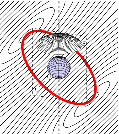
Figure 1: A sketch of the geometrical situation which is discussed in this paper: the black-hole horizon is represented by the sphere $H$ around which the magnetic field is generated by remote sources, e.g. the current loop $L$. It resembles an asymptotically uniform field within some restricted volume (indicated by the rectangle) around the black hole. In general, the magnetic field can be inclined with respect to the rotation axis of the hole (dashed line). The shape of the field lines and the corresponding magnetic flux across the surface $S$ (or any other space-like surface) can be easily determined if the direction of the field coincides with the rotation axis of the hole (an aligned field). But with non-aligned fields and very near the horizon the situation becomes much more complicated.

We consider two different situations hereafter: first, the fields parallel to the rotation axis of the black hole (aligned fields), and then those which are oblique. While the aligned fields are not wound up around the hole (there is no plasma which could induce a toroidal component of the field), the oblique fields are indeed dragged due to the hole’s gravomagnetic influence. The two cases are thus qualitatively different. The main simplification of the former one stems from the fact that the aligned electromagnetic field obeys identical symmetries as the gravitational field.

3 Field lines and fluxes

The general definition of the magnetic and the electric fluxes should reflect the intuitive idea that the flux amounts to the number of field lines crossing the unit surface area at perpendicular orientation, taking into account the observer dependence of the field lines. Since the flux is a scalar quantity, it enables us to define surfaces of constant flux in appropriate way with the corresponding field lines lieing within these surfaces.

Let us consider an arbitrary two-dimensional spacelike surface ${S}$ around the black hole (Figure 1). Such a surface can represent, e.g., a part of a constant radius sphere in spheroidal coordinates $r$, $\theta$, $\phi$. The magnetic and the electric fluxes across the surface, ${\Phi_{\rm{m}}}$ and ${\Phi_{\rm{e}}}$ respectively, are defined by

$${\Phi_{\rm{m}}}=\int_{{S}}\mbox{\bf{F$\wedge$d}}{{S}},\quad{\Phi_{\rm{e}}}=\int_{{S}}\mbox{\bf{${}^{*}\!$F$\wedge$d}}{{S}},$$ (1)

where F denotes the electromagnetic-field 2-form, ${}^{*}\!$F is its Hodge-dual with respect to the spacetime metric, and $\mbox{\bf{d}}{S}$ refers to the element of surface embedded in the four-dimensional spacetime. The symbol $\wedge$ denotes the wedge product of the two forms; see §2 of Bičák & Janiš (1980) for further details. In particular, if ${S}$ is a part of the $r={\rm{const}}$ sphere, then ${\Phi_{\rm{m}}}=\int{}F_{\theta\phi}\,{\rm{d}}\theta\,{\rm{d}}\phi$, which is a natural formula for the magnetic flux where $F_{\theta\phi}$ has the meaning of the radial component of the magnetic field. In the case of a closed surface ${S}$, by applying the Gauss theorem, the integral ${\Phi_{\rm{m}}}$ must vanish (no magnetic charges) while the integral ${\Phi_{\rm{e}}}$ is then proportional to the total electric charge contained in the volume enclosed by ${S}$.

Maxwell’s equations in vacuum can be written in compact form

$$\mbox{\bf{dF}}=0,\quad\mbox{\bf{d${}^{*}\!$F}}=0,$$ (2)

where the operator d denotes exterior differentiation in curved spacetime. The general form of the solution of eqs. (2) can be expressed only in terms of infinite expansions (sum of the multipoles), subject to boundary conditions, but explicit expressions have been found for special cases, namely, the asymptotically uniform magnetic field (King et al.1975). Even such a highly simplified solution becomes rather complicated when the field is not aligned exactly with the rotation axis of the hole, as we illustrate below.

Now we employ the above-given definitions and introduce the concept of surfaces of constant flux. For simplicity, let us start with the fields which are axially symmetric. In this case the black hole behaves like an aligned rotator: once it is placed in the uniform magnetic field, the hole distorts the original structure of the magnetic field and it induces electric fields.

3.1 Axisymmetric fields

    

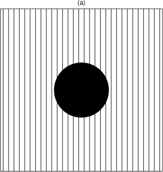
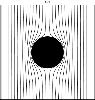
Figure 2: Surfaces of constant flux ${\Phi_{\rm{m}}}$ for the axisymmetric magnetic field. Here we plot the intersections of these cylindrical surfaces with the azimuthal plane $\phi={\rm{const}}$. The black-hole horizon is denoted by a circle, the rotation axis is vertical. Two cases are shown: (a) $a=0$ (a static black hole), and (b) $a=M$ (a maximally rotating black hole). Notice that rapidly rotating holes exhibit the Meissner-type effect (expulsion of the magnetic field out of super-conducting bodies). Only a small region is shown near the horizon, where the effect of the black hole is apparent.

The gravitational field of a black hole in steady rotation possesses two evident symmetries which are crucial in our discussion. These are stationarity and axial symmetry. As a consequence of the symmetries one can employ spheroidal coordinates in which the horizon of the hole is located at constant radius, $r=r_{+}$, and all partial derivatives with respect to azimuth $\phi$ and time $t$ vanish. Due to rotation, however, the gravitational field is not spherical and it depends on the latitudinal coordinate $\theta$ (see the Appendix). The radius of the horizon is given in terms of the black hole’s mass $M$ and its specific angular momentum $a$: $r_{+}=M+\surd(M^{2}-a^{2})$. Rotation of the hole cannot be arbitrarily large and it is limited by the maximum value of the angular momentum, $a=M$ in geometrized units.

The electromagnetic field may or may not possess the same symmetries as the gravitational field. Naturally, the problem is greatly simplified by assuming axial symmetry and stationarity for both fields. We start by examining the asymptotically (i.e. far from the hole) uniform magnetic field which is aligned with the rotation axis and satisfies the required symmetries automatically (Wald 1974). Let us specify the surface ${S}$ as part of the sphere $r={\rm{}const}\geq{}r_{+}$ with the circular boundary given by $\theta={\rm{}const}$ (Fig. 1). Using eq. (1) and the field components from the Appendix one can calculate the fluxes. Denoting the asymptotical strength of the magnetic field by $B_{\parallel}$ we find for the magnetic flux ${\Phi_{\rm{m}}}(r,\theta;a,M,B_{\parallel})$ across the cap ${S}$:

$${\Phi_{\rm{m}}}=\pi{B_{\parallel}}\left[\Delta+\frac{2Mr}{\Sigma}\left(r^{2}-a^{2}\right)\right]\sin^{2}\theta,$$ (3)

where $\Delta=r^{2}-2Mr+a^{2}$, $\Sigma=r^{2}+a^{2}\cos^{2}\theta$. Furthermore, setting ${\Phi_{\rm{m}}}=C={\rm{}const}$, and solving for $r{\equiv}r_{{}_{C}}(\theta)$ one finds a surface of constant flux. Eq. (3) with $r=r_{+}$, $\theta=\pi/2$ can be reduced to eq. (27) of Bičák & Janiš (1980) for the flux of an aligned magnetic field across the hemisphere.

A set of constant-flux surfaces can be parametrized by the values of $C$, where each of the surfaces forms a flux tube with topology of a cylinder along the rotation axis. In other words, $r_{{}_{C}}(\theta)$ determines the poloidal shape of the flux-tube boundary (i.e. its intersection with a $\phi={\rm{const}}$ plane). In particular, one can start by calculating the flux across the whole hemisphere (i.e. one half of the surface of the horizon, $r=r_{+}$ and $\theta\leq\pi/2$), and then, using the same value of ${\Phi_{\rm{m}}}(r_{+},\pi/2)\equiv\Phi_{\rm{}max}$ one proceeds to higher $r$’s up to spatial infinity, $r\rightarrow\infty$. In this way one finds the effective cross-sectional area for the capture of the magnetic flux which is a circle of radius $2M\surd[1-a^{2}/(Mr_{+})]$. This circle is a section of the magnetic flux tube which comes from spatial infinity ($r\rightarrow\infty$, $\sin\theta\rightarrow 0$, where the field is strictly uniform) and eventually crosses the black-hole horizon.

In the non-rotating case, the cross-section is just a circle of radius $r_{+}(a=0)=2M$ while the maximum flux is $\Phi_{\rm{}max}={\pi}B_{\parallel}{r_{+}^{2}}$. But the flux across the hole decreases with $a$ increasing, and in the maximally rotating case ($a=M$) the field becomes expelled out of the hole completely (Bičák & Janiš 1980). In other words, the cross-section shrinks to zero. This conclusion corresponds to ${\Phi_{\rm{m}}}(r=r_{+},a=M)=0$ [cf. eq. (3)], and in this sense the horizon of the maximally rotating black hole bears properties of superconducting bodies, which do not permit external magnetic fields to thread their surfaces.

Two special cases are shown in Figure 2. First, for a non-rotating black hole ($a=0$), the surfaces of constant flux appear indeed as cylinders, $r\sin\theta={\rm{const}}$. The exact shape of cylindrical surfaces of course depends on the choice of the radial coordinate, which is not unique. Unlike angular coordinates which are defined straightforwardly, one could make a transformation $R\equiv{R(r)}$. Such a transformation would introduce a distortion to the lines which came out straight in Fig. 2a. Radius $r$ has a clear meaning far from the black hole where the spacetime becomes flat and $r$ is simply the spherical radial coordinate.

Now we consider the magnetic field lines which, by definition, lie in the surfaces of constant flux and determine the direction of Lorentz force acting on charged particles. Such lines of force are observer dependent (the Lorentz force depends on the particle’s velocity). One thus has to be careful in the choice of preferred observers whose motion defines the lines that are plotted in graphs. In practice one often chooses a frame connected to observers matching in some natural manner the spacetime properties. For example, one can build the frame by requiring that it corotates with the black hole around its axis at such a velocity that the azimuthal component $p_{\phi}$ of energy-momentum four-vector is zero ($\ell=p_{\phi}$ is constant of motion, hence the name for observers attached to this frame: zero angular momentum observers). Another possibility would be to connect the frame with photons ingoing into the hole. We will explore both options hereafter.

    

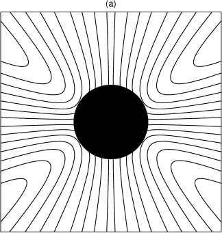
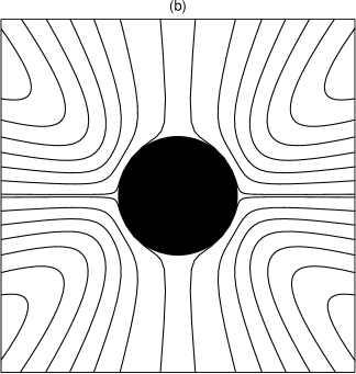
Figure 3: The electric field can be induced by the rotating black hole. In this figure, electric lines of force are plotted corresponding (a) to the uniform aligned magnetic field near the fast rotating black hole ($a=0.95M$); (b) to a similar situation near the maximally rotating hole ($a=M$, as in Fig. 2b).

With aligned fields our task is quite simple (Christodoulou & Ruffini 1973). The lines indicating the shape of the constant flux surfaces in Fig. 2 are parallel to the magnetic force acting on (hypothetical) magnetic monopoles connected with zero angular momentum observers. This can be verified directly from the expression for the acceleration of a particle due to the Lorentz force,

$$m\dot{\mbox{\bf{u}}}=q_{\rm{m}}\mbox{\bf{${}^{*}\!$F.u}},$$ (4)

where on the left-hand side the dot denotes total derivative with respect to particle’s proper time, $m$ and $q_{\rm{m}}$ are its mass and magnetic charge respectively; u is the four-velocity of the inertial reference frame coinciding at each point with the frame of zero angular momentum observers (the first choice of preferred observers mentioned above). The field lines are given by the ordinary differential equation

$$\frac{{{\rm{d}}{r}}}{{{\rm{d}}\theta}}=\frac{B_{r}}{B_{\theta}},$$ (5)

where $B_{r}={{}^{*}\!F}_{r\nu}\,u^{\nu}$, $B_{\theta}={{}^{*}\!F}_{\theta\nu}\,u^{\nu}$ are the magnetic field intensity components calculated by projecting the tensor ${{}^{*}\!F}_{\mu\nu}$ onto the observer’s four-velocity.

The electric fluxes and field lines can be introduced in a similar manner; one only needs to interchange the electromagnetic field tensor by its dual, the magnetic charge by the electric charge, and vice versa wherever they appear in the above-given formulae. The electric field induced by rotation of the hole is shown in Figure 3. (The black hole could have also its own electric charge, giving rise to the Coulomb field which would then have to be superposed to the induced field; but this is just a minor complication.) It is evident that the induced electric field vanishes in the non-rotating case, but quite unapparent is the form of the induced field in Fig. 3, almost radial far from the hole. Based on the classical analogy with a rotating sphere, one would perhaps expect a quadrupole-type component, but here the leading term of the electric field arises due to gravomagnetic interaction which is a purely general-relativistic effect (Ciufolini & Wheeler 1995). This electric field falls off radially as $r^{-2}$.

3.2 Oblique fields

Now we explore the magnetic field which is not aligned with the rotation axis, though it still remains asymptotically uniform (Bičák & Janiš 1980). Let us recall that we are dealing with the test-field solution (linearized in the field intensity) which can be written as a sum of two parts: the first one conveys the contribution of the aligned component as introduced in the previous section (proportional to $B_{\parallel}$), and the second one corresponds to more complicated asymptotically perpendicular field (${\propto}B_{\perp}$). We turn our attention to this second part.

The lines of asymptotically perpendicular field do not reside in one plane and it is not easy to visualize them. The equatorial plane $\theta=\pi/2$ is an exception (for obvious reasons of symmetry) and we thus start here by plotting the lines which are defined in a manner analogous to eq. (5):

$$\frac{{\rm{d}}{r}}{{\rm{d}}\phi}=\frac{B_{r}}{B_{\phi}}.$$ (6)

The lines remain in the equatorial plane ($B_{\theta}=0$ there) but they do not look straight at all. Instead, the lines are wound up by rotation of the hole whenever $a\neq 0$ (Figure 4a), and these dragging effects are progressively enhanced near horizon. The reason of this behaviour is easy to understand, and it is related to the choice of the reference frame. Zero angular momentum observers, to which we attach the frame, circulate around the hole at constant radius; therefore, they experience a rapidly increasing gravitational pull when $r{\rightarrow}r_{+}$ and must be supported by force which eventually diverges at $r=r_{+}$. There the frame becomes nonphysical in the sense that it cannot be realized by any kind of physical particles. A question arises naturally: Can we go over to another frame which does not suffer from such a drawback? This new frame should remain physical everywhere outside the black hole, including the horizon itself.

    

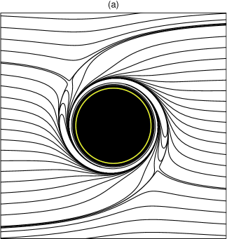
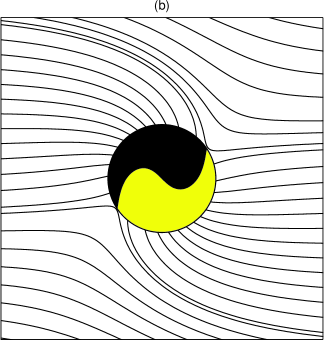
Figure 4: Lines of the magnetic field which is asymptotically uniform and perpendicular to the rotation axis. The equatorial plane is shown as viewed from top, i.e. along the rotation axis, (a) in the frame of zero angular momentum observers orbiting at constant radius; (b) in the frame of freely falling observers. In the panel (b), two regions of ingoing/outgoing lines are distinguished by different levels of shading of the horizon. The hole rotates counter-clockwise ($a=M$).

Let us now transform the field to the frame which is connected to photons falling into the hole straight along latitudinal rays $\theta$ constant. In other words, the infall is simply radial at large distance. Such a frame must remain physical also on the horizon by its very definition: it is realized with the help of particles, motion of which is governed by the hole’s gravity (we could use with similar results also particles of nonzero rest mass instead of photons). Figure 4b shows the magnetic field lines constructed in this frame, sometimes called the Kerr ingoing frame (cf. Appendix). It is evident from the figure that the observers do not experience any particular effects related to the magnetic field structure in the infalling frame near the horizon.

Besides the field lines, we have indicated (by light shading) that part of the horizon where the field enters the hole (the radial component of the local magnetic field is negative there). Integrating over this area one obtains the total ingoing magnetic flux, $\Phi_{\rm{}max}$, which again depends on the rotation parameter $a$, but now in a way substantially different than it was for the aligned fields. We could not derive an analytical formula for the non-aligned flux but we calculated numerically that, e.g., for $a=0.95\,M$ the maximum flux reaches $\Phi_{\rm{}max}\dot{=}5.1B_{\perp}r_{+}^{2}$. This value is larger than the corresponding $\Phi_{\rm{}max}={\pi}B_{\parallel}r_{+}^{2}$ in the aligned case. Moreover, the ingoing flux does not vanish even when $a=M$.

We remark that our total ingoing flux $\Phi_{\rm{}max}$ exceeds the maximum flux across a hemisphere, $\tilde{\Phi}_{\rm{}max}=B_{\perp}{\pi}r_{+}^{2}\surd[1+a^{2}(1+r_{+})^{2}/r_{+}^{4}]$. (The latter formula for $\tilde{\Phi}_{\rm{}max}$ corresponds to eq. (33) of Bičák & Janiš (1980) after correcting their term under the square root.) The reason of the difference between $\Phi_{\rm{}max}$ and $\tilde{\Phi}_{\rm{}max}$ is evident from Fig. 4b: the shaded surface where the flux enters into the horizon does not coincide in shape with a hemisphere. It is $\Phi_{\rm{}max}$ which determines the flux connecting the horizon to distant regions outside the hole, while $\tilde{\Phi}_{\rm{}max}$ is not suitable for this purpose because an inclined hemisphere on the rotating black-hole horizon always contains the regions of both ingoing and outgoing field lines. However, the difference is very small between the two quantities.

By Maxwell equations the ingoing flux is balanced by the outgoing one, so that the total magnetic charge of the hole vanishes. What appears less obvious is the fact that, for some observers, there exist closed loops of magnetic lines which start from the horizon, make a turn, and plunge back into the horizon. This is not the case of the infalling frame, but it can be observed by zero angular momentum observers near the horizon (see Fig. 4a). For them the magnetic flux connecting the hole with distant spatial regions is somewhat less than the maximum ingoing flux on the horizon. Let us note that the field lines connecting the hole with distant regions are relevant for astrophysical problems, since they can establish a link with surrounding plasma and transfer torques between the hole and the plasma.

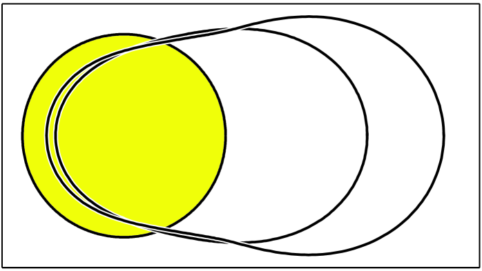
Figure 5: Cross-sectional area for the capture of magnetic field lines (asymptotically uniform magnetic field perpendicular to the rotation axis). The three curves correspond to different values of the black-hole angular momentum: $a=0$ (cross-section is the perfect circle; its projection coincides with the black-hole horizon, indicated here by shading), $a=0.95\,M$, and $a=M$ (the most deformed shape refers to the maximally rotating case).

At this point a comment is worth regarding the choice of the two frames which we have employed. Although there is an infinite number of possible choices, depending on the motion of preferred observers to which the frame is connected, the main difference stems from the fact that $r={\rm{const}}$ observers are kept above the black hole with the help of some supporting force, e.g. by using a thruster rocket (even very close to horizon where the required support increases tremendously) while freely moving observers are allowed to fall in.

The capture of the magnetic flux by the black hole can be characterized by the cross-sectional area also in the case of oblique magnetic fields. The cross-section is defined in much the same way as for the aligned field (see previous section). However, when deriving eq. (3) we took the advantage of axial symmetry: each flux tube of the aligned field had a circular cross-section, while for non-aligned fields the sections are deformed, and their shape remains unknown until the field lines are found.

Hence, for the asymptotically perpendicular field we could not find the shape of flux tubes analytically, although the field lines can still be traced numerically even outside the equatorial plane. One finds the flux tube defining the cross section by shooting from spatial infinity the field lines with a given inclination to the hole’s axis of rotation. Numerically constructed lines were used to determine the cross-sectional area of the hole for the capture of the non-aligned magnetic field. In this way the effective cross-section is obtained in Figure 5 by tracing in a fine grid those field lines that are just on the verge between hitting the hole and missing it. We used the magnetic lines in the ingoing frame to construct this plot. Notice how the cross-sectional area is deformed and enlarged by increasing the angular momentum of the hole.

4 Conclusions

We explored the surfaces of constant magnetic flux and the field lines of the uniform magnetic field near rotating black holes. The test-field solution which we used is simple enough to exhibit the frame-dragging effects in a crystal-clear form. In addition to that, one can show, by expanding the field around the hole into multipoles, that the leading component (the one which dominates near the horizon) corresponds just to this asymptotically uniform field. We observed how the magnetic field in vacuum is dragged and twisted by pure gravitational effects of the hole. When plasma is also present, this effect can lead to rapid reconnection of the field lines, resulting thus in flaring and explosive releases of energy (Mestel 1999). But even the vacuum fields are relevant in astrophysics. It has been suggested (Tomimatsu 2000) that they can act as seeds for the dynamo process, which subsequently amplifies the magnetic fields in rotating magnetospheres of compact objects.

The possibility of extracting the rotational energy via the magnetic field requires that the field threads the horizon. Bičák & Janiš (1980) remarked that the efficiency of this process may be seriously limited by the magnetic-field expulsion if the hole rotates very rapidly, but this constraint applies only to the field which is uniform and aligned. As we illustrated in previous section, non-aligned fields thread the horizon even in the case of extreme rotation, and the complicated structure of the field suggests that significant acceleration of particles takes place due to reconnection of the field lines near the horizon.

The problem of magnetic fluxes threading black holes has also other astrophysically relevant implications. The fields around rotating holes are of particular interest because the newly born holes probably gain a lot of angular momentum at the moment of creation by violent contraction. Magnetic fields could extract rotational energy from the black hole back by converting it to the outflowing Poynting flux and to kinetic energy of accelerated plasma flows (Blandford & Znajek 1977; for recent accounts of the problem, see Punsly 1996; Ghosh & Abramowicz 1997). Indeed, such outflows are observed, but the regions where they originate remain below resolution capabilities of present-day techniques.

As still another exciting application, it has been proposed that the energy of the electromagnetic field is violently released in some transient types of astronomical objects. The process could start if a massive torus is formed as a relic of a close encounter between two neutron stars, one of them being disrupted by tidal forces exerted by its companion. The orbiting matter then undergoes the gravitational collapse into the black hole due to a certain kind of rapid instability (Daigne & Mochkovitch 1997; Abramowicz et al. 1998). If the magnetic field were initially held by the torus (as we sketched in Fig. 1) then its collapse would increase the magnetic intensity tremendously (due to the flux conservation) while subsequent disappearance of the torus leads to the lack of this support and to sudden expansion of the field lines. Rapid acceleration of the surrounding plasma results thereof, and eventually a burst of radiation is produced. Similar processes have been proposed as a possible origin of gamma-ray bursts (Hanami 1997; Daigne & Mochkovitch 2000; Lee et al. 2000), powerful and as yet unexplained events which are routinely detected by specialized satellites.

The authors thank the referee for helpful comments which helped us to improve our text. MD and VK acknowledge support from the grants GA CR 205/00/1685 and GA UK 63/98 in the Czech Republic.

Appendix

Gravitational field of a rotating black hole is described by Kerr metric. In this Appendix we summarize the relevant expressions for the spacetime metric, for the structure of weak electromagnetic fields around the hole, and for the electric and the magnetic lines.

The spacetime metric and the electromagnetic field

Kerr metric has the form (Misner et al. 1973, chapt. 33)

$$\fl{\rm d}s^{2}=-\Delta\Sigma{{\cal A}^{-1}}\,{{\rm{d}}}t^{2}+\Sigma\Delta^{-1}\,{{\rm{d}}}r^{2}+\Sigma\,{{\rm{d}}}\theta^{2}+{\cal A}\Sigma^{-1}\sin^{2}\theta\;\left({\rm{d}}\phi-\omega\,{{\rm{d}}}t\right)^{2};$$ (A.1)

here, spheroidal (Boyer-Lindquist) coordinates, $x^{\mu}\equiv\{t,r,\theta,\phi\}$, and geometrized units ($c=G=1$) have been used, $M$ and $a$ denote the mass and the specific angular momentum of the body, $\Delta(r)=r^{2}-2Mr+a^{2}$, $\Sigma(r,\theta)=r^{2}+a^{2}\cos^{2}\theta$, ${\cal A}(r,\theta)=(r^{2}+a^{2})^{2}-{\Delta}a^{2}\sin^{2}\theta$, and $\omega(r,\theta)=2Mar/\cal{A}$. Notice that on the horizon $\Delta(r_{+})=0$.

The electromagnetic field tensor F can be expressed in terms of the four-potential, $\mbox{\bf{F}}=\mbox{\bf{dA}}$. Spelling out the components explicitly, one obtains

$$F_{\mu\nu}=\frac{\partial{A_{\nu}}}{\partial{x^{\mu}}}-\frac{\partial{A_{\mu}}}{\partial{x^{\nu}}},$$ (A.2)

where (eq. (A4) of Bičák & Janiš 1980)

$$\fl A_{t}=B_{\parallel}a\left[Mr\Sigma^{-1}\left(1+\cos^{2}\theta\right)-1\right]+B_{\perp}aM\Sigma^{-1}\Psi\sin\theta\cos\theta,$$

$$\fl A_{r}=-B_{\perp}(r-M)\sin\theta\cos\theta\sin\psi,$$

$$\fl A_{\theta}=-B_{\perp}\Big{[}\left(r\sin^{2}\theta+M\cos^{2}\theta\right)a\cos\psi+\Big{(}r^{2}\cos^{2}\theta+\left(a^{2}-Mr\right)\cos 2\theta\Big{)}\sin\psi\Big{]},$$

$$\fl A_{\phi}=B_{\parallel}\left[{\textstyle\frac{1}{2}}\left(r^{2}+a^{2}\right)-a^{2}Mr\Sigma^{-1}\left(1+\cos^{2}\theta\right)\right]\sin^{2}\theta$$

$$\lo-B_{\perp}\left[\Delta\cos\psi+\left(r^{2}+a^{2}\right)M\Sigma^{-1}\Psi\right]\sin\theta\cos\theta,$$

$\psi=\phi+a\delta^{-1}\ln\left[\left(r-r_{+}\right)/\left(r-r_{-}\right)\right]$, $\Psi=r\cos\psi-a\sin\psi$, $\delta=r_{+}-r_{-}$, $r_{\pm}=M\pm\sqrt{M^{2}-a^{2}}$.

The field lines

The components of electric and magnetic intensities, $E_{(k)}$ and $B_{(k)}$, measured by a physical observer (i.e., for example, experienced by a charged particle) can be obtained by projecting $F_{\mu\nu}$ and its dual onto the local tetrad of basis vectors $\mbox{\bf{e}}_{(k)}$,

$$E_{(k)} = \mbox{\bf{e}}_{(k)}^{\mu}F_{\mu\nu}\,u^{\nu}=F_{(k)(t)},$$ (A.3)

$$B_{(k)} = {\mbox{\bf{e}}_{(k)}^{\mu}}{{}^{*}\!F}_{\mu\nu}\,u^{\nu}={{}^{*}\!F}_{(k)(t)},$$ (A.4)

where $u^{\nu}\equiv\mbox{\bf{e}}_{(t)}^{\nu}$ is the observer’s four-velocity, and the remaining three basis vectors are chosen as space-like, mutually perpendicular vectors. In particular, we have used the frame of radially infalling photons. The tetrad defining this frame is obtained by transforming the time and the azimuthal angle, $\{t,\phi\}\rightarrow\{v,\psi\}$, in the following way: $\mbox{\bf{d}}v=\mbox{\bf{d}}t+\left(r^{2}+a^{2}\right)\Delta^{-1}\mbox{\bf{d}}r$, $\mbox{\bf{d}}\psi=\mbox{\bf{d}}\phi+a\Delta^{-1}\mbox{\bf{d}}r$ (Kerr ingoing coordinates). Here, indices $(k)$ in round parentheses correspond to spatial coordinates $(r)$, $(\theta)$, $(\phi)$.

Notice that, in an orthonormal tetrad, one can shift spatial indices of a tensor up and down without any change, while the sign of each tensorial quantity must be changed when shifting the time index $(t)$.

Coordinate components of the electric and the magnetic intensities (A.3)–(A.4) are

$$E^{\mu} = {F^{\mu}}_{\nu}\,u^{\nu}={e_{(k)}}^{\mu}E^{(k)}\,,$$ (A.5)

$$B^{\mu} = {{}^{*}\!F^{\mu}}_{\nu}\,u^{\nu}={e_{(k)}}^{\mu}B^{(k)}\,.$$ (A.6)

Under the Lorentz force, the motion of electrically/magnetically charged test particles obeys equations

$$m\,a^{\alpha}=q_{\rm{e}}\,{F^{\mu}}_{\nu}\,u^{\nu},\quad m\,a^{\alpha}=q_{\rm{m}}{{}^{*}\!F^{\mu}}_{\nu}\,u^{\nu},$$ (A.7)

respectively (cp. eq. (4)). Here, $m$ is the mass of the particle and $a^{\alpha}=u^{\alpha}_{;\beta}\,u^{\beta}$ is four-acceleration.

The electric and the magnetic lines are determined by the differential equations

$$\frac{{\rm d}x^{\mu}}{{\rm d}s}=E^{\mu},\,\quad\frac{{\rm d}x^{\mu}}{{\rm d}s}=B^{\mu}\,.$$ (A.8)

The shape of the lines depends on the choice of the particular frame and coordinates which are used to draw the curves.

Two examples of the tetrads

As an example, we can write the explicit form of the tetrads mentioned in the text (for a useful summary of their properties and for further details, see Semerák 1993). The tetrad of zero angular momentum observers is in Boyer-Lindquist coordinates

$$\mbox{\bf{e}}_{(t)} = {\cal A}^{1/2}\left(\Delta\Sigma\right)^{-1/2}\,\mbox{\bf{[}}1,0,0,\omega\mbox{\bf{]}}\,,$$ (A.9)

$$\mbox{\bf{e}}_{(r)} = \mbox{\bf{[}}0,\Delta^{1/2}\Sigma^{-1/2},0,0\mbox{\bf{]}}\,,$$ (A.10)

$$\mbox{\bf{e}}_{(\theta)} = \mbox{\bf{[}}0,0,\Sigma^{-1/2},0\mbox{\bf{]}}\,,$$ (A.11)

$$\mbox{\bf{e}}_{(\phi)} = \mbox{\bf{[}}0,0,0,{\cal A}^{-1/2}\Sigma^{1/2}\sin^{-1}{\!\theta}\mbox{\bf{]}}\,.$$ (A.12)

Observers at rest with respect to the tetrad (A.9)–(A.12) follow an orbit with $r$, $\theta$ constant, and with angular momentum $\ell=0$. Notice that these observers are accelerated rather than freely falling.

For the tetrad attached to observers at free fall (along $\theta={\rm{const}}$ from the rest at infinity) one obtains

$$\hat{\mbox{\bf{e}}}_{(t)} = \Sigma^{-1}\mbox{\bf{[}}1-(r^{2}+a^{2}){\cal K},-[2Mr(r^{2}+a^{2})]^{1/2},0,-a{\cal K}\mbox{\bf{]}}\,,$$ (A.13)

$$\hat{\mbox{\bf{e}}}_{(r)} = {\cal A}^{1/2}\Sigma^{-1}\,\mbox{\bf{[}}1-{\cal K},1,0,a{\cal A}^{-1}\Sigma+\omega(1-{\cal K})\mbox{\bf{]}}\,,$$ (A.14)

$$\hat{\mbox{\bf{e}}}_{(\theta)} = \mbox{\bf{[}}0,0,\Sigma^{-1/2},0\mbox{\bf{]}}\,,$$ (A.15)

$$\hat{\mbox{\bf{e}}}_{(\psi)} = \mbox{\bf{[}}0,0,0,{\cal A}^{-1/2}\Sigma^{1/2}\sin^{-1}{\!\theta}\mbox{\bf{]}}\,,$$ (A.16)

where ${\cal K}(r)=\left[1+(2Mr)^{-1/2}(r^{2}+a^{2})^{1/2}\right]^{-1}$.

Abramowicz M A, Karas V, Lanza A 1998 “On the runaway instability of relativistic accretion tori”, Astron. Astrophys. 331 1143–46

Asseo E, Sol H 1987 “Extragalactic magnetic fields”, Phys. Rep. 148 307–436

Bičák J, Janiš V 1980 “Magnetic fluxes across black holes”, Mon. Not. Roy. Astron. Soc. 212 899–915

Blandford R D, Znajek R 1977 “Electromagnetic extraction of energy from Kerr black holes”, Mon. Not. Roy. Astron. Soc. 179 433-56

Bullard E C 1949 “Electromagnetic induction in a rotating sphere”, Proc. Roy. Soc. Lond. 199 413–41

Christodoulou D, Ruffini R 1973 “On the electrodynamics of collapsed objects”, in Black Holes, eds C DeWitt & B S DeWitt (New York: Gordon and Breach Science Publishers) p R151

Ciufolini I, Wheeler J A 1995 Gravitation and Inertia (New Jersey: Princeton University Press)

Daigne F, Mochkovitch R 1997 “Gamma-ray bursts and the runaway instability of thick discs around black holes”, Mon. Not. Roy. Astron. Soc. 285 L15–19

Daigne F, Mochkovitch R 2000 “Mass loss from a magnetically driven wind emitted by a disk orbiting a stellar mass black hole”, in Proceedings of the 5th Huntsville Gamma-Ray Burst Symposium (Huntsville 1999), in press; astro-ph/9912444

Duncan R C, Thompson C 1992, “Formation of very strongly magnetized neutron stars”, Astrophys. J. Lett. 392 L9–13

Ghosh P, Abramowicz M A 1997 “Electromagnetic extraction of rotational energy from disc-fed black holes”, Mon. Not. Roy. Astron. Soc. 292 887–95

Goldreich P, Julian W H 1969 “Pulsar electrodynamics”, Astrophys. J. 157 869–80

Hanami H 1997 “Magnetic cannonball model for gamma-ray bursts”, Astrophys. J. 491 687–96

Herzenberg A, Lowes F J 1957 “Electromagnetic induction in rotating conductors”, Phil. Trans. Roy. Soc. Lond. 249 507–84

Hewish A et al. 1968 “Observation of a rapidly pulsating radio source”, Nature 217 709–13

Jackson J D 1975 Classical Electrodynamics (New York: Wiley)

King A R, Lasota J P, Kundt W 1975 “Black holes and magnetic fields”, Phys. Rev. D 12 3037–42

Kouveliotou C et al. 1998 “An X-ray pulsar with a superstrong magnetic field in the soft gamma-ray repeater SGR 1806-20”, Nature 393 235–37

Kronberg P P 1994 “Extragalactic magnetic fields”, Rep. Prog. Phys. 57 325

Krotkov R V, Pellegrini G N, Ford N C, Swift A R 1999 “Relativity and the electric dipole moment of a moving, conducting, magnetized sphere”, Am. J. Phys. 67 493–98

Lee H K, Wijers R A M J, Brown G E 2000 “The Blandford-Znajek process as a central engine for gamma-ray bursts”, Phys. Rep. 325 83–114

Mestel L 1999 Stellar Magnetism (Oxford: Clarendon Press)

Michel F C, Hui Li 1999 “Electrodynamics of neutron stars”, Phys. Rep. 318 227–97

Mihara T et al. 1990 “New observations of the cyclotron absorption feature in Hercules X-1”, Nature 346 250–52

Misner C W, Thorne K S, Wheeler J A 1973 Gravitation (New York: W H Freeman & Co)

Miyama S M, Tomisaka K, Hanawa T (eds) 1999 Numerical Astrophysics (Boston: Kluwer Academic Publishers)

Murakami T et al. 1988 “Evidence for cyclotron absorption from spectral features in gamma-ray bursts seen with Ginga”, Nature 335 234–35

Pacini F 1967 “Energy emission from a neutron star”, Nature 216 567–68

Punsly B 1996 “Fast Waves and the Causality of Black Hole Dynamos” Astrophys. J. 467 105–25

Semerák O 1993 Gen. Rel. Grav. 25 1041

Thorne K S, Price R H, Macdonald D A 1986 Black Holes: The Membrane Paradigm (New Haven: Yale University Press)

Tomimatsu A 2000 “Relativistic dynamos in magnetospheres of rotating compact objects”, Astrophys. J. 528 972–978; astro-ph/9908298

Wald R M 1974 “Black hole in a uniform magnetic field”, Phys. Rev. D 10 1680–85

Zhang B, Harding A C 2000 “High magnetic field pulsars and magnetars: a unified picture”, Astrophys. J. Lett. in press; astro-ph/0004067

Magnetic fluxes across black holes in a strong magnetic field regime V. Karas  and Z. Budínová
Astronomical Institute, Charles University Prague,
V Holešovičkách 2, CZ-180 00 Praha, Czech Republic

PACS numbers: 97.60.Lf, 04.40.Nr

Journal: Physica Scripta 61, 25 (2000)

1 Introduction

The structure of magnetic fields interacting with the gravitational field of a black hole attracted considerable interest in the 1970s, and since then the subject has reached a text-book level [1]–[3]. It is of its own interest and helps to clarify various issues within the framework of the classical Einstein-Maxwell theory, namely the solution-generating techniques in general relativity [4, 5], but the main motivation to study black holes immersed in magnetic fields originates in astrophysics. We know for sure that interstellar and intergalactic magnetic fields do exist and they get amplified in the course of accretion onto compact objects when the field is frozen in plasma and the dynamo effects are involved [6, 7]. However, the energy density contained in realistic magnetic fields, though they can be extremely strong (about $10^{12}$ gauss near neutron stars, and $\approx 10^{15}$ gauss around presumed magnetars [8] and, possibly, in gamma-ray bursters [9]), turns out to be too low to influence the background spacetime metric. Test-field solutions are adequate in such circumstances, and corresponding exact solutions of coupled Einstein-Maxwell equations are mainly the question of principle. The influence of large-scale magnetic fields upon the black-hole metric can be roughly characterized by dimensionless parameter $\beta=B_{0}M$, where $B_{0}$ is the field strength and $M$ is the mass of the object in geometrized units. Considering the above-mentioned limit on the field strength near a one solar-mass magnetar, we obtain $\beta\approx 10^{-5}B_{15}(M/M_{\odot})\ll 1$, where $B_{15}=B_{0}/(10^{15}{\rm{gauss}})$. Such magnetic field contributes substantially to the spacetime metric on spatial scales of $r\approx\beta^{-1}$, as can be easily seen by direct inspection of eq. (1) below. In physical units, this scale implies $r\approx 10^{5}$ km.

Recently, the implications of the classical solutions have been resurrected by several authors within the framework of the string theory. For example, superconducting properties of extremal solitonic objects ($p$-branes) [10] can be related to the expulsion of external, asymptotically uniform magnetic fields from extremal black holes (rotating and electrically charged) in general relativity [11]–[13]. We further discuss this effect for aligned magnetic fields in the next section. (There is apparently a misinterpretation in Sec. V of [10] concerning the expulsion of non-aligned test fields. These fields are not expelled even in the limit of extreme black holes, as can be shown by calculating magnetic fluxes [13] and plotting the lines of magnetic force [14].)

Here we rest on the grounds of classical exact solutions and we deal with the stationary, aligned, asymptotically uniform magnetic fields around magnetized Kerr-Newman (MKN) black holes [15, 16]. Even such simplified solutions are of interest: in a restricted region, they can approximate collapsed objects interacting with the fields, which are generated by remote sources. These calculations are also useful as test-beds for checking numerical solvers. By employing the standard covariant definition of the magnetic flux, otherwise complicated expressions can be illustrated in an intuitive manner. We will observe the expulsion of strong fields out of the horizon, as it occures in the MKN spacetime with vanishing total angular momentum $J$ or vanishing total electric charge $Q$, both quantities being defined in terms of Komar’s integrals [17]–[19]. One can ask whether the magnetic field is, in some natural way, separable into two parts, the first one corresponding to a dipole-type field of the rotating body, and the other one corresponding to the external field (generated by outside sources), which gets expelled when the black hole becomes extreme. In the present paper we show that the aligned and uniform external magnetic field is expelled out of the extreme MKN black hole in the limit of the weak magnetic field, however, similar distinction of the field into the black hole’s dipole-type part and the external part cannot be meaningfully introduced in the strong-field regime.

2 The magnetic flux

2.1 Motivations

Our present subject of the magnetized black holes can be linked to an analogous problem in classical electrodynamics when a rotating sphere is immersed in an external magnetic field. The reason for this analogy stems from the fact that the black hole horizon can be treated as a membrane with effective resistivity. The well-known similarity between these two situations is instructive, and we thus briefly recall several relevant works as the motivation for the present paper. The classical problem was treated in original works by Faraday, Lamb, Thomson and Hertz. More recently, Elsasser [20, 21] and Bullard [22, 23] took interest in the theory of geomagnetic dynamo and examined quasi-stationary solutions for a sphere or concentric spheres with general orientation between rotation axis and the external field. (Non-stationary oscillating electromagnetic fields are far more complicated, and they decay rapidly with the relaxation time-scale which is of the order of light-crossing time across the sphere; corresponding solutions have been discussed also in context of black holes [24].) Geomagnetic applications enable one to ignore higher-order terms in $v^{2}/c^{2}$ and to simplify the problem considerably. Herzenberg & Lowes [25] extended previous works by detailed discussion of special configurations, in particular, these authors examined the dragging of asymptotically misaligned field-lines and their winding up onto a rotating body. Schmutzer [26], in a series of articles, discussed asymptotically uniform stationary magnetic fields interacting with a rotating and electrically conducting sphere, and he derived expressions for the electric charge induced on the surface and for Foucalt currents which, in turn, affect rotation of the sphere. Similar topics were applied to the pulsar astrophysics by Pacini [27] and Goldreich & Julian [28], and then developed by numerous authors till the present [29]. Again, there is analogous winding effect which drags non-aligned fields around black holes [14, 30] and gives rise to fictitious induced charges and currents on the horizon [31]–[33]. Astrophysically realistic pulsar magnetospheres are more complicated, however, because in this case one cannot assume the electrovacuum condition.

The special-relativity terms were examined by several authors. Bladel [34, 35] performed standard but tedious expansions in small parameter $v/c$, while Georgiou [36] formulated and solved this problem within the approximation of perfect magnetohydrodynamics which is particularly relevant in astrophysics. Numerical codes dealing with general-relativistic magnetohydrodynamics have been developed and applied to the problem of astrophysical accretion and jets [38, 39]. Finally, the structure of rotating neutron stars with magnetic fields has been studied within full general relativity [37]. Very strong magnetic fields deform the shape of the star; then, if the field is non-aligned with rotation axis and if the star rotates rapidly, substantial amount of gravitational waves may be produced. In the next section we restrict ourselves to much simpler class of axisymmetric and stationary spacetimes.

2.2 Magnetized black holes

Magnetized Kerr-Newman metric [15] represents an exact electrovacuum solution. In spheroidal coordinates and in the standard notation it has a form

$$\!\!\!\!\!\!\!\!\!\!g=|\Lambda|^{2}\Sigma\left(\Delta^{-1}{\rm{d}}{r}^{2}+{\rm{d}}{\theta}^{2}-\Delta{A^{-1}}{\rm{d}}{t}^{2}\right)+|\Lambda|^{-2}\Sigma^{-1}A\sin^{2}\theta\left({\rm{d}}{\phi}-\omega{\rm{d}}{t}\right)^{2},$$ (1)

where $\Sigma=r^{2}+a^{2}\cos^{2}\theta$, $\Delta=r^{2}-2r+a^{2}+e^{2}$, $A=(r^{2}+a^{2})^{2}-{\Delta}a^{2}\sin^{2}\theta$ are functions from the Kerr-Newman metric, while $\Lambda=1+\beta\Phi-\frac{1}{4}\beta^{2}{\cal{E}}$ is given in terms of the Ernst complex potentials $\Phi(r,\theta)$ and ${\cal{E}}(r,\theta)$:

$$\Sigma\Phi = ear\sin^{2}\theta-{{\rm{i}}}e\left(r^{2}+a^{2}\right)\cos\theta,$$ (2)

$$\Sigma{\cal{E}} = -A\sin^{2}\theta-e^{2}\left(a^{2}+r^{2}\cos^{2}\theta\right)$$ (3)

$$+2{{\rm{i}}}a\left[\Sigma\left(3-\cos^{2}\theta\right)+a^{2}\sin^{4}\theta-re^{2}\sin^{2}\theta\right]\cos\theta.$$

All quantities are expressed in geometrized units and multiplied by suitable power of $M$, so that we deal with dimensionless variables. The explicit form of the metric function $\omega(r,\theta)$ was given in [16] but is not necessary for our discussion of magnetic fluxes. The spacetime (1) is characterized by parameters $a$, $e$, and $\beta$ (angular-momentum parameter, electric-charge parameter, and the magnetic field strength). The most general solution of this type contains additional two parameters characterizing the asymptotic electric field and magnetic charge of the black hole [40], but we do not consider this possibility here.

The electromagnetic field can be written in terms of orthonormal components in the locally non-rotating frame,

$$H_{(r)}+{{\rm{i}}}E_{(r)} = A^{-1/2}\sin^{-1}\!\theta\,\Phi^{\prime}_{,\theta},$$ (4)

$$H_{(\theta)}+{{\rm{i}}}E_{(\theta)} = -\left(\Delta/A\right)^{1/2}\sin^{-1}\!\theta\,\Phi^{\prime}_{,r},$$ (5)

where $\Phi^{\prime}(r,\theta)=\Lambda^{-1}\left(\Phi-\frac{1}{2}\beta{\cal{E}}\right)$. The horizon is located at $r{\equiv}r_{+}=1+\sqrt{(}1-a^{2}-e^{2})$, independent of $\beta$. As in the non-magnetized case, the horizon exists only for $a^{2}+e^{2}\leq 1$, equality corresponding to the extreme configuration. Angular coordinates take the values $0\leq\theta\leq\pi$, $0\leq\phi<2\pi|\Lambda_{0}|^{2}$ where $|\Lambda_{0}|^{2}\equiv|\Lambda(\sin\theta=0)|^{2}=1+\frac{3}{2}\beta^{2}e^{2}+2\beta^{3}ae+\beta^{4}\left(\frac{1}{16}e^{4}+a^{2}\right)$.

Knowing electromagnetic field structure one can calculate the total electric charge $Q_{\rm{H}}$ and magnetic flux $F_{\rm{H}}(\theta)$ across a cap in axisymmetric position on the horizon (with the edge defined by $\theta={\rm{const}}$):

$$Q_{\rm{H}} = -|\Lambda_{0}|^{2}\,\Im{\rm{m}\,}\Phi^{\prime}\left(r_{+},0\right),$$ (6)

$$F_{\rm{H}} = 2\pi|\Lambda_{0}|^{2}\,\Re{\rm{e}\,}\Phi^{\prime}\left(r_{+},\bar{\theta}\right)\Bigr{|}^{\theta}_{\bar{\theta}=0}.$$ (7)

These two quantities are defined invariantly and have been written in different forms and approximations [17]–[19]. It is thus useful to illustrate their properties by plotting graphs which in the end appear very intuitive. Notice that $|\Lambda_{0}|^{2}$ is introduced in eqs. (6)–(7) by rescaling the range of azimuthal coordinate, which is necessary to avoid a conical singularity on symmetry axis [41, 42]. (We allude to this fact because the solution-generation technique guarantees that Einstein-Maxwell equations are satisfied by the spacetime (1)–(5) locally; one has to further determine its global properties.) Given parameters $\beta$, $a$ and $e$, the multiplicative factor $|\Lambda_{0}|$ is constant, independent of $r$. It is thus convenient to rescale the variables containing this factor. We introduce $Q=|\Lambda_{0}|^{-2}Q_{\rm{H}}$ and $F=|\Lambda_{0}|^{-2}F_{\rm{H}}$ which do not contain the square of $|\Lambda_{0}|$.

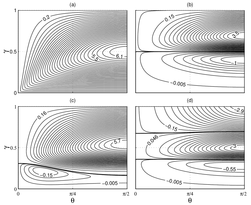
Figure 6: The contour-lines of constant flux $F$ across a cap $\theta={\rm{const}}$ on the horizon for different values of magnetic-field parameter $\gamma(\beta)$. Parameters of the black hole are: (a) $a=e=0$; (b) $a=1$, $e=0$; (c) $a=0.2$, $e=0$; (d) $a=-e=1/\sqrt{2}$. Selected values of $F$ are given with corresponding contours for orientation. See the text for details.

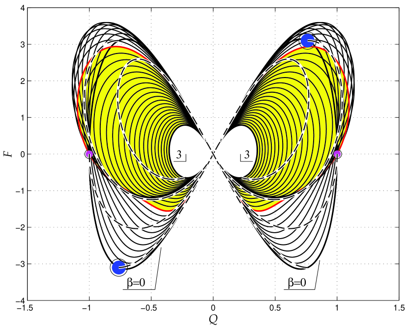
Figure 7: The magnetic flux $F$ of the extreme magnetized Kerr-Newman black hole as a function of its electric charge $Q$. Each solid curve corresponds to a fixed value of $\beta$ within the range $\langle 0,3\rangle$; $\beta=0$ is the case of Kerr-Newman black hole with no external magnetic field. The lines of constant ratio $a/e$ and varying $\beta$ are also plotted (dashed; the cases of $a/e=\pm 0.85$ and $0$ are shown).

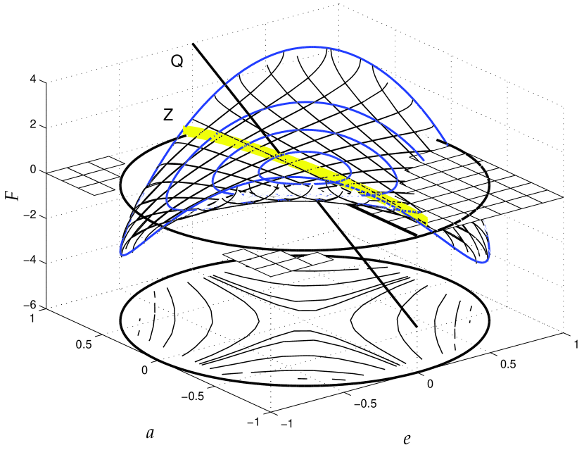
Figure 8: Surface plot of the flux $F$ across the whole hemisphere $\theta=\pi/2$ as function of parameters $a$, $e$. The surface is defined on the circle $a^{2}+e^{2}\leq 1$.

Figure 6 shows contours of constant $F$ in the plane of $\gamma=\left(1+\beta\right)^{-1}$ and $\theta$ (size of the cap). Panels (a)–(d) illustrate the topologically different situations which arise for different combinations of $a$ and $e$. The whole range of $0\leq\theta\leq\pi/2,$ $0\leq\beta(\gamma)\leq\infty$ ($1\geq\gamma\geq 0$) is captured in the four graphs. In particular, setting $\theta=\pi/2$, one obtains the flux across the whole hemisphere. Fig. 6a corresponds to the magnetized Schwarzschild metric ($a=e=0$) while (b) and (d) show two extreme configurations ($a^{2}+e^{2}=1$). One can see in Fig. 6a that the flux reaches maximum of $F=2\pi$ for $\gamma=0.5$, the result which was mentioned (apart from minor numerical errors) in refs. [13] and [17]. In other words, the flux is not a monotonic function of the magnetic-field parameter and it decreases when the field strength exceeds certain value, depending on $a$ and $e$. (It is a monotonic function in the limit of a weak magnetic field only.) It turns out that the flux is, in absolute value, less then $2\pi$ for all other combinations of $a$, $e$. In terms of its $\beta$-dependence, the flux first concentrates to symmetry axis $\theta=0$ when $\beta$ increases from zero to unity, but than it spreads away from the axis. (It was mentioned in ref. [13] that this effect could limit efficiency of the Blandford-Znajek mechanism for electromagnetic extraction of energy from rotating black holes, because its power is proportional to the flux. Characteristic value of $\beta=1$ for which the flux is maximum, however, corresponds to unrealistically strong magnetic fields for currently considered astrophysical applications.) The extreme configurations (b) and (d) are more complicated because the rotating charge of the black hole induces its own contribution to the magnetic flux, and $F$ can even reverse its sign. The black hole’s own contribution to the flux is visible particularly well in Fig. 6d ($a=-e=1/\sqrt{2}$) where the contours intersect abscissa $\gamma=1$. This happens in the Kerr-Newman case with $ae\neq 0$ and no external magnetic field. The flux across any part of the horizon vanishes for certain critical values of $\beta=\beta_{\rm{cr}}(a,e)$, indicated by thick solid lines. For example, $\beta_{\rm{cr}}(1,0)=1$ (cf. Fig. 6b). The exactly horizontal direction of the separatrix corresponds to complete expulsion of the field out of extreme black holes with vanishing charge $Q$ or vanishing angular momentum $J$ [18, 19]. What distinguishes the case (b) from (c) is extremality of the hole. The panel (c) corresponds to the rotating and charged (but not extreme) case; again, the flux vanishes along the separatrix, but the magnetic field still threads the horizon, $H_{(r)}(r=r_{+})\neq 0$, which in this graph means that $\beta_{\rm{cr}}(a,e;\theta)$ depends on the cap’s latitudinal size rather than being constant.

Figure 7 shows the curves of $F(Q)$ across the whole hemisphere $\theta=\pi/2$ in the extreme MKN metric. Such graphs help us to elucidate the behaviour of the flux when $\beta$ is kept fixed while the angular momentum or the electric charge of the hole vary. Each of the closed $\infty$-shaped curves corresponds to different strength of the magnetic field (solid lines), and the part of the graph corresponding to strong magnetic fields, $\beta\geq 1$, is indicated by shading for clarity. The two boundary curves are designated by their corresponding values of $\beta$: “$\beta=0$” and “$3$” in the plot. Naturally, the former one is anti-symmetric with respect to $Q=0$ because there is no contribution to $F$ from external magnetic field. It is only the black hole’s rotating charge which gives rise to the magnetic flux when $\beta=0$. In other words, each two points positioned on the “0” curve anti-symmetrically with respect to origin are related by $ae\rightarrow-ae$ in eq. (7). Two particular cases are designated in the plot: (i) $a=0$, $e=\pm 1$ (small circles), and (ii) $a=0.65$, $e=\pm 0.76$ (large circles). Notice that this feature of anti-symmetrical $F(Q)$ is lost when the magnetic field becomes strong, indicating that it would be difficult to define a natural split of the total field near the horizon into a contribution of the rotating and charged black hole and of the external field. Dashed curves correspond to $a/e={\rm{const}}$. These curves start from a point on the $\beta=0$ solid curve, they proceed through the origin of the plot (where both $Q$ and $F(Q)$ vanish), and terminate at their intersection with the $\beta=3$ curve. The intersection with the line $F=0$ at $Q\neq 0$ corresponds to vanishing angular momentum, $J=0$. For example, the dashed curve starting from the small circle corresponds to the magnetized extreme Reissner-Nordstrøm configuration. In spite of $a=0$, the flux is in general non-zero along this curve in agreement with the fact of non-vanishing $J$.

Figure 8 is a surface plot of $F(a,e)_{|\theta=\pi/2}$ for a fixed value of $\beta=0.05$ (projected contours are shown, too). The surface is restricted by the condition $a^{2}+e^{2}\leq 1$. Four circles of $\sqrt{(}a^{2}+e^{2})=0.25$, 0.5, 0.75, and 1.0 are shown. The shaded band on the surface, denoted by “Z”, indicates where the total electric charge is zero. Obviously, zero charge does not coincide with $e=0$, and, on the other hand, $Q(a,e=0)$ does not vanish and its graph is shown by solid curve “Q”. Here, $\beta$ is small and the curve Q looks almost linear (values are multiplied by factor of 40 for clarity). As we have already mentioned, the flux across the extreme MKN hole vanishes also at other two points where $J$ is zero. These points are near $a=0$ for $\beta\ll 1$, as in this plot. On the other hand, absolute value of $F$ is maximum for $|a|\approx|e|\approx 1/\sqrt{2}$ because the contribution to the flux from the black hole’s rotating charge dominates. The whole picture is qualitatively similar also for higher values of $\beta$: the central part ($a^{2}+e^{2}\mathrel{\hbox to0.0pt{\lower 3.0pt\hbox{$\mathchar 536\relax$}\hss}\raise 2.0pt\hbox{$\mathchar 316\relax$}}0.5$) of the surface, however, is gradually pulled upwards (indicating that the contribution of the hole’s charge becomes less important), and the critical points $Q=0$ and $J=0$ move away from $e=0$ and $a=0$ on the perimeter of the unit circle.

The three above described figures contain complete information about the electric charge of the hole and the magnetic flux threading its horizon.

3 Conclusions

We examined the magnetic fluxes in the MKN spacetime for arbitrary values of parameters $a$, $e$, and $\beta$. The form of the separatrix in contour plots of $F$, as function of $\beta$ and of the polar-cap size $\theta$, illustrates how the field is expelled out of the horizon, and how a balance is established for certain $\beta_{\rm{cr}}(a,e;\theta)$ between the external flux threading the hole and the hole’s own flux, which arises from its rotating charge. Non-monotonic dependence of the flux on $\beta$ can be ascribed to the interplay between two factors. First, the surface of the horizon ${\cal{S}}$ increases sharply with $\beta$ whenever $a$ and/or $e$ are non-zero: ${\cal{S}}=4\pi\left(r^{2}_{+}+a^{2}\right)|\Lambda_{0}|^{2}$. Second, the magnetic field itself influences the flux distribution for high values of $\beta$, as we illustrated by the graphs of magnetic fluxes across the polar cap on the horizon. Let us recall that the term $|\Lambda_{0}|^{2}$ has been introduced by rescaling the range of $\phi$ in order to avoid the conical singularity on symmetry axis. Alternatively, one may wish to accept the presence of this singularity and retain the original azimuthal range of $2\pi$. In that case, the surface of the horizon is independent of $\beta$. As a result of this rescaling, $|F|$ always starts decreasing for $\beta$ sufficiently large, while $|F_{\rm{H}}|$ does not.

Acknowledgements. V K thanks for hospitality of the Group of Astronomy and Astrophysics, Göteborg University and the Chalmers University of Technology in Sweden, where this work was started. Support from the grants GACR 205/97/1165, 202/99/0261, and GAUK 63/98 is acknowledged.

References

References

- [1] Thorne, K. S., Price, R. H., and Macdonald, D. A., Black Holes: The Membrane Paradigm (Yale Univ. Press, New Haven 1986).
- [2] Novikov, I. D., and Frolov, V. P., Physics of Black Holes (Kluwer Academic Publishers, Dordrecht 1989).
- [3] Gal’tsov, D. V., Particles and Fields around Black Holes (Moscow Univ. Press, Moscow 1986).
- [4] Kramer, D., Stephani, H., MacCallum, M., and Herlt, E., Exact Solutions of the Einstein’s Field Equations (Deutscher Verlag der Wissenschaften, Berlin 1980).
- [5] Alekseev, G. A., and Garcia, A. A., Phys. Rev. D 53, 1853 (1996).
- [6] Asséo, E., and Sol, H., Phys. Rep. 148, 307 (1987).
- [7] Kronberg, P. P., Rep. Progr. Phys. 57, 325 (1994).
- [8] Heyl, J. S., and Kulkarni, S. R., ApJ 506, L61 (1998).
- [9] Lee, H. K., to appear in Phys. Rep.; astro-ph/9906213 (1999).
- [10] Chamblin, A., Emparan, R., and Gibbons, G. W., Phys. Rev. D 58, 84009 (1998).
- [11] Wald, R. M., Phys. Rev. D 10, 1680 (1974).
- [12] Bičák, J., and Dvořák, L., Phys. Rev. D 22, 2933 (1980).
- [13] Bičák, J., and Janiš, V., MNRAS 212, 899 (1985).
- [14] Karas, V., Phys. Rev. D 40, 2121 (1989).
- [15] Ernst, F. J., and Wild, W. J., J. Math. Phys. 12, 1845 (1976).
- [16] Díaz, A. G., J. Math. Phys. 26, 155 (1985).
- [17] Gal’tsov, D. V., Petukhov, V. I., Zh. eksper. teor. fiz. 74, 801 (1978).
- [18] Dokuchaev, V. I., Sov. Phys. JETP 65, 1079 (1987).
- [19] Karas, V., and Vokrouhlický, D., J. Math. Phys. 32, 714 (1990).
- [20] Elsasser, W. M., Phys. Rev. 69, 106 (1946).
- [21] Elsasser, W. M., Rev. Mod. Phys. 22, 1 (1950).
- [22] Bullard, E. C., MNRAS Geophys. Supp. 5, 248 (1948).
- [23] Bullard, E. C., Proc. Roy. Soc. Lond. 199, 413 (1949).
- [24] Macdonald, D. A., and Suen, W.-M., Phys. Rev. D 32, 848 (1985).
- [25] Herzenberg, A., and Lowes, F. J., Phil. Trans. Roy. Soc. Lond. 249, 507 (1957).
- [26] Schmutzer, E., Exper. Technik Physik 25, 369 (1977).
- [27] Pacini, F., Nature 216, 567 (1967).
- [28] Goldreich, P., and Julian, W. H., ApJ 157, 869 (1969).
- [29] Michel, F. C., Theory of Neutron Star Magnetospheres (Univ. Chicago Press, Chicago 1991).
- [30] Pollock, M. D., and Brinkmann, W. P., Proc. Roy. Soc. Lond. A 356, 351 (1977).
- [31] Ruffini, R., and Treves, A., Astrophys. Lett. 13, 109 (1973).
- [32] Hájíček, P., Commun. Math. Phys. 36, 305 (1973).
- [33] Damour, T., Phys. Rev. D 18, 3598 (1978).
- [34] Bladel, J. Van, Proc. IEEE 64, 301 (1976).
- [35] Bladel, J. Van, Relativity and Engineering (Springer-Verlag, Berlin 1984).
- [36] Georgiou, A., Nuovo Cim. 70 B, 221 (1982).
- [37] Bocquet, M., Bonazzola, S., Gourgoulhon, E., and Novak, J., A&A 301, 757 (1995).
- [38] Yokosawa, M., PASJ 45, 207 (1993).
- [39] Koide, S., Shibata, K., and Takahiro, K., ApJ Lett. 495, L63 (1998).
- [40] Baez, N. B., and Díaz, A. G., J. Math. Phys. 27, 562 (1985).
- [41] Hiscock, W. A., J. Math. Phys. 22, 1828 (1988).
- [42] Bičák, J., and Karas, V., in Proc. of the Fifth Marcel Grossmann Meeting, eds. D. G. Blair & M. J. Buckingham (World Scientific, Singapore 1989), p. 1199