ISOPHOT observations of 3CR quasars and radio galaxies

Abstract

In order to check for consistency with the radio-loud AGN unification scheme, ISOPHOT data obtained for two small sets of intermediate redshift steep-spectrum 3CR radio galaxies and quasars are being examined. Supplementary submillimeter and centimeter radio data for the quasars are also taken into account, in order to assess the magnitude of any beamed nonthermal radiation. The fact that we find broad-lined objects to be somewhat more luminous in their far-infrared output than narrow-lined objects, hints at a contradiction to the unification scheme. However, as the sample objects are not particularly well matched, the sample size is small, and the FIR radiation may still be partly anisotropic, this evidence is, at the moment, weak.

1 Introduction

Several arguments from radio astronomy suggest that all radio-loud quasars are oriented towards us (Barthel 1989) and that these quasars should be identified with favourably oriented luminous radio galaxies such as Cygnus A. The unified theory for radio-loud active galaxies (e.g. Urry & Padovani 1995) indeed states that different types of powerful (Fanaroff & Riley 1974 class II) extragalactic radio sources are actually the same objects, but seen at different orientation angles. This orientation dependence is caused by an opaque dusty torus that surrounds the central engine and thus blocks certain types of radiation in certain directions. This dust torus must, however, be transparant to radio, submillimeter and hard X-ray radiation. Recent work has indeed revealed the X-ray nucleus in Cygnus A (Ueno et al. 1994), as well as direct (Tadhunter et al. 1999) and scattered (Ogle et al. 1997) optical and near-infrared signatures from its hidden quasar.

The opaque torus – postulated earlier for Seyfert galaxies (e.g. Antonucci 1993) – is believed to absorb most of the hard non-thermal radiation emanating from the central engine, and must reradiate the energy at infrared wavelengths. In the past years several models were developed for this process with different approaches, but with comparable results. With increasing optical depth, the torus’ far infrared radiation becomes more dependent on viewing angle due to the aspect geometry. For moderately thick tori however, this dependence disappears for wavelengths in excess of $\sim 60\,\mu$m (Granato & Danese 1994), where the dust becomes optically thin. The models of Pier & Krolik (1992) cover a larger range of optical depths and here the anisotropy can be sustained up to $\sim 80\,\mu$m.

Quasar	$z$	$P_{178}$ (W/Hz)	size (″)	Obs. date	Radio gal.	$z$	$P_{178}$ (W/Hz)	size (″)	Obs. date
3C 334	0.555	27.88	58	17 Aug ’97	3C 19	0.482	27.75	10	22 Jul ’97
3C 351	0.362	27.57	75	18 Jul ’97	3C 42	0.395	27.51	28	12 Jul ’97
3C 323.1	0.264	27.13	69	8 Aug ’97	3C 460	0.268	27.08	8	2 Dec ’97
3C 277.1	0.321	27.24	1.7	6 Jul ’97	3C 67	0.310	27.28	2.5	19 Jul ’97

Table 1: Pair sample characteristics and dates of the ISOPHOT observations. References to radio images: Bridle et al. (1994) – 3C 334, 3C 351; Sanghera et al. (1995) – 3C 277.1, 3C 67; Bogers et al. (1994) – 3C 323.1; Jenkins et al. (1977) – 3C 19; Fernini et al. (1997) – 3C 42; Laing (1980) – 3C 460. Radio source power values were computed using H₀=75 km s^-1 Mpc^-1 and q₀=0.5.

Combining the unification theory with the hypothesized properties of the dust torus, it follows that the long wavelength far-infrared flux of radio-loud active galactic nuclei (hereafter AGN) should not depend on their identification as quasar or radio galaxy. Blazars form an exception, since for these objects most, if not all, far-infrared radiation is beamed non-thermal radiation. Hence, far-infrared photometry would classify as a good consistency check for unification models. IRAS observations of powerful double-lobed 3CR quasars and radio galaxies at intermediate redshift revealed that the former class is somewhat brighter at 60 $\mu$m than the latter (Heckman et al., 1994, Hes et al. 1995). However, noting that the restframe wavelength for these sources lies around 40 $\mu$m, the torus models can still account for this infrared excess as it is likely that the torus’ optical depth still exceeds unity at $\sim 40\,\mu$m. In addition, a non-thermal component is expected to play a role. As mentioned above, beamed non-thermal radiation dominates the overall spectral energy distributions of blazars (e.g., Impey & Neugebauer 1988). In the framework of unification part of this beamed non-thermal emission could be observable in quasars and thus boost the far-infrared output. In radio galaxies such a component is not visible, due to their perpendicular orientation to the line of sight. Although this has been proposed as a possible solution by Hoekstra et al. (1997), the actual amount of non-thermal far-infrared emission in double-lobed quasars appeared rather small (van Bemmel et al. 1998).

Detailed measurements of the far-infrared–submm spectral energy distributions of powerful AGN are still sparse. ISO observations by Rodríguez Espinosa et al. (1996) and most recently Haas et al. (1998) show that at least three emission components can be isolated. In addition to the beamed nonthermal component, thermal emission from AGN related warm ($\sim$100–600K) and starburst related cool ($\sim$20–50K) dust is measured. The present paper is primarily concerned with the former but we note that also the latter can be strong in powerful radio sources. For instance, quasar 3C 48 – known to be hosted by a gas rich merger (Stockton & Ridgway 1991, Wink et al. 1997) – displays an unusually luminous cool dust component (Hes et al. 1995, Haas et al. 1998).

To uncover the cause of the far-infrared excess in quasars with respect to their radio-galaxy counterparts, and to assess the nature of the emission, observations longward of 60 $\mu$m are needed. Current torus models predict that beyond 80 $\mu$m the thermal emission will be isotropic. Thus, quasars and radio galaxies of comparable AGN strength should emit comparable amounts of long wavelength far-infrared emission. We report here on an observing program with ISOPHOT (Lemke et al. 1996) to obtain photometry at three far-infrared wavelengths of 3CR quasars and radio-galaxies. In order to quantify any non-thermal contamination, we also observed our sample quasars in the submm with the JCMT and at cm wavelengths with the NRAO Very Large Array (VLA).

2 Sample selection and observations

The prerequisite for a fair comparison of the reprocessed AGN radiation is that the sample objects have comparable AGN strength. We originally proposed to observe pairs of steep radio spectrum, intermediate redshift 3CR quasars and radio galaxies, matched in radio (lobe) power and redshift. The orientation independent, long wavelength radio lobe power is considered to be a reasonably good measure of the central engine power (Willott et al. 1999, Rawlings & Saunders 1991). Due to relativistically beamed radiation, and consistent with the unification model, quasar radio cores are generally somewhat brighter than radio galaxy cores, at short (cm) wavelengths.

The original sample also included Compact Steep Spectrum (CSS) radio sources, having subgalactic dimensions. These objects are believed to be young objects, still in the phase of radio lobe expansion (e.g. De Vries et al. 1998). Inclusion of these objects is targeted at obtaining information on any possible evolution in infrared emission of radio sources with source age. On the basis of radio morphological parameters, Fanti et al. (1990) finds powerful CSS quasars and radio galaxies to be consistent with orientation unification.

Following acceptance of this project within the European Quasar Core Programme, ISOPHOT observations were scheduled. Only after a long period of observing mode and calibration strategy testing by the instrument team, we finally observed a subset of our original samples, at fewer wavelengths than planned, during the period July to December 1997. We eventually decided to make raster-mode mini-maps with the C100 and C200 detectors, using mode P22. The rasters have a size of $3\times 3$ pixels for C100 and $4\times 2$ pixels for C200 in Y$\times$Z direction. This raster technique produced final maps with a size of $4\arcmin\times 4\arcmin$ and $7.5\arcmin\times 4.5\arcmin$, respectively. The filters used were the 60 $\mu$m, 90 $\mu$m (C100) and 160 $\mu$m (C200). From its original conception in 1993 to its completion in 1997, this project was, unfortunately, considerably reduced in scope by the instrument limitations; only four quasar – radio galaxy pairs were observed by ISO before the end of its lifetime.

In order to detect possible non-thermal contamination of the far-infrared emission of the quasars, their core flux densities were measured with the VLA and JCMT. These observations were done close in time to the ISO measurements, in order to minimize the effects of core variability. VLA A-array data were obtained at four wavelengths: 6, 2, 1.2 and 0.7 cm, on April 17, 1998. JCMT SCUBA data were obtained at three wavelenghts: 2 mm, 850 $\mu$m and 450 $\mu$m on May 28, 1997. Since the effect of non-thermal emission in weak-core radio galaxies is negligible (Hoekstra et al. 1997), these were not observed with the VLA and SCUBA. SCUBA data could not be obtained for quasar 3C 351, due to its high declination.

Table 1 specifies the characteristics of the objects, together with the dates of the ISO observations. Three of the pairs consist of Fanaroff & Riley class II objects (Fanaroff & Riley 1974) with large, double-lobed, edge-brightened radio morphologies. It should be noted that in these three pairs the quasars are systematically larger in projected size than the paired radio galaxies. The fourth pair is comprised of two subgalactic size radio sources of the CSS class. We will return to the pair properties in the discussion section.

3 Data reduction

3.1 ISOPHOT data reduction

All ISO data have been processed with OLP version 8.4 and raw data have been reduced using the Phot Interactive Analysis tool (PIA) version 8.0. The PIA dataflow is divided into four levels, each having an increased amount of reduction performed. The Edited Raw Data (ERD) level contains the raw data in Volts, read directly from the detector and plotted against time. At this level the ramps are linearized and a first deglitching is performed to remove cosmic hits. The two-threshold method is used, with a sigma of 3.0 for flagging and a sigma of 0.5 for reacceptance. The data is then processed into Signal per Ramp Data (SRD) level by fitting the ramps with a first order polynomial. To check the data for remaining tails from cosmic hits, we use ramp subdivision. The ramps are divided in parts containing at least 8 or 16 read-outs and each part is fitted with a separate first order polynomial. However, since this dramtically increases the noise, this is only done as a test of the two-treshold deglitching accuracy and the final processing is done without subdivision. The results do not differ, meaning the deglitching at ERD level is of good quality.

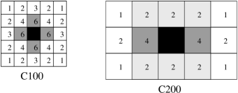
Figure 1: The layout of the rastermaps on the sky. On the left is the C100 layout with a pixel size of $44\arcsec$, on the right is the C200 layout with a pixel size of $92\arcsec$. One square represents one pixel on the sky and the number equals the number of observations of this position. The black square is the source position, observed 9 times with C100 and 4 times with C200. The dark gray squares are used for background determination, for C200 the light gray area is used as average background.

At SRD level only deglitching is performed to correct the remaining cosmic hits or changes in response due to cosmic rays. A sigma of 2.5 is used for the object measurements, and 2.0 for the calibration measurements. The data are processed to Signal per Chopper Plateau (SCP) level by averaging all ramp signals over time per raster point. At SCP level the data are corrected for reset interval and dark current is subtracted. A completely new feature in PIA 8.0 is the correction for a changing response during the measurements, called signal linearization. This is also applied at this level and is a significant improvement in the detection of faint objects, such as ours. After this, only the flux calibration is performed and this introduces the large 30% error in the final flux densities. However, the detection of a source is independent of this calibration and should be assessed separately before the calibration is performed. Thus we use the SCP data to determine the actual S/N for our objects. The noise is calculated from the mean of the errors that PIA gives for the signal on each raster point. The calculation of the signal is difficult, since no pixel average can be used, as the pixels are not corrected for illumination (flatfielded, in optical terms). For each pixel a S/N value is calculated individually and then compared to the median S/N of all pixels. In most cases the deviations are averaged out and the median agrees well with the average S/N for the individual pixels. After the calibration the data are at Astronomical APplication level (AAP) and ready for mapping and background subtraction.

The flux calibration measurements of ISOPHOT are done inside the satellite, using two Fine Calibration Sources (FCS1 and FCS2). For the mini-maps there are two FCS observations of FCS1, one before and one after the source observation. Thus an interpolation is possible to determine the real responsivity at the time of the source measurement. The heating power of the FCS is adjusted to give a signal comparable in strength to the signal expected from the object flux given in the initial observing programme. The observed FCS flux is converted to a real flux using calibration tables constructed with sources for which the flux is well determined. Extrapolation is only possible within a safe range, the so called soft extrapolation limits. Less secure extrapolation is performed up to the hard limits, but outside of these the default responsivities should be used. In our case, all measurements were inside the soft limits and we used the average responsivities from both FCS measurements for all objects.

3.2 ISOPHOT flux determination

Determining the flux density of the sources requires a good method for background subtraction. In our raster maps only the central position is optimally sampled, while the background positions always have less data points available. Fig. 1 illustrates how many data points are available for each sky position and which positions are used for the final source flux density determination.

3.2.1 C100 flux densities

For positions with an oversampling rate of six or more, we calculate the weighted mean of all the pixels that have observed the position. Thus noisy pixels and data taken during the switch-on drift of the detector are excluded almost automatically. Putting all the data points in a spreadsheet provides the possibility to check for other anomalies. In most datasets all pixels are well behaved, but sometimes pixel 5 of the C100 array shows high flux values. This pixel was excluded from the datasets where it was found to bias the final flux density significantly. For the source observations the first pixel to see the source (pixel 7) is excluded, since at this position the detector is severely influenced by the switch-on drift.

Using only the strongly oversampled positions leaves us with four background positions and one source position. In all cases we assume a flat background and match the four observed background flux densities to have no large deviations among them. This involves mainly the exclusion of one or two bad pixels that are either ’hot’ or ’drift’ pixels. In some cases the data are good enough to use all pixels. This method thus provides a possibility to determine a flux without bad pixels and without losing redundancy.

The noise is calculated from the PIA errors given on the signals used in the final flux determination. This means that when bad pixels are excluded, the noise goes down as well. The final value is corrected for PSF.

3.2.2 C200 flux densities

Quasar	160 $\mu$m	90 $\mu$m	60 $\mu$m	galaxy	160 $\mu$m	90 $\mu$m	60 $\mu$m
3C334	7	13	6	3C19	-2	2	0
3C351	14	40	23	3C42	2	3	1
3C323.1	4	4	5	3C460	17	4	0
3C277.1	4	9	4	3C67	4	5	4

Table 2: Signal to noise ratios as determined before the calibration has been applied. See Sect. 3.1 for further details.

The same method is applied as for the C100 data, but with one main difference. Since the redundancy on these data is much lower, only two background values can be calculated. This leaves no possibility to match them, assuming a flat background. Therefore, a third value is calculated using the six positions on either side of the source (see Fig. 1). This value is a good estimate of the background: it excludes any gradients over the source as all positions are distributed symmetrically around the source. The only problem is that the upper three positions are observed by different pixels compared to the lower three, and the flatfield for the C200 array is not very good. Fortunately, most of these errors are averaged out because of the symmetry and the use of weighted means.

3.2.3 PSF corrections

The PSF of both arrays is larger than one pixel. This implies that some of the source flux is in the pixels surrounding the one that observes the source. In the final map this means that the positions around the source see a slightly higher background than the outer positions. Since the PSF is well known for point sources, the correction for this is easy. In PIA 8.0 there is even a flatfield algorithm in the mapping procedure that can correct for this (1st quartile flatfielding) and subsequently the PSF-corrected flux density can be calculated. One should take care in using this however, since this method can create false detections. Therefore, we only use the mapping as a first reference and not to calculate actual flux densities. It is also useful to compare the background fluxes we obtained with the PIA values; they match within 10% for all observations.

3.2.4 Upper limits

The detection of a source is limited by the background flux and the noise on the signal. When a source is placed on a high background, even with low noise on the data it cannot be detected. The same is true for a source on a low background with very noisy data. Thus the calculation of the upper limits should take both the noise on the data and the sensitivity of the detector into account. First the minimum sensitivity of the detectors is calculated for each wavelength separately. This is readily done by dividing the detected fluxes by the background of the same measurement and taking the smallest value. Minimum sensitivities are 3% for C100 and 1% for the C200. This means that on the C100 array a source with only 3/100 of the background flux is still detectable. The efficiency is now defined as the product of the minimum sensitivity and the observed background flux. For each non-detection the efficiency was calculated. This is a first estimate of the flux that can be detected. Then we calculate the noise on the signal, using the same method as described for flux determination. Subsequently, we add 2$\sigma$ noise to the efficiency to obtain an upper limit. Effectively, this corresponds to $\geq 4\sigma$ upper limits for all non-detections.

3.2.5 Calibration error

Due to the large calibration errors for faint sources, the fluxes presented here are to be taken with errors of about 30% (Lemke et al., 1996). These systematical errors are large with respect to the statistical ones and therefore not included in the errors in Fig. 2 and Table 3. The C200 data are taken immediately after the C100 data and thus any calibration errors due to instrumental effects work in the same direction. This implies that the spectral indices are much better determined than the 30% calibration error suggests, and their actual error should be well below 10%.

3.3 VLA and SCUBA data reduction

The VLA data are reduced using standard AIPS routines for mapping and self-calibration. Calibration of the raw interferometer data uses standard VLA flux calibrators and nearby phase calibrators. We do not display the resulting radio maps, as the lack of short spacings prevents reliable imaging of the extended radio lobes. Radio source core flux density values are determined using the MAXFIT procedure. 3C 351 caused some problems during the reduction of its 6 cm and 2 cm observations, due to the strong hot spots in this source. Using the CLEAN procedure with more fields, this problem was solved. In the 6 cm image of the compact 3C 277.1 the core is convolved with the lobe on the western side. Deconvolution with MAXFIT produces a peak flux of around 40 mJy, but since the lobe is not well approximated by a gaussian this value is to be taken as an upper limit. Instead we use the 6 cm literature value (Akujor et al. 1991) of 28 mJy. The quality of the cm data is very high; the errors listed in Table 3 correspond to the 3$\sigma$ noise in the final radio maps. For all sources the errors in the flux density determinations are smaller than the plot symbols in Fig. 2.

The reduction of the 7 mm data appeared to be problematic. The phases change so rapidly in time, that in most cases no solution can be found. The resulting maps then look like noise maps, although a signal can clearly be present when plotting the amplitude $uv$-data in a flux-baseline plot. Only for 3C 277.1 a phase solution is found and a flux density can be determined. In general, for sources below 100 mJy, the 7 mm data appeared impossible to reduce. Thus, the final flux density values may, in theory, range between 0 and 100 mJy. In the case of 3C 334 there is clearly structure in the $uv$ flux-baseline plot, but no phase solution is found. Since it is not possible to determine an upper limit in case of phase fitting errors, we do not include the 7 mm data in the final analysis, except for 3C 277.1.

Object	$F_{6cm}$	$F_{2cm}$	$F_{12mm}$	$F_{7mm}$	$F_{2mm}$	$F_{850\mu}$	$F_{160\mu}$	$F_{90\mu}$	$F_{60\mu}$
3C 334	167.7 $\pm$ 0.8	112.3 $\pm$ 0.4	91.4 $\pm$ 0.7	–	20 $\pm$ 10	15 $\pm$ 8	55 $\pm$ 20	59 $\pm$ 10	86 $\pm$ 22
3C 19	–	–	–	–	–	–	$\leq$65	$\leq$25	$\leq$50
3C 351	9.3 $\pm$ 0.3	5 $\pm$ 1	$\leq$5.0	–	–	–	110 $\pm$ 15	145 $\pm$ 10	211 $\pm$ 23
3C 42	–	–	–	–	–	–	$\leq$45	$\leq$45	$\leq$ 80
3C 323.1	38 $\pm$ 2	43 $\pm$ 1	45 $\pm$ 1	–	$\leq$14	$\leq$12	30 $\pm$ 19	33 $\pm$ 9	49 $\pm$ 18
3C 460	–	–	–	–	–	–	96 $\pm$ 25	14 $\pm$ 7	$\leq$51
3C 277.1	28*	22.7 $\pm$ 0.7	21.5 $\pm$ 1.0	9.6 $\pm$ 1.8	$\leq$17	–	56 $\pm$ 14	30 $\pm$ 10	50 $\pm$ 25
3C 67	–	–	–	–	–	–	73 $\pm$ 50	44 $\pm$ 8	46 $\pm$ 18

Table 3: Flux densities and errors in mJy as plotted in Fig. 2. The value marked with * is from Akujor et al. (1991).

The SCUBA data are reduced using the SCUBA Data Reduction Facility (SURF) and Kernel Application Package (KAPPA). This is a relatively straightforward reduction, since SCUBA is a bolometer array, allowing immediate comparison of the middle bolometer with the surrounding ones. Not all sources were observed at all bands; undetected sources have upper limits, and only 3C 334 has been marginally detected ($\sim 2.5\sigma$) in both bands. The 450 $\mu$m data do not show any source signal, due to the large atmospheric extinction at this wavelength. The upper limits are too high to put any useful constraints on our data and are therefore omitted from Table 3 and Fig. 2. The detections at 850 $\mu$m and 2 mm are marginal at best, but the upper limits provide strong constraints on the non-thermal contamination of the far-infrared emission.

4 Results

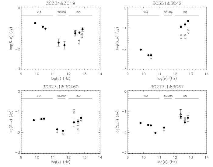
Figure 2: The complete spectra – in their emitted frame – for the four pairs observed with ISO. Filled circles are quasar data, open diamonds are radio galaxy data. The wavelength range of the different instruments is shown in the plots by the horizontal bars.

Since the calibration from detector signal to flux density introduces a substantial error, we make a clear distinction between the detection of a source and the determination of the observed flux. In all cases the detected source has a well determined flux and the objects where the flux measurent is difficult have low S/N. Thus the method is in principle consistent. In practice, however, it is possible that an object is detected but has no flux determination because the calibration errors are too large. In Table 2 we present the S/N values before calibration. We have assumed a detection when the S/N exceeds 3.

In Table 3 we present the resulting flux densities, only with the final 1$\sigma$ intrinsic noise. This value is in general nearly equal to the predicted 30% calibration error. In Fig. 2 we have again plotted only the intrinsic noise, providing better insight into the value of the detection and the spectral indices.

It is clear from Table 3 and Fig. 2 that two pairs exhibit clear flux density differences. In the pair 3C 334 and 3C 19, the radio galaxy is not detected in any band, whereas the quasar has three solid detections (lowest S/N is 6). Since the upper limits take the difference of the backgrounds into account, the radio galaxy is definitely fainter than its paired quasar. In the pair consisting of quasar 3C 351 and radio galaxy 3C 42, the former is unusually bright in the far-infrared (as already observed by IRAS), whereas the radio galaxy has no detections. As the radio core in 3C 351 is relatively weak, the contribution of any beamed non-thermal far-infrared component can be ruled out. The pair consisting of quasar 3C 323.1 and radio galaxy 3C 460 displays a difference at the two short wavelengths. The radio galaxy is not detected at 60 $\mu$m and has a flux density well below that of the quasar at 90 $\mu$m. However, an interesting change occurs at long wavelengths; the 160 $\mu$m flux density of 3C 460 exceeds the 3C 323.1 value. Below we will argue that cool dust associated with star formation is likely responsible for this luminous 160 $\mu$m radiation.

In contrast, the pair consisting of quasar 3C 277.1 and radio galaxy 3C 67 has entirely comparable far-infrared output. Remarkably, this is the pair of Compact Steep Spectrum sources (CSS), objects believed to be young FRIIs where the radio emission is still confined within the host galaxy. Both objects are well detected, with S/N values around 5. Also remarkable in this pair is the high 160 $\mu$m flux for both the radio galaxy and the quasar; the 160 $\mu$m flux densities exceed the 60 $\mu$m values. The only other sample object where this is observed is the radio galaxy 3C 460. It should be noted however, that 3C 67 shows a broad component in H$\alpha$, and hence should be classified as a broad-line radio galaxy. We will return to this issue below.

In all cases the 160 $\mu$m point seems to be higher than what is expected from extrapolating the 90 and 60 $\mu$m data with optically thin grey body models. This could be evidence for cold dust in the host galaxies. Unless contrived colour corrections within the ISOPHOT bands are large and negative, this seems to be a real effect. Because we do not know the intrinsic shape of the spectral energy distribution, we choose not to apply any colour corrections. In general the far-infrared spectra of the quasars indicate a positive spectral index at higher frequencies (i.e., shorter infrared wavelengths) and a flattening towards the lower frequencies. Unfortunately we have no data at mid-infrared wavelengths permitting to determine spectral turnovers in that range, as have been observed in nearby Seyfert galaxies and radio-quiet quasars (Polletta & Courvoisier 1998, Andreani 1998, Klaas et al. 1998). ISO archive data show however that the short wavelength flux densities for 3C 351 are well below our 60 $\mu$m point, implying a peaked spectrum, with the peak somewhere between 60 and 25 $\mu$m.

4.1 Far-infrared luminosities

In order to better compare the observations, we have calculated the luminosities in the ISOPHOT bands: Table 4 lists the resulting values, in Watts. For the spectral index in the K-correction, we used the actual values as observed with ISOPHOT, except for $L_{160}$, where we used $\alpha=0$, assuming that we observe the peak of the cold dust emission with $T\sim 20$ K as observed in normal galaxies (Bianchi et al. 1999) and Seyferts (Rodríguez Espinosa et al. 1996). To make a valid comparison between the radio galaxies and the quasars in the present sample, we calculated the median luminosities at all wavelengths for the different classes. It appears that, with the exception of the CSS pair, the sample quasars are brighter than the radio galaxies at all wavelengths. The median luminosities for the latter always include at least two upper limits, which implies that the actual values for this class are even lower. Thus we can solidly conclude that the quasars are brighter by at least a factor of 1.5 at 60 $\mu$m, which strengthens results from IRAS samples and the Haas et al. (1998) measurements. However, even at longer wavelenghts we find that the median luminosity of the quasars is higher than the median luminosity of the radio galaxies, the latter of which being an upper limit. At 90 $\mu$m the quasars are a factor of 1.5 brighter than the radio galaxies, at 160 $\mu$m this is a factor of 1.3, excluding 3C 460, which is clearly an exceptional object. In summary, the supergalactic size quasars and radio galaxies of our admittedly small ISOPHOT sample differ in their far-infrared output, in the sense that the quasars are brighter than the radio galaxies at all wavelengths by a factor $\sim 1.5$.

4.2 Nature of the infrared emission

Quasar	log($L_{160}$)	log($L_{90}$)	log($L_{60}$)	Galaxy	log($L_{160}$)	log($L_{90}$)	log($L_{60}$)
3C334	37.68	38.00	38.11	3C19	$\leq$37.64	$\leq$37.65	$\leq$37.75
3C351	37.64	38.00	38.16	3C42	$\leq$37.33	$\leq$37.72	$\leq$37.86
3C323.1	36.82	37.22	37.35	3C460	37.34	37.12	$\leq$37.37
3C277.1	37.25	37.44	37.47	3C67	37.34	37.49	37.51
Median QSR	37.45	37.72	37.79	Median RG	$\leq$37.34	$\leq$37.57	$\leq$37.63

Table 4: Luminosities ($log(\nu L_{\nu})$)calculated from the ISO observations, units are in W. The spectral indices are calculated from the observations, while for non-detections we have used the extreme value, to obtain an upper limit for the luminosity. For the L₁₆₀ we used $\alpha$=0. We adopt $F_{\nu}\propto\nu^{\alpha}$.

From Fig. 2 it is clear that the extrapolation of the radio core spectrum to the infrared underpredicts the observed infrared flux densities. This implies that (relativistically beamed) nonthermal radiation is not contributing significantly in the present quasars. The only exception could be 3C 334, where a maximum of about 10% beamed radiation might be present in the infrared, confirming previous results (van Bemmel et al. 1998). Still, this is not enough to explain the difference between 3C 19 and 3C 334, given that their flux densities appear to differ by about a factor of two. The contribution of beamed non-thermal emission is well below 2% in the other cases. This implies that the bulk of the observed far-infrared emission in the sample objects must be of thermal origin.

4.3 Dust mass estimates

Having established the thermal origin of the infrared emission, we can estimate the dust mass responsible for the radiation. Because the high 160 $\mu$m points render a single component grey body fit impossible, we fitted the observations with a two temperature grey body. Since this requires a four component fit to three points, we kept the temperatures constant throughout the sample to obtain a uniform estimate of the dust masses. The temperatures are chosen to be 75 K for the warm component, as we are not sensitive to much higher temperatures due to the limited wavelength coverage, and 20 K for the cold component (as observed from cold cirrus in nearby galaxies, Bianchi et al. 1999, Rodríguez Espinosa et al. 1996). Only for 3C 460 did the fit require a slightly lower temperature for the cold component of 18 K. Calculating the dust masses with fixed temperatures gives an average mass of $3\times 10^{5}$ $M_{\odot}$ for the warm component and $1.5\times 10^{8}$ $M_{\odot}$ for the cold one.

5 Discussion

With the absolute flux uncertainties of ISOPHOT and the small sample under study, we are not able to constrain the model predictions from either the unification theory or the dust models for Seyfert galaxies. Any statistical analysis will be severly biased by the individual characteristics of the objects in the sample. We therefore choose to only compare the median luminosities of the two classes. Below we discuss shortcomings of the present samples as well as various alternative interpretations of the ISOPHOT data.

5.1 Compact versus extended sources

The pair containing subgalactic size CSS sources stands out; they have (within the errors) identical infrared output. While this could – most interestingly – be a general property of dust emission from the host galaxies of young radio sources, it could also relate to the fact that we have matched a broad-line radio galaxy to a quasar. 3C 67 has been reported to have broad H$\alpha$ (Eracleous & Halpern 1994), but is otherwise in its spectral characteristics clearly different from strong quasars such as 3C 277.1. It will be interesting to examine the ISO archive in order to see if the compact sources in general have comparable infrared output, whether classified as quasar or radio galaxy, or if we have made a mismatch in this case.

5.2 Size and AGN luminosity differences

Inspection of Table 1 shows that although the observed paired objects match in redshift and radio luminosity, they differ in projected linear radio size, the quasars being signifantly larger (with the exception of the CSS pair). Within the framework of the unification model, the size difference would be even more pronounced, given the larger deprojection factor for the quasars. This fact, although purely coincidental, might have severe consequences for the interpretation of our results. On the basis of model evolutionary tracks in the P–D diagrams (e.g. Kaiser et al. 1997), larger objects with the same radio power should have more powerful jets. Within this scenario, the AGN strengths, and consequently the far-infrared output of our sample quasars, could be at least a factor of two larger as compared to the radio galaxies, which matches our observations.

In addition, within the so-called receding torus model and given the possibility of some scatter in the optical-UV AGN luminosity, the average quasar may be a factor $\sim$2 more luminous than the average radio galaxy, when drawn from a sample having one and the same radio luminosity (Simpson 1998).

Along these lines, we may have paired powerful quasars with somewhat less powerful radio galaxies. This explanation could in principle be tested by intercomparison of the luminosities in the [OIII] and/or [OII] emission lines, arising in the circumnuclear narrow-line region. While not enough [OII]$\lambda 3727$ data are available in the literature, the [OIII]$\lambda\lambda$4959,5007 line luminosity will be inconclusive, as the latter is known to be anisotropic (Hes et al. 1996), due to dust extinction within the narrow line region (di Serego Alighieri et al. 1997, Baker 1997).

Analysis of the FIR properties of much larger samples, covering larger parameter space will be needed to address these effects.

5.3 Host galaxy contribution

Strong evidence for a host galaxy contribution comes from 3C 460, where a cold dust mass of 2.4$\times 10^{8}$ M_⊙ is observed. This amount of dust is most likely due to star formation in the host galaxy, which could be related to a close companion galaxy at 1.5$\arcsec$ separation (de Koff et al. 1996). A distinction between torus, starburst and cold cirrus dust was already made by Rowan-Robinson (1995). From 60$\mu$m data on PG quasars there is indeed evidence that this emission is at least in part produced by star formation (Clements, 2000). Thus dust in the host galaxy can dilute the emission from a (warmer) dust torus.

5.4 Variability of the non-thermal component

Non-thermal flares which can occur within days have been observed in blazars, and should be observable in all AGN with a jet-axis close to the line of sight. These flares peak in the millimeter range (Brown et al. 1989), and can be responsible for strong variability down to far-infrared wavelengths. We do not cover the spectral range where these flares are observed, nor do we have the time resolution to detect any variability. Thus variability cannot be excluded by our data.

5.5 Anisotropy in the torus emission

All models for emission from a dust torus heated by a central AGN are based on parameters deduced from Seyfert galaxies. A straightforward application to the stronger radio galaxies and quasars might not be possible, as these sources have generally much stronger central cores and different hosts. Their tori might be much thicker and denser and thus emit optically thick at the observed wavelengths.

6 Conclusions

Observations of pairs of radio-loud quasars and radio galaxies confirm the previously reported far-infrared excess in quasars and indicate that this excess extends up to restframe wavelengths of $\sim 130\,\mu$m. However, the origin of this excess remains unclear and may lie in the biases introduced in our limited sample. It has been shown that more than 98% of the observed far-infrared emission is of thermal origin, with the exception of 3C 334, where non-thermal emission might contribute up to 10%. The 160 $\mu$m data points are always higher than the expected flux densities for grey body emission, which suggests the presence of a cold component in all objects. In 3C 460 we report the discovery of a comparatively large cold dust content, which could be related to interaction with a close companion.

In order to explain the observed difference in infrared output, we discuss several possibilities, such as size difference, host contributions, non-thermal flares, anisotropy of the torus, and a true AGN power difference. With the present quality and limited amount of data we are not able to discriminate between either of these. We stress the need for better modelling of torus emission for 3C-like objects, which is at present not available for the wavelengths under consideration. Further analysis of ISOPHOT data on similar objects will be undertaken to enlarge the sample and better constrain the models.

- (1) Akujor C.E., Spencer R.E., Zhang F.J., et al., 1991, MNRAS 250, 215
- (2) Andreani P., 1998, in ’The universe as seen by ISO’, 20 – 23 October 1998, Paris, ESA SP-427, p.857
- (3) Antonucci R., 1993, ARA&A 31, 473
- (4) Baker J. C., 1997, MNRAS 286, 23
- (5) Barthel P.D., 1989, ApJ 336, 606
- (6) Bianchi S., Alton P.B., Davies J.I., 1999, in ’ISO beyond point sources’, 14 – 17 September, 1999, VILSPA
- (7) Bogers W.J., Hes R., Barthel P.D., Zensus J.A., 1994, AAS 105, 91
- (8) Bridle A.H., Hough D.H., Lonsdale C.J., et al., 1994, AJ 108, 766
- (9) Brown L.M.J., Robson E.I., Gear W.K., et al., 1989, ApJ 340, 129
- (10) Clements D.L., 2000, MNRAS 311, 833
- (11) de Koff S., Baum S.A., Sparks W.B., et al., 1996, ApJS 107, 621
- (12) de Vries W.H., O’Dea C.P., Baum S.A., et al., 1998, ApJ 503, 156
- (13) di Serego Alighieri S., Cimatti A., Fosbury R.A.E., Hes R., 1997, A&A 328, 510
- (14) Eracleous M., Halpern J.P., 1994 ApJS 90, 1
- (15) Fanaroff B.L., Riley J.M., 1974, MNRAS 167, 31P
- (16) Fanti R., Fanti C., Schilizzi R.T., et al., 1990, A&A 231, 333
- (17) Fernini I., Burns J.O., Perley R.A., 1997, AJ 114, 2292
- (18) Granato G.L., Danese L., 1994, MNRAS 268, 235
- (19) Haas M., Chini R., Meisenheimer K., et al., 1998, ApJ 503, L109
- (20) Heckman T.M., O’Dea C.P., Baum S.A., Laurikainen E., 1994, ApJ 428, 65
- (21) Hes R., Barthel P.D., Hoekstra H., 1995, A&A 303, 8
- (22) Hes R., Barthel P.D., Fosbury R.A.E., 1996, A&A 313, 423
- (23) Hoekstra H., Barthel P.D., Hes R., 1997, A&A 319, 757
- (24) Impey C.D., Neugebauer G., 1988, AJ 95, 307
- (25) Jenkins C.R., Pooley G.G., Riley J.M., 1977, MemRAS 84, 61
- (26) Kaiser C.R., Dennett-Thorpe J., Alexander P., 1997, MNRAS 292, 723
- (27) Klaas U., Haas M., Schulz B., 1998, in ’The universe as seen by ISO’, 20 – 23 October 1998, Paris, ESA SP-427, p.901
- (28) Laing R.A., 1980, MNRAS 193, 439
- (29) Lemke D., Klaas U., Abolins J., et al., 1996, A&A 315, L64
- (30) Ogle P.M., Cohen M.H., Miller J.S., et al., 1997, ApJ 482, L37
- (31) Pier E.A., Krolik J.H., 1992, ApJ 401, 99
- (32) Polletta M., Courvoisier T.J.-L., 1998, in ’The universe as seen by ISO’, 20 – 23 October 1998, Paris, ESA SP-427, p.953
- (33) Rawlings S., Saunders R., 1991, Nat. 349, 138
- (34) Rodríguez Espinosa J.M., Pérez García A.M., Lemke D., Meisenheimer K., 1996, A&A 315, L129
- (35) Rowan-Robinson M., 1995, MNRAS 272, 737
- (36) Sanghera H.S., Saikia D.J., Lüdke E., et al., 1995, A&A 295, 629
- (37) Simpson C., 1998, MNRAS 297, L39
- (38) Stockton A., Ridgway S.E., 1991, AJ 102, 488
- (39) Tadhunter C.N., Packham C., Axon D.J., et al., 1999, ApJ 512, L91
- (40) Ueno S., Koyama K., Nishida M., Yamauchi S., Ward M., 1994, ApJ 431, L1
- (41) Urry C.M., Padovani P., 1995, PASP 107, 803
- (42) van Bemmel I.M., Barthel P.D., Yun M.S., 1998, A&A 334, 799
- (43) Willott C.J., Rawlings S., Blundell K.M., Lacy M., 1999 MNRAS 309, 1017
- (44) Wink J.E., Guilloteau S., Wilson T.L., 1997, A&A 322, 427