Voids in the LCRS versus CDM Models

Abstract

We have analyzed the distribution of void sizes in the two-dimensional slices of the Las Campanas Redshift Survey (LCRS). Fourteen volume-limited subsamples were extracted from the six slices to cover a large part of the survey and to test the robustness of the results against cosmic variance. Thirteen samples were randomly culled to produce homogeneously selected samples. We then studied the relationship between the cumulative area covered by voids and the void size as a property of the void hierarchy. We find that the distribution of void sizes scales with the mean galaxy separation, $\lambda$. In particular, we find that the size of voids covering half of the area is given by $D_{med}\approx\lambda+(12\pm 3)\,h^{-1}{\mbox{Mpc}}$. Next, by employing an environmental density threshold criterion to identify mock galaxies, we were able to extend this analysis to mock samples from dynamical $n$-body simulations of Cold Dark Matter (CDM) models. To reproduce the observed void statistics, overdensity thresholds of $\delta_{th}\approx 0\dots 1$ are necessary. We have compared standard (SCDM), open (OCDM), vacuum energy dominated ($\Lambda$CDM), and broken scale invariant CDM models (BCDM): we find that both the void coverage distribution and the two-point correlation function provide important and complementary information on the large-scale matter distribution. The dependence of the void statistics on the threshold criterion for the mock galaxy indentification shows that the galaxy biasing is more crucial for the void size distribution than are differences between the cosmological models.

1 Introduction

Voids in the distribution of galaxies were first noticed in early studies of the large scale distribution of galaxies, Jõeveer et al. (1978), Gregory & Thompson (1978), Tully & Fisher (1978), Chincarini & Rood (1979), and Tarenghi et al. (1979). The void behind the Perseus-Pisces supercluster (Jõeveer et al. (1978)) and the Boötes void (Kirshner et al. (1981)) both have diameters of about 70 $h^{-1}$Mpc ($H_{0}=100~{}h~{}$km s^-1 Mpc^-1). The presence of voids was explained by Einasto, Jõeveer & Saar (1980) and Zel’dovich, Einasto & Shandarin (1982) by gravitational instability. Matter disperses by outflow from low-density regions (voids), and the rest remains there in primordial form; in high-density regions, however, the matter collapses and forms superclusters, filaments of galaxies, and clusters. The resulting picture resembles a ‘cellular’ structure and is well described by the pancake theory of Zel’dovich (1970). The evacuation of matter in voids has been traced back to the underlying large-scale potential distribution by Coles, Melott & Shandarin (1993), Lee & Shandarin (1998), and Madsen et al. (1998). The galaxy distribution has also been characterized either as a ‘foam’ of bubbles (de Lapparent, Geller & Huchra (1986)) or as a ‘sponge-like network’ of interlocking filaments and tunnels connecting overdense and empty regions (Gott, Melott & Dickinson (1986)). More recent studies have shown that voids may be populated and subdivided into smaller voids by fainter galaxies, cp. Lindner et al. (1995) and Popescu, Hopp & Elsässer (1997). Observationally, there is no doubt that large underdense regions which contain almost no galaxies are a common feature of the large scale structure. Furthermore, numerical simulations demonstrate that filaments and voids form in a hierarchy of scales for any physically reasonable model of structure formation (Melott et al. (1983)).

In the past, properties of voids have been characterized by the void probability function (White (1979)) and by the statistics of void diameters (Einasto, Einasto & Gramann (1989)). The void probability function has a clear statistical interpretation; however, it falls off quickly below 20 $h^{-1}$Mpc as seen in the CfA catalog by Vogeley, Geller & Huchra (1991), in the 1.2 Jy IRAS survey by Bouchet et al. (1993), and in the SSRS by da Costa et al. (1994). Therefore, it is not very sensitive to the matter distribution on large scales. On the other hand, the distribution of diameters of maximum voids describes better the distribution of galaxies and clusters on large scales. Numerical simulations within CDM models (Einasto et al. (1991), Little & Weinberg (1994), Jing et al. (1994), Vogeley et al. (1994), Ghigna et al. (1994), and Ghigna et al. (1996)) have shown that CDM models can explain the observed void probability function for a suitable cosmological model and a corresponding bias model. Appropriate models can also reproduce the dependence of the void sizes on the mean galaxy density in the catalogues.

So far, void statistics have been investigated using galaxy surveys which cover a large area on the sky. Up till now, the deepest surveys employed in such analysis have had radial extents of about 150 $h^{-1}$Mpc. For this reason, the measured size of voids was mostly restricted by the size of the survey volume. That is, until now, there has never been a statistically complete measurement of the void distribution; previous measurements have all been truncated at the high end by the survey depths. The aim of this paper is to study void properties in the Las Campanas Redshift Survey (LCRS), which has a depth of about 600 $h^{-1}$Mpc ($z\mathrel{\hbox to0.0pt{\lower 3.0pt\hbox{$\mathchar 536\relax$}\hss}\raise 2.0pt\hbox{$\mathchar 316\relax$}}0.2$). This depth is large enough to contain a sufficient number of voids for a statistical analysis; thus this sample is better suited for the investigation of void properties over a broader scale interval. The price to be paid is that the survey consists of 6 narrow strips on the sky, i.e. it is effectively 2-dimensional. We take this into account and project the galaxies on the six central planes, and we perform a void analysis in two dimensions. To this aim, we apply the void finder algorithm developed by Kauffmann & Fairall (1991) and Kauffmann & Melott (1992) (similar algorithms can be found in El-Ad & Piran (1997), El-Ad, Piran & da Costa (1997), and El-Ad & Piran (2000)). The void finder puts arbitrarily formed but approximately convex voids of maximal size into the galaxy distribution. Then we study the mean fractional area covered by voids (Kauffmann & Melott (1992)), as it is a stable characteristic of the void distribution. We also compare the properties of voids in the LCRS with voids in large simulations of CDM models with different cosmological parameters.

The paper is organized as follows. In Section 2 we describe the selection of volume limited samples from the different slices of the LCRS and analyze the distribution of void sizes in the selected data sets. In Section 3 we present results of numerical simulations of four cosmological models, discuss the prescription for establishing mock catalogues, and apply the void finder to them. In section 4 we compare data and simulations and draw our conclusions.

2 Voids in volume limited subsamples of the LCRS

The LCRS is the deepest redshift survey presently available (Shectman et al. (1996)). The survey contains 24,518 galaxy redshifts in 3 slices in the northern and in 3 slices in the southern galactic hemisphere. Each slice extends $\approx 80^{\circ}$ in right ascension and $\approx 1.5^{\circ}$ in declination. The northern galactic hemisphere slices are centered at $\delta=-3^{\circ},-6^{\circ},-12^{\circ}$, and the southern at $\delta=-39^{\circ},-42^{\circ},-45^{\circ}$. Here, we select volume limited subsamples in the different slices, correct for the non-uniform sampling rate, and project the galaxies to the central plane. Taking into account the dominant two-dimensional geometry of the LCRS, we look for two-dimensional voids in these planes. Whether these voids are representative for voids in the three-dimensional galaxy distribution will be discussed in a future paper.

Figure 1: Selection of the volume limited subsamples 7, 8, and 9 in the $\delta=-12^{\circ}$ slice. The magnitude limits of $m_{R}=15$ and 17.7 and of $m_{R}=16$ and 17.3 for the high and low sampling rate are shown as solid and dashed curves, respectively.

2.1 Selection of volume limited subsets

The LCRS contains galaxies within apparent magnitude ranges of $16<m_{R}<17.3$ and of $15<m_{R}<17.7$ for the 50 and 112-fiber fields, respectively. Therefore we must impose both lower and upper limits in depth and absolute magnitude to define volume limited samples. We select lower and upper limits of the luminosity distances, $d_{1}$ and $d_{2}$, respectively, which cover the well sampled region of the survey (see, for instance, Fig. 1). For determining luminosity distances $d$, we employ the relation of Mattig (1958) with $q_{0}=0.2$ and a $k$-correction $k(z)=2.5\log(1+z)$, which is representative for the galaxy mix in the LCRS (Lin et al. (1996)). From the distance limits and the apparent magnitude range of the survey, we get lower and upper limits of the absolute magnitude $M>M_{1}$ and $M<M_{2}$, within which galaxies are observed in the chosen distance range (Fig. 1). In all slices we select at least 2 absolute magnitude limited samples in different magnitude ranges in order to test our results for a possible dependence on absolute magnitude. The corresponding limits for 14 data sets are listed in Table  1.

Each slice in the LCRS consists of a collection of $1.5\deg^{2}$ fields with different sampling characteristics which depend both on the instrument used to obtain the spectra (either a 50-fiber or a 112-fiber spectrograph) and on the local galaxy surface density within that field. Therefore, there are field-to-field sampling variations within each slice. To obtain homogeneously sampled slices, we randomly dilute the higher sampled fields to the minimum sampling rate in the corresponding slice, as is shown in the third column of Table 1. Only in the final set 14 of Table 1 do we keep all the galaxies. We take this set as control sample to have both a high galaxy number and a high surface density. This set is used to test the effects of random sampling. The resulting galaxy numbers are given in the 8th column; these vary strongly due to the different magnitude ranges and sampling fractions. Column 9 shows the mean galaxy separation $\lambda=\sigma^{-1/2}$, where $\sigma$ is the surface density of galaxies. There are large differences in the galaxy density and in the volume covered by the different data sets. In particular, sets 7 and 8, which stem from the one slice which was observed entirely with the 112-fiber spectrograph, have a high galaxy density and are expected to give statistically reliable results. We employ the dependence of the void statistics on the galaxy density in our further analysis. It should be remarked that we keep the galaxy slices in a wedge-like geometry. A similar geometry is taken for the study of the mock samples, and we discuss the effect of the geometry and of boundary effects below.

Table 1: Properties of the volume limited subsamples of LCRS

set	slice	$f_{min}$	$M_{1}$	$M_{2}$	$d_{1}$	$d_{2}$	$N_{gal}$	$\lambda$	$D_{med}$	$D_{max}$
					$h^{-1}$Mpc	$h^{-1}$Mpc		$h^{-1}$Mpc	$h^{-1}$Mpc	$h^{-1}$Mpc
1	-45	.21	-20.20	-21.10	220	320	138	12.56	31.2	38.4
2	-45	.21	-21.00	-21.80	320	440	136	15.83	29.6	53.6
3	-42	.28	-20.30	-20.80	210	330	182	14.26	27.2	40.8
4	-42	.28	-20.90	-21.60	300	420	165	16.52	32.8	47.2
5	-39	.30	-20.50	-21.00	235	360	221	14.08	28.8	55.2
6	-39	.30	-20.90	-21.40	280	420	182	17.43	29.6	55.2
7	-12	.45	-19.95	-21.35	175	325	829	7.05	20.0	40.8
8	-12	.45	-20.40	-21.65	200	400	803	8.85	21.6	44.0
9	-12	.45	-20.90	-22.20	250	500	638	12.04	27.2	46.4
10	-6	.39	-20.10	-20.70	200	300	223	10.96	20.8	38.4
11	-6	.39	-20.60	-21.40	280	380	213	12.47	21.6	37.6
12	-3	.37	-20.00	-20.40	180	280	174	12.27	24.0	38.4
13	-3	.37	-20.50	-21.10	240	360	280	11.79	22.4	42.4
14	-12	–	-20.40	-21.65	200	400	1217	7.25	21.6	37.6

2.2 Void statistics in the LCRS

Figure 2: Large voids with extensions in set 7 selected from the $\delta=-12^{\circ}$ slice. Points represent the projected galaxy positions and the point size is proportional to the galaxy’s absolute magnitude.

As illustrated in Fig. 2, we employ the algorithm of Kauffmann & Fairall (1991) to define voids in a two-dimensional plane of the LCRS. To this aim we construct a density field on a rectangular $1000\times 1000$ grid covering the survey plane, placed into a square of 800 $h^{-1}$Mpc on a side. The density field is defined by the galaxy number per cell, and voids are connected samples of empty cells. The algorithm places maximal square boxes into the galaxy distribution. As a next step, extensions to each base void are constructed along all sides with the restriction that each extension is a connected row of empty cells with length exceeding two-thirds of the previous extension (or the base of the square void). This provides a good approximation of convex voids as illustrated in Fig. 2. In particular, it avoids the situation of single voids consisting of different convex regions connected by narrow tunnels. After defining a void, the void cells are marked, and voids with smaller base sizes are determined in the rest of the plane. Unlike other algorithms, such as smoothing the density field and fitting ellipsoids into underdense regions, we make no additional assumptions about the void shape besides near convexity. The void finder which we have applied looks for completely empty regions in the galaxy distribution. Possibly this restriction may be circumvented in a further development of the algorithm.

Of special importance for the void statistics is the treatment of the boundary of the data sets. After some trial and error, we decided to count all cells outside of the survey region as occupied. That means that no voids are allowed to enter the boundary of the survey (see Fig. 2). This will restrict the size of some voids near the boundary, and thus shift the void distribution slightly to smaller sizes $D$. Tests with mock galaxy samples in larger volumes and in the survey geometry show that this underestimation is less than 3%. We employ similar geometries both in the observed data and in the mock samples in order to be independent of this underestimation. Nonetheless, the effect should be taken into account in the quantitative evaluation of the void sizes.

Here we look for the size distribution of voids, where the size is measured by the length $D$ of the base voids. We measure the abundance of voids by the fraction of the slice area which is covered by voids of a given size. In Fig. 3 we show the cumulative distribution of the coverage of the planes of the LCRS data sets. The smoothness of the histograms illustrates both the good statistics which we get with our 14 data sets and the large depth of the LCRS. The void distributions have obviously a similar shape. The different curves show that larger void sizes are typical for data sets with larger mean galaxy separation $\lambda$ as given in Table 1. A scaling of the void sizes with the galaxy density was already noticed by Ryden & Turner (1984) who found that the maximum void size $D_{max}$ (with their void definition)

$$D_{max}\approx(2-3)n^{-1/3}.$$ (1)

For our two-dimensional data this corresponds to a scaling $\propto\lambda=\sigma^{-1/2}$, which will be used in the following analysis. Here we show the real physical sizes to demonstrate that voids of (20 - 40) $h^{-1}$Mpc base sizes are typical for the bright galaxies sampled in the LCRS. Some voids have a size of up to 55 $h^{-1}$Mpc. They are rare, however, and their statistics are noisy.

Figure 3: Cumulative distribution of the fraction $f$ of the LCRS slices covered by voids of size $D$. The solid lines show the better sampled sets 7, 14, 8, 10, 13, 12, 1, 9, 11 (from left to right) with $\lambda\mathrel{\hbox to0.0pt{\lower 3.0pt\hbox{$\mathchar 536\relax$}\hss}\raise 2.0pt\hbox{$\mathchar 316\relax$}}12$ $h^{-1}$Mpc; the distributions for the other sets are dotted.

The basic factor that determines the void size distribution is the mean galaxy surface density, $\sigma$, or, equivalently, the mean galaxy separation $\lambda=\sigma^{-1/2}$. We show in the last two columns of Table 1 the median and the maximum void size, $D_{med}$ and $D_{max}$, respectively. In Fig. 4, we show the $\lambda$ dependence of the median and quartile values of the void sizes – i.e. those values that lead to a 25% , 50%, and 75% coverage of the survey area if the void areas are added starting from small sizes. These values show the expected dependence on the galaxy separation $\lambda$,

$$D\approx\nu\lambda+D_{0},$$ (2)

with a residual void size $D_{0}$ for ‘zero mean separation’ and a slope $\nu$ for the size increase if a random subset of the data is studied. The residual value $D_{0}$ is a somewhat formal quantity since the minimum mean separation for bright galaxies as sampled in the LCRS amounts a few Mpc. Furthermore, $D_{0}$ is not well determined since it lies well outside of the $\lambda$ range of the fit ($7<\lambda<17.5\,h^{-1}{\mbox{Mpc}}$); note the quite large uncertainty of this value for the data in Table 2, in which the values for the typical void sizes and the slopes $\nu$ are tabulated. The 1-$\sigma$ errors in the parameter ranges originate from the different data sets, i.e. they include statistical effects from different parts of the survey, from possible systematic effects in the void finder as using the wedge geometry, boundary effects, and also systematic effects due to different volumes and magnitudes in the different data sets. The last systematics is more intensely discussed below. It can be noted that a Poisson sample leads typically to a slope $\nu\approx 2$ and to a residual value $D_{0}$ consistent with zero, i.e. not unexpectedly, it is strongly different from the void statistic of the LCRS data.

A similar relation for the mean void size of a Poisson sample of points in 3 dimensions, $D_{med}\approx 3\lambda$, was given in Lindner et al. (1995). The relation for the maximum void size in Eq. (1) from Ryden & Turner (1984) corresponds to $\nu\approx 2-3$ and no residual value, which is typical for a Poisson point distribution. Obviously, a quite undersampled data set was used in their analysis. Our relation in Eq. (2) seems more typical for the void size distribution in a clustered galaxy distribution, and an indication on a residual value is also seen in the void distribution of Lindner et al. (1995) (see Fig. 9 in their paper, where the relation of the void size and the galaxy number is shown). The residual median void size, $D_{0}\approx 12\,h^{-1}{\mbox{Mpc}}$, is taken as a typical size of voids in well sampled parts of the LCRS. It substantially exceeds the corresponding values for the Poisson samples given in the second row of Table 2. Also, the slope of the fractional increase of the void size for diluted samples, $\nu\approx 1$, is significantly different from that for the Poisson samples, $\nu\approx 2$. Obviously, the void sizes grow much more quickly in diluted data sets for the random samples than for the clustered data, and $\nu\approx 1$ is a typical result that must be reproduced by simulated data sets. It is also remarkable that the inhomogeneous data set 14 lies on the same fit. This means that some inhomogeneity in the galaxy sampling does not destroy the typical distribution of observed voids.

There are no major differences between the void distributions for different bright galaxy samples, as the comparison of the void statistics of data sets 1 and 12 with the much brighter data sets 9, 11, and 13 demonstrates (see Fig. 5 and Table 1). Their median sizes show no strong trend with the magnitude range, and only the maximum void size of set 9 exceeds all the others due to its larger volume. We do not regard the maximum void size as a reliable statistics for our comparison of data and simulations. In Fig. 5 we show the median void sizes of the 14 data sets versus the lower limit of the absolute magnitude range $M_{1}$. There is a trend of increasing void sizes for more luminous galaxies. However, this trend is masked by differences in the dilution factor, as seen by comparison of the data sets sampled with high ($f_{min}>0.35$) and low ($f_{min}<0.35$) sampling rate. Thus we shall use in the following analysis the mean galaxy separation in different data sets as the argument which determines void sizes. We studied Pearson’s linear correlation $r$ (see, e.g. Press, et al. (1992)) of the median void size $D_{med}$ and the mean galaxy separation $\lambda$, which is $r=0.81$ with error probability 0.04%. This indicates a clear correlation with high reliability. Taking the dependence of the median void size $D_{med}$ on the lower absolute magnitude limit $M_{1}$ and the sampling fraction $f_{min}$, we get much weaker correlation coefficients of $r=0.57$ and $r=0.56$, with 3% and 4% error probability, respectively. Hence, basically, the first dependence, $D_{med}$ on $\lambda$, shows a tight correlation. This formal test shows that for the restricted range of $M_{1}$ which could be tested with the given data the dependence of void sizes on the absolute magnitude limit cannot be established reliably.

An other important effect which plays a role is the wedge-like geometry of the LCRS data sets – i.e, the LCRS slices are not rectangular volumes, but wedges with an opening angle of $1.5^{\circ}$. This leads to a slight density gradient over the survey plane and – as shown by the scaling in Eq. (2) – to somewhat smaller voids in the more distant parts of the survey planes and to somewhat larger voids in the less dense sampled parts of the nearby regions. The addition of small voids concerns less than half of the volume, whereas small voids are less abundant in the other part due to the large volume occupied by the big voids. Tests with simulations show that the cumulative void distribution in Fig. 3 is shifted to larger void sizes $D$ by $(5-10)\%$. This overestimate of void sizes also affects all mean characteristics of the void distribution that are shown in Fig. 4 and given in Table 2. The same effect occurs in the mock samples; i.e., this effect does not influence the comparison of the data with models. Tests have shown that it is more reliable to keep a higher galaxy number in the volume limited samples rather than to reduce further the galaxy number in order to get samples with constant thickness. Finally, we remarked above that the boundary effects of the survey tend to slightly reduce the typical void size – i.e., they yield a competing effect to that of the slices’ wedge-like geometry. Even so, as mentioned above, this competing influence is smaller (only $\approx 3\%$).

Table 2: Void distribution in data and mock samples for some CDM models: model parameter and fits to the residual void size $D_{0}$ and and slope $\nu$ of void size increase.

sets	$\Omega_{m}$	$h$	$\sigma_{8}$	$\delta_{th}$	$\delta_{cr}$	median		lower quartile		upper quartile
						$D_{0}$	$\nu$	$D_{0}$	$\nu$	$D_{0}$	$\nu$
						$h^{-1}$Mpc		$h^{-1}$Mpc		$h^{-1}$Mpc
data						$11.8\pm 2.9$	$1.1\pm 0.2$	$5.7\pm 1.6$	$0.9\pm 0.1$	$16.8\pm 2.9$	$1.5\pm 0.2$
Poisson						$0.9\pm 1.0$	$1.8\pm 0.1$	$0.9\pm 0.3$	$1.2\pm 0.1$	$2.1\pm 0.5$	$2.1\pm 0.1$
SCDM mock1	1	0.5	1.3	-0.9	400	$5.7\pm 1.2$	$1.6\pm 0.1$	$1.6\pm 0.7$	$1.0\pm 0.1$	$6.8\pm 1.2$	$2.2\pm 0.1$
SCDM mock2	1	0.5	1.3	0	250	$9.6\pm 1.1$	$1.2\pm 0.1$	$1.3\pm 0.8$	$1.2\pm 0.1$	$14.6\pm 1.1$	$1.4\pm 1.1$
SCDMc mock3	1	0.5	0.6	0.2	900	$5.1\pm 1.2$	$1.5\pm 0.1$	$1.0\pm 1.5$	$1.1\pm 0.1$	$11.9\pm 1.2$	$1.4\pm 0.1$
$\Lambda$CDM mock4	0.3	0.65	1.2	-0.9	600	$4.1\pm 0.9$	$1.9\pm 0.1$	$1.2\pm 0.9$	$1.2\pm 0.1$	$8.6\pm 1.5$	$2.2\pm 0.1$
$\Lambda$CDM mock5	0.3	0.65	1.2	-0.5	300	$6.3\pm 1.5$	$1.8\pm 0.1$	$1.6\pm 1.7$	$1.2\pm 0.2$	$11.9\pm 1.7$	$2.0\pm 0.1$
$\Lambda$CDM mock6	0.3	0.65	1.2	0	200	$5.8\pm 1.5$	$1.9\pm 0.1$	$2.7\pm 0.6$	$1.1\pm 0.1$	$17.8\pm 1.0$	$1.5\pm 0.1$
$\Lambda$CDM mock7	0.3	0.65	1.2	1	100	$7.6\pm 0.9$	$1.5\pm 0.1$	$2.9\pm 1.2$	$1.1\pm 0.1$	$14.2\pm 1.2$	$1.8\pm 0.1$
OCDM mock8	0.5	0.6	0.9	0	4000	$6.6\pm 0.5$	$1.5\pm 0.1$	$2.5\pm 0.4$	$1.1\pm.03$	$10.4\pm 0.9$	$2.0\pm 0.1$
OCDM mock9	0.5	0.6	0.9	1	500	$5.2\pm 1.4$	$1.7\pm 0.1$	$4.5\pm 0.9$	$1.0\pm 0.1$	$5.9\pm 0.9$	$2.4\pm 0.2$
OCDM mock10	0.5	0.6	0.9	2	300	$10.7\pm 1.8$	$1.2\pm 0.2$	$4.8\pm 0.6$	$1.0\pm 0.1$	$15.7\pm 2.7$	$1.8\pm 0.2$
BCDM mock11	1	0.5	0.6	0.5	20000	$7.7\pm 0.9$	$1.5\pm 0.1$	$1.8\pm 1.0$	$1.2\pm 0.1$	$10.2\pm 3.6$	$2.3\pm 0.4$

Figure 4: Median (squares) and quartile (diamonds) values of the void sizes in the LCRS versus the mean galaxy separation $\lambda$ in the 14 volume limited data sets. The straight lines give the linear fits of Eq. (2) to the data. The small circles (filled for median and open for quartiles) show the corresponding void sizes in the mock sample 8 of the OCDM simulation (which has typically too small void sizes for small $\lambda$).

Figure 5: Median values of the void sizes in the LCRS versus the lower absolute magnitude limit $M_{1}$ in the 14 volume limited data sets. The filled symbols show data sets with a sampling rate $f_{min}>0.35$, the open symbols less well sampled data with $f_{min}<0.35$. The numbers at the symbols show the different data sets from Table 1.

3 Voids in CDM mock samples

For evaluation of our results we compare them with a set of numerical simulations and corresponding mock samples of model galaxy distributions in different CDM models. We compare the model galaxy distribution also with the 2-point correlation function of galaxies with a similar range in brightness as that in the LCRS.

3.1 Construction of the mock samples

We employ particle mesh (PM) simulations in different cosmological models. First, we consider a COBE normalized SCDM model with $\Omega_{m}=1$ and dimensionless Hubble constant $h=0.5$. For the COBE normalization, we take the prescription of Bunn & White (1997). As an alternative, we take the same model at an earlier time, SCDMc, which fits the requirements of cluster normalization (see, e.g., Eke, Cole & Frenk (1996)). Further, we study more realistic models: $\Lambda$CDM with $\Omega_{m}=0.3$, $h=0.65$, and a cosmological term to provide spatial flatness; and an open model, OCDM with $\Omega_{m}=0.5$, $h=0.6$. Finally, we consider a high density CDM model with a more complex initial spectrum – one with a break in power between large and small scales – denoted as a broken scale invariant or BCDM model. Earlier discussions of this model and an analytic fit to the spectrum are given in Kates et al. (1995). We perform simulations with $300^{3}$ particles in $600^{3}$ cells, and we simulate large boxes of $(500\,h^{-1}{\mbox{Mpc}})^{3}$ volume. These simulations are described in more detail in Retzlaff et al. (1998), where we studied the cluster power spectrum, and in Müller et al. (1998) and Doroshkevich et al. (1999), where we simulated overdensity regions in the LCRS that correspond to superclusters of galaxies. Therefore, the present investigation should provide complementary information. In using a large box size, we have a sufficient volume to simulate reliably voids with sizes of up to 60 $h^{-1}$Mpc and to find a reasonable representation of the void hierarchy. The price to be paid for these box sizes is a particle mass of $(1-3)\times 10^{11}$ $h^{-1}{\rm M}_{\odot}$. In other words, we must identify galaxies with single mass points.

For galaxy identification, we employ the ideas of Einasto, Jõeveer & Saar (1980) to differentiate the simulation particles in voids for low environmental densities and in clustered galaxies for densities higher than a critical density $\delta_{th}$. To this aim, we determine the density around each simulation particle at a fixed radius of 1 $h^{-1}$Mpc. Then, we identify no galaxies if the local overdensity $\delta$ is smaller than a threshold, $\delta<\delta_{th}$, and above, $\delta>\delta_{th}$, we identify galaxies with a probability

$$P(\delta)=1-(\delta/\delta_{cr})^{1/3}.$$ (3)

A threshold was also used in Einasto et al. (1999) where the bias factor was determined from the amount of matter in voids. Furthermore, hydrodynamic simulations of Weinberg, Hernquist & Katz (1997) and Cen & Ostriker (1999) have confirmed that galaxy formation is inefficient in low density regions where the density is determined on galactic scale. The probability distribution for $\delta>\delta_{th}$ is only a slight modification which hinders a strong increase of the galaxy clustering at high local densities. Physically, it models the merging of small galaxies in high density regions. This modification becomes mainly effective for models which are highly evolved at galaxy scales, such as SCDM and $\Lambda$CDM. For a discussion of such a local bias prescription, compare also Mann, Peacock & Heavens (1998). A two-parameter model for galaxy identification is similar to the method used by Cole et al. (1998) to produce mock samples of the 2dF- and Sloan Digital Sky surveys. It was also employed for LCRS mock samples in Doroshkevich et al. (1999). According to the motivation, we expect that the threshold overdensity $\delta_{th}$ determines the size distribution of voids in the mock samples. We vary its value between $\delta_{th}=-0.9\dots 2$, but with a prevalence of values near zero. We also checked the 2-point correlation function of mock samples in comparison with the redshift space correlation function of the LCRS galaxies given by Tucker et al. (1997) and with a reconstruction of the real space correlation function of similarly bright APM galaxies given by Baugh (1996). For reproducing the correlation function, the suppression of galaxy numbers in high density regions as modeled by Eq. (3) is important (see also Jing, Mo & Börner (1999)). The parameters of the 11 mock samples we use are given in Table 2.

In Fig. 6, we compare the correlation functions of one mock sample for each CDM model with the data of APM galaxies in real space according to Baugh (1996). The correlation function of the SCDM mock samples 2 and 3 reproduce the correlation function in the highly clustered region $r<r_{0}\approx 5.5\,h^{-1}{\mbox{Mpc}}$. Here, $r_{0}$ denotes the correlation length, and, at smaller scales, the correlation function is well described by a power law $\xi=(r/r_{0})^{-1.6}$. The SCDM models, however, cannot reproduce the correlation function at larger radii. It is well known that the SCDM model has insufficient power on large scales to reproduce the observed clustering of galaxies. There is no possibility to cure this difficulty with our simple bias prescription. The correlation function of mock sample 1 is not shown, but it looks similar to that of mock sample 2.

The correlation function of mock sample 7 for the $\Lambda$CDM and of the mock sample 8 for the OCDM model reproduce the correlation function between $1\,h^{-1}{\mbox{Mpc}}<r_{0}<40\,h^{-1}{\mbox{Mpc}}$. At small separations, they stay below the observed values. This is due to the poor spatial resolution of our PM simulations, but it has no influence on the void statistics at the large scales studied in this paper. Actually, the mock sample 4 for the $\Lambda$CDM model delivers a slightly better correlation function than the sample shown (sample 7). The mock samples 5, 6, and 7 for the $\Lambda$CDM model and the two mock samples 9 and 10 for the OCDM are produced to test whether a higher threshold $\delta_{th}$ can improve the void statistic of these models. In fact, the correlation function of mock samples 5 to 7 for $\Lambda$CDM are almost as good as that of mock sample 4, whereas the mock samples 9 and 10 of the OCDM model lead to correlation functions lying below the observed one at large scales, $r>10\,h^{-1}{\mbox{Mpc}}$. Obviously, the high threshold in this model leads to a strong suppression of the mock galaxy density in medium density regions, and therefore to a suppression of the correlation function on these scales. As Fig. 6 demonstrates, the mock sample 11 of the BCDM model leads to a good fit of the correlation function over the total range shown. The LCRS correlation function in redshift space of Tucker et al. (1997) is similarly fitted (see a similar comparison with CDM models in that paper).

Figure 6: Two-point correlation function of mock 2 for SCDM (dashed), of mock 3 for SCDMc (dash-dot-dot-dotted), of mock 7 for $\Lambda$CDM (solid), of mock 8 for OCDM (dash-dotted), and of mock 11 for BCDM (dotted) as compared with the data of Baugh (1996).

3.2 Voids in mock CDM models

Voids in the mock samples are found with the same algorithm as in the LCRS data. Here we search for voids both in square areas of the simulation box and in volumes representing a similar wedge-like geometry as in the LCRS data. For the mock prescription 6 in the OCDM model, we also selected 10 realizations with a wedge geometry. To this aim, we place a fictitious observer in one corner of the simulation box and produce a wedge-like section of $80\times 1.5$ degree extension, as in the LCRS slices, and select the galaxies in the distance range between 200 and 350 $h^{-1}$Mpc. We always take the galaxies in redshift space for comparison with the data, but this is little difference between the void statistics of the real space and of the redshift space results. Finally, we select randomly reduced subsets of the 11 mock galaxy catalogues to study the dependence of the void statistics on the galaxy density.

The restriction of the mock samples to the survey geometry leads to cumulative void distributions that are slightly shifted (less than 10%) to larger void sizes $D$ (recall the discussion in Section 2.2). More important is the cosmic variance which is evident in the medians and the quartiles in Fig. 4. It amounts to about 2 $h^{-1}$Mpc for the median and about 3 $h^{-1}$Mpc for the upper quartile values. The increase of the variance at larger void sizes is a trivial consequence of the smaller number of large voids. It becomes already obvious from the cumulative void size distribution of the LCRS data in Fig. 3.

The large number of independent realizations of the void statistics from the OCDM mock sample 8 shown in Fig. 4 makes it obvious that the lower quartile of the mock samples can reproduce the LCRS data, but the median and particularly the upper quartile are systematically too low. The fits of the relation Eq. (2) to the models are shown in Table 2. The median and 75th percentile of the residual void sizes $D_{0}$ of the OCDM mock sample 6 are about $2\sigma$ beyond the well sampled LCRS data. The mock samples 9 and especially 10 can better reproduce the data, but the bias prescription in these models leads to an insufficient fit of the correlation function. The results of the fits from all studied models are collected in Table 2. The $\Lambda$CDM mock samples can reproduce the void size distribution if a bias threshold $\delta\approx 1$ is imposed. The SCDM models are even worse than the OCDM models. A reasonable representation of the void data is yielded by the BCDM mock sample 11, which also provides a good representation of the correlation function.

The scaling relations as illustrated in Fig. 4 along with numerical values given in Table 2 are the main result of our study. Obviously a realistic cosmological model, such as the $\Lambda$CDM or the BCDM model, and a suitable phenomenological bias prescription can reproduce the void distribution in the LCRS slices. It should be noted that the quality of the fits of relation Eq. (2) to the data has some uncertainties. This becomes also obvious from a visual inspection of Fig. 4. Therefore, similar deep data sets as the LCRS in a less restrictive geometry are very promising in sharpening the cosmological conclusions from this analysis of the void statistics.

Beyond the study of the quartiles, the complete void distribution contains information on the degree of variance in the data and in the mock samples. In Fig. 7, we show the cumulative void distributions of two data sets, 7 and 14, which are characterized by a similar mean galaxy separation of $7\mathrel{\hbox to0.0pt{\lower 3.0pt\hbox{$\mathchar 536\relax$}\hss}\raise 2.0pt\hbox{$\mathchar 316\relax$}}\lambda\mathrel{\hbox to0.0pt{\lower 3.0pt\hbox{$\mathchar 536\relax$}\hss}\raise 2.0pt\hbox{$\mathchar 316\relax$}}7.5$ $h^{-1}$Mpc. Similarly, the cumulative void size distribution of mock samples with a similar mean galaxy separation for the OCDM model is shown as solid line with $1\sigma$ error bars. It shows about 3 $h^{-1}$Mpc smaller voids over the complete distribution function, but the significance is only about $2\sigma$. The $\Lambda$CDM model (mock 7) and the BCDM model (mock 11) look much better. The small discrepancy concerns only the few largest voids in the data. Not unexpectedly, the void distribution of the Poisson samples strongly underestimates the cumulative void distribution.

It is remarkable that the void size distribution of data set 14, which is inhomogeneously sampled, lies almost on top of that of the homogeneously sampled set 7. Obviously, the different sampling rates reduce the galaxy distribution mostly in the highly clustered areas, and there is less influence on the medium density regions studied by the void size distribution.

Figure 7: Cumulative fraction of area $f$ covered by voids as function of the size for the data sets 7 and 14, compared with mock 7 ($\Lambda$CDM) as solid line, mock 8 (OCDM) as dash-dotted line with $1\sigma$ error bars, mock 11 (BCDM) as dotted line, and of a Poisson sample with the same density as dashed line.

4 Discussion

The present paper represents the first analysis of the void distribution in the LCRS. The LCRS gives a unique prospect for studying the statistics of voids in the galaxy distribution. In distinction from the correlation function, thereby we are sensitive to the galaxy distribution in medium density regions which are visually characterized by the occurrence of a hierarchy of filaments and small pancakes. We employed strict selection criteria to get 13 homogeneously diluted volume limited data sets selected with different magnitude limits in different parts of the survey. As Fig. 3 demonstrates, the different cumulative distributions of the area coverage of voids look very similar, independent of the sample size. Therefore, we can speak of a hierarchy of voids that characterizes the part of space which is devoid of galaxies. This hierarchy ends at about 40$h^{-1}$Mpc, a typical value of the maximum void size in well sampled parts of the LCRS as seen from Table 1. It is much smaller than the total size of the observed samples.

The similarity in the different void size distributions becomes also obvious if we employ the ratio of the void size to the median void size of the sample $\mu=D/D_{med}$ as an independent variable (Fig. 8). The well sampled data sets 7 and 8 deliver almost coinciding distributions. The remaining ones lead to a larger scatter, especially in the part of the survey covered by voids larger than the median. The solid curve provides a simple fit of this mean behavior of the cumulative void distribution. We also show the differential void distribution as a solid line with a broad maximum near the median void size $D_{med}$. For comparison, the dashed line shows a similar fit to the void distribution of random points which is much more peaked at the median void size. Typically, the comparison of the data with the Poisson samples show both a higher probability of voids larger and of voids smaller than the median. This bimodality in the observed void distribution is a result of the gravitational instability on a wide range of scales that is typical for CDM models. Qualitatively, it is well reproduced by all our CDM simulations. Large voids are typical for regions empty of the highly dense clusters and superclusters of galaxies. The high probability of small voids shows that the gravitational clustering with its typical appearance of a hierarchy of filaments and sheets extends to small scales, and that small voids are very abundant in this hierarchy. They have dimensions similar to the mean galaxy separation in our observed samples, and they enter the medium density regions of the supercluster distribution.

A quantitative comparison of the void size distribution of the data with CDM models, as shown in Table 2, demonstrates that the size distribution of the small voids is well reproduced by all our different mock samples. Much more critical is the quantitative comparison of the void size distribution of the voids larger than the median size. Despite the remarkable scatter, it becomes obvious that most mock samples have difficulty in reproducing the abundance of large voids. Sufficient void distributions are obtained in the $\Lambda$CDM model for a bias threshold $\delta_{th}=1$, the mock sample 10 of the OCDM model with a high threshold $\delta_{th}=2$, and the mock sample 11 of the BCDM model. The latter must be strongly biased due to the reduced power at galaxy scales in this model. The OCDM mock sample 10 has the difficulty of insufficient amplitude of the two-point autocorrelation function at large scales.

The main aim of the present study was to show that the void statistics of the LCRS provides an interesting and sensitive cosmological test of the galaxy formation. It is clear from our analysis that it probes larger scales than the two-point correlation function, and that it is a reliable statistic with additional information on the nature of the galaxy distribution in a low density environment.

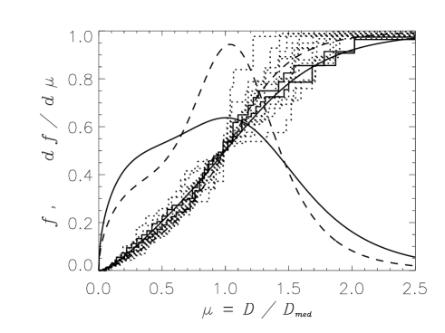
Figure 8: Cumulative and differential distributions, $f$ and $df/d\mu$, of the LCRS areas covered by voids as function of the normalized void size $\mu=D/D_{med}$. The solid histograms show the better sampled data sets 7 and 8, whereas the dotted ones stem from the diluted galaxy samples that scatter especially for large values of $\mu$. The monotonicly increasing solid curve provides a fit of the mean behavior, the monotonic dashed lines shows the behavior of Poisson samples. The peaked solid and dashed lines are differential size distributions from the data and from a set of Poisson samples, respectively.

A similarly important result of the present study is the derivation of a simple scaling relation (2) of the void sizes that give a cumulative voids coverage of 25%, 50%, and 75% in the galaxy distribution as shown in Fig. 4. The residual void size $D_{0}\approx 12\pm 3$ $h^{-1}$Mpc for the mean and the increase rate $\nu\approx 1$ in diluted samples characterize the hierarchy of voids in the LCRS. The void size distribution depends much more on the mean galaxy density than on the size of the survey volume or on the absolute magnitude of the galaxy sample. In fact, we only discussed the density dependence since only this dependence can be derived from the given data sets with high statistical significance. The strong suppression of the voids with sizes $D>2.5D_{med}$ underlines the fact that the size of the LCRS is large enough to get a reasonable estimate of the abundance of large voids and indicates a transition of the galaxy distribution to a homogeneous distribution at larger scales.

A further important point concerns the independence of the void size distribution with regard to the absolute magnitude range of the selected galaxies – e.g., the comparison of the void sizes in the data sets 1, 9, 11, 12, and 13. There, the median void sizes are similar, and only the maximum void sizes differ by about 15%. We ascribed it to the different depth of the data sets, but we should keep in mind that a larger volume corresponds in general to brighter galaxies. Disentangling both effects requires the extension of redshift surveys to a larger magnitude range, where even a small extension promises some progress as the comparison of the fields sampled partly with the 50 fiber spectrograph and the data from the $-12^{\circ}$ slice which is sampled completely with the 112 fiber spectrograph (sets 7, 8, 9, and 14) demonstrates.

The self-similarity of the void distribution in the LCRS is illustrated in Figs. 3 and 7, which show quite comparable shapes. The key dependence on the mean galaxy density is illustrated in Fig. 4 and in the two-parameter fit of the median and quartile void size distributions by the relations Eq. (2). Such relations are well reproduced by the hierarchical clustering in CDM models as the parameters in Table 2 demonstrate. The void distribution provides a sensitive test of these models. The dependence of the void statistics on the threshold criterion for the mock galaxy indentification shows that the galaxy biasing has a stronger influence than do cosmological parameters like the mean matter density or the precise form of the primordial power spectrum.

References

- Baugh (1996) Baugh C. M., 1996, MNRAS, 280, 267
- Bouchet et al. (1993) Bouchet F., Strauss M. A., Davis M., Fisher K. B., Yahil A., Huchra J. P., 1993, ApJ, 417, 36
- Bunn & White (1997) Bunn E. F., White M., 1997, ApJ, 480, 6
- Cen & Ostriker (1999) Cen R., Ostriker J. P., 1999, ApJ, 514, 1
- Chincarini & Rood (1979) Chincarini G., Rood H. J., 1979, ApJ, 230, 648
- Cole et al. (1998) Cole S., Hatton S., Weinberg D. H., Frenk C. S., 1998, MNRAS, 300, 945
- Coles, Melott & Shandarin (1993) Coles P., Melott A. L., Shandarin S. F., 1993, MNRAS, 260, 765
- da Costa et al. (1994) da Costa L. N., Geller M. J., Pellegrini P. S., Lathan D. W., Fairall A. P., Marzke R. O., Willmer C. N. A., Huchra J. P., Calderon J. H., Ramella M., Kurtz M. J., 1994, ApJ, 424, L1
- de Lapparent, Geller & Huchra (1986) de Lapparent V., Geller M. J., Huchra J. P., 1986, ApJ, 302, L1
- Doroshkevich et al. (1999) Doroshkevich A. G., Müller V., Retzlaff J., Tuchaninov V., 1999, MNRAS 306, 575
- Einasto, Jõeveer & Saar (1980) Einasto J., Jõeveer M., Saar E., 1980, MNRAS, 193, 353
- Einasto, Einasto & Gramann (1989) Einasto J., Einasto M., Gramann M., 1989, MNRAS, 238, 155
- Einasto et al. (1991) Einasto J., Einasto M., Gramann M., Saar E., 1991, MNRAS, 248, 593
- Einasto et al. (1999) Einasto J., Einasto M., Tago E., Müller V., Knebe A., Cen R., Starobinsky A. A., Atrio-Barandela F., 1999, ApJ, 515, 456
- Eke, Cole & Frenk (1996) Eke V., Cole S., Frenk C. S., 1996, MNRAS, 282, 263
- El-Ad & Piran (1997) El-Ad H., Piran T., 1997, ApJ, 491, 421
- El-Ad, Piran & da Costa (1997) El-Ad H., Piran T., da Costa L. N., 1997, MNRAS, 287, 790
- El-Ad & Piran (2000) El-Ad H., Piran T., 2000, MNRAS, 313, 553
- Ghigna et al. (1994) Ghigna S., Borgani S., Bonometto S., Guzzo L., Klypin A., Primack J., Giovanelli R., Haynes M., 1994, ApJ, 437, 71
- Ghigna et al. (1996) Ghigna, S., Bonometto, S., Retzlaff, J., Gottlöber, S., Murante, G., 1996, ApJ, 469, 40
- Gott, Melott & Dickinson (1986) Gott J R., Melott A. L., Dickinson M., 1986, ApJ, 306, 341
- Gregory & Thompson (1978) Gregory S. A., Thompson L. A., 1978, ApJ, 222, 784
- Jing et al. (1994) Jing J. P., Mo H. J., Börner G., Fang L. Z., 1994, A&A, 284, 703
- Jing, Mo & Börner (1999) Jing J. P., Mo H. J., Börner G., 1998, A&A, 494, 1
- Jõeveer et al. (1978) Jõeveer M., Einasto J., Tago E., 1978, MNRAS, 185, 357
- Kates et al. (1995) Kates R., Müller V., Gottlöber S., Mücket J. P., Retzlaff J., 1995, MNRAS, 277, 1254
- Kauffmann & Fairall (1991) Kauffmann G., Fairall A. P., 1991, MNRAS, 248, 313
- Kauffmann & Melott (1992) Kauffmann G., Melott A. L., 1992, ApJ, 393, 415
- Kirshner et al. (1981) Kirshner R. P., Oemler A., Schechter P. L., Shectman S. A., 1981, ApJ, 248, L57
- Lee & Shandarin (1998) Lee J., Shandarin S. F., 1998, ApJ, 507, L75
- Lin et al. (1996) Lin H., Kirshner R. P., Shectman S. A., Landy S. D., Oemler A., Tucker D. L., Schechter P. L., 1996, ApJ, 464, L60
- Lindner et al. (1995) Lindner U., Einasto J., Einasto M., Freudling W., Fricke K., Tago E., 1995, A&A, 301, 329
- Little & Weinberg (1994) Little B., Weinberg D. H., 1994, MNRAS, 267, 605
- Madsen et al. (1998) Madsen A., Doroshkevich A. G., Gottlöber S., Müller V., 1998, A&A, 329, 1
- Mann, Peacock & Heavens (1998) Mann R. G., Peacock J. A., Heavens A. F., 1998, MNRAS, 293, 209
- Mattig (1958) Mattig W., 1958, Astr.Nachr., 284, 109
- Melott et al. (1983) Melott, A., Einasto, J., Saar, E., Suisalu, I., Klypin, A.A., Shandarin, S.F., 1983, Phys.Rev.Lett., 51, 935
- Müller et al. (1998) Müller V., Doroshkevich A.G., Retzlaff J., & Turchaninov V.I., 1998, in Giuricin G., Mezzetti M., Salucci P., eds., Observational Cosmology: The Development of Galaxy Systems, ASP Conf. Ser. 176, San Francisco, 297
- Popescu, Hopp & Elsässer (1997) Popescu C. C., Hopp U., Elsässer H., 1997, A&A, 325, 881
- Press, et al. (1992) Press W. H., Teukolsky S. A., Vetterling W. T., Flannery B. P., 1992, Numerical Recipes, Cambridge Univ. Press
- Retzlaff et al. (1998) Retzlaff J., Borgani S., Gottlöber S., Klypin A., Müller V., 1998, NewA, 3, 631
- Ryden & Turner (1984) Ryden B. S., Turner E. L., 1984, ApJ, 287, L59
- Shectman et al. (1996) Shectman S. A., Landy S. D., Oemler A., Tucker D. L., Lin H., Kirshner R. P., Schechter P. L., 1996, ApJ, 470, 172
- Tarenghi et al. (1979) Tarenghi M., Tifft W. G., Chincarini G., Rood H. J.,Thomson L. A. 1979, ApJ, 234, 793
- Tully & Fisher (1978) Tully R. B., Fisher J. R., 1978, in Longair M. S., Einasto J., The Large Scale Structure of the Universe, Reidel, Dordrecht, 267
- Tucker et al. (1997) Tucker D. T., Oemler A., Kirshner R. P., Lin H., Shectman S. A., Landy S. D., Schechter P. L., Müller V., Gottlöber S., Einasto J., 1997, MNRAS 285, L5
- Vogeley, Geller & Huchra (1991) Vogeley M., Geller M. J., Huchra J. P., 1991, ApJ, 382, 44
- Vogeley et al. (1994) Vogeley M., Geller M. J., Park C., Huchra J. P., 1994, AJ, 108, 745
- Weinberg, Hernquist & Katz (1997) Weinberg D. H., Hernquist L., Katz N. J., 1994, ApJ, 477, 8
- White (1979) White S. D. M., 1979, MNRAS, 186, 145
- Zel’dovich (1970) Zel’dovich, Ya B., 1970, A&A, 5, 20
- Zel’dovich, Einasto & Shandarin (1982) Zel’dovich, Ya B., Einasto J., Shandarin I. D., 1982, Nature, 300, 407