EUV FLARE ACTIVITY IN LATE-TYPE STARS

Abstract

Extreme Ultraviolet Explorer Deep Survey observations of cool stars (spectral type F to M) have been used to investigate the distribution of coronal flare rates in energy and its relation to activity indicators and rotation parameters. Cumulative and differential flare rate distributions were constructed and fitted with different methods. Power laws are found to approximately describe the distributions. A trend toward flatter distributions for later-type stars is suggested in our sample. Assuming that the power laws continue below the detection limit, we have estimated that the superposition of flares with radiated energies of about $10^{29}-10^{31}$ ergs could explain the observed radiative power loss of these coronae, while the detected flares are contributing only $\approx 10$ %. While the power-law index is not correlated with rotation parameters (rotation period, projected rotational velocity, Rossby number) and only marginally with the X-ray luminosity, the flare occurrence rate is correlated with all of them. The occurrence rate of flares with energies larger than $10^{32}$ ergs is found to be proportional to the average total stellar X-ray luminosity. Thus, energetic flares occur more often in X-ray bright stars than in X-ray faint stars. The normalized occurrence rate of flares with energies larger than $10^{32}$ ergs increases with increasing $L_{\mathrm{X}}/L_{\mathrm{bol}}$ and stays constant for saturated stars. A similar saturation is found below a critical Rossby number. The findings are discussed in terms of simple statistical flare models in an attempt to explain the previously observed trend for higher average coronal temperatures in more active stars. It is concluded that flares can contribute a significant amount of energy to coronal heating in active stars.

1 INTRODUCTION

Stellar activity of “normal” stars has been explored extensively in the X-ray regime for more than two decades (e.g., Vaiana et al., 1981; Linsky, 1985). The chromospheres and coronae of some late-F to M main-sequence stars have been found to show enhanced magnetic activity. The latter is underlined by enhanced activity indicators such as the X-ray luminosity $L_{\mathrm{X}}$, its ratio to the bolometric luminosity $L_{\mathrm{X}}/L_{\mathrm{bol}}$, the presence of flares in the optical $U\!$ band (and in other wavelength regions), flux variations in chromospheric lines, spots on the stellar surface, etc. A dynamo mechanism is thought to be the primary cause for stellar and solar activity as suggested by the empirical relation between rotation and activity (for a recent review, see Simon, 2000). Rotation parameters (such as the rotation period, the Rossby number, or the angular velocity) are therefore prime parameters that determine the stellar activity level.

Stellar rotation was proposed to determine the level of activity of solar-type stars by Kraft (1967). Quantitative relationships between activity indicators and rotation parameters (e.g., Skumanich, 1972; Pallavicini et al., 1981; Walter, 1982; Noyes et al., 1984; Randich et al., 1996) provide information on the physical origin of stellar activity. In a study of X-ray emission from stars, Pallavicini et al. (1981) found that X-ray luminosities of late-type stars are dependent on the projected rotational velocity but are independent of bolometric luminosity. Walter & Bowyer (1981) and Walter (1981) presented observational evidence that RS CVn systems and G-type stars show a quiescent $L_{\mathrm{X}}/L_{\mathrm{bol}}$ ratio proportional to their angular velocity. However, in the same series of papers, Walter (1982) proposed that the simplistic view of a power-law dependence should be replaced by either a broken power law or by an exponential dependence of $L_{\mathrm{X}}/L_{\mathrm{bol}}$ on the angular velocity. This led to the concept of saturation of stellar activity (Vilhu, 1984; Vilhu & Walter, 1987) at high rotation rate. Noyes et al. (1984) suggested that the Rossby number $R_{0}$ (defined as the ratio $P/\tau_{\mathrm{c}}$ of the rotation period $P$ and the convective turnover time $\tau_{\mathrm{c}}$) mainly determines the surface magnetic activity in lower main-sequence stars. Stȩpień (1993) showed that, for main-sequence late-type stars, $R_{0}$ correlates with activity indicators better than $P$ does.

Flares are direct evidence of magnetic activity in stellar atmospheres. They are also in the center of the debate on the origin of coronal heating. Although several possible heating mechanisms have been identified (e.g., Ionson, 1985; Narain & Ulmschneider, 1990; Zirker, 1993; Haisch & Schmitt, 1996), there is increasing evidence that flares act as heating agents of the outer atmospheric layers of stars. A correlation between the apparently non-flaring (“quiescent”) coronal X-ray luminosity $L_{\mathrm{X}}$ and the stellar time-averaged $U$-band flare luminosity (Doyle & Butler, 1985; Skumanich, 1985) suggests that flares can release a sufficient amount of energy to produce the subsequently observed quiescent coronal emission. Robinson et al. (1995, 1999) found evidence for numerous transition region (TR) flares in CN Leo and YZ CMi. Further evidence for dynamic heating has been found in broadened TR emission line profiles (Linsky & Wood, 1994; Wood et al., 1996) that were interpreted in terms of a large number of explosive events.

Stellar X-ray and EUV flares have been found to be distributed in energy according to a power law (see Collura, Pasquini, & Schmitt, 1988; Audard, Güdel, & Guinan, 1999; Osten & Brown, 1999), similar to solar flares (e.g, Crosby, Aschwanden, & Dennis, 1993). One finds, for the flare rate $dN$ within the energy interval [$E,E+dE$],

$$\frac{dN}{dE}=k_{1}E^{-\alpha}.$$ (1)

The cumulative distribution for $\alpha>1$ is defined by

$$N(>E) = \int_{E}^{\infty}\frac{dN}{dE^{\prime}}dE^{\prime},$$ (2a)

$$= k_{2}E^{-\alpha+1},$$ (2b)

where the normalization factors $k_{1}$ and $k_{2}=k_{1}/\left(\alpha-1\right)$ are constants. For $\alpha>2$, an extrapolation to flare energies below the instrumental detection limit could be sufficient to produce a radiated power equivalent to the X-ray luminosity $L_{\mathrm{X}}$ of the quiescent corona,

$$L_{\mathrm{X}} = \int_{E_{\mathrm{min}}}^{E_{\mathrm{max}}}\frac{dN}{dE}E~{}dE,$$ (3a)

$$= k_{2}\frac{\alpha-1}{\alpha-2}\left(E_{\mathrm{min}}^{2-\alpha}-E_{\mathrm{max}}^{2-\alpha}\right),$$ (3b)

where $E_{\mathrm{max}}$ is the energy of the most energetic relevant flare. Small values of the minimum flare energy $E_{\mathrm{min}}$ then can lead to an arbitrarily large radiated power. Thus, as pointed out by Hudson (1991), it is crucial to investigate whether the solar (and stellar) flare rate distributions in energy steepen at lower energies. Parker (1988) suggested that the heating of the quiescent solar corona could be explained by “microflares”. In the solar context, several estimates of the power-law index have recently been given. For “normal” flares, $\alpha\approx 1.5-1.8$ (Crosby et al., 1993); it takes different values for smaller flare energies, from $\alpha\approx 1.6$ for small active-region transient brightenings (Shimizu, 1995) to $\alpha=2.3-2.6$ for small events in the quiet solar corona (Krucker & Benz, 1998), and other “intermediate” values (e.g., Porter, Fontenla, & Simnett, 1995; Aschwanden et al., 2000; Parnell & Jupp, 2000). Stellar studies on flare occurrence distributions in X-rays are rare, probably due to the paucity of stellar flare statistics. Using EXOSAT data, Collura et al. (1988) found a power-law index $\alpha$ of 1.52 for soft X-ray flares on M dwarfs. Osten & Brown (1999) reported $\alpha=1.6$ for flares in RS CVn systems observed with EUVE. On the other hand, Audard et al. (1999) found a power-law index $\alpha\approx 2.2\pm 0.2$ for two young active solar analogs.

In this paper, we present a follow-up study of Audard et al. (1999) for EUVE observations of active late-type main-sequence stars. Together with an investigation of coronal heating by flares, a more general picture of the relation between flares and stellar activity in general is developed. Section 2 presents the method for the data selection and reduction, section 3 explains the construction of cumulative and differential flare rate distributions in energy. Section 4 provides the methodology for fitting the distributions, while section 5 explores quantitatively the correlations between various physical parameters. Finally, section 6 gives a discussion of the results, together with conclusions.

2 DATA SELECTION AND REDUCTION

We use data from the Extreme Ultraviolet Explorer (EUVE, e.g. Malina & Bowyer, 1991) to study the contribution of flares to the observable EUV and X-ray emission from stellar coronae. In order to identify a sufficient number of flares in the EUVE Deep Survey (DS) light curves, data sets with more than 5 days of monitoring, or with a significant number of flares (more than ten flares identified by eye) were selected. Active coronal sources were our prime choice, as these stars often show several distinct stochastic events. We have focused our analysis on young, active stars that do not display rotationally modulated light curves and that can be considered as single X-ray sources. Some stars in the sample are detected or known binary systems, in which only one of the components is believed to contribute significantly to the EUV and X-ray emitted radiation. If a star was observed several times (more than a few days apart), we considered the different data sets as originating from different coronal sources, as the activity level of these stars is usually not identical at two different epochs. We carefully checked the DS data and rejected data that presented evident problems, such as “ghost” images in the DS remapped event files, or incursions into the DS “dead spot”. The final list contains 12 stellar sources (1 F-type, 4 G-type, 2 K-type, and 5 M-type coronal sources). We do not claim our sample to be complete in any sense. However, this sample is representative of the content of the magnetically active cool main-sequence stellar population in the EUVE archive. Table EUV FLARE ACTIVITY IN LATE-TYPE STARS gives the name of the stellar source (Col. 1), its spectral type (Col. 2), its distance $d$ in parsecs from Hipparcos (Perryman et al. 1997; except for AD Leo and CN Leo which are from Gliese & Jahreiss 1991; Col. 3), the rotation period $P$ in days together with its reference (Cols. 4 & 5), the projected rotational velocity and its reference (Cols. 6 & 7), the color index B V${}^{\ref{47casdef}}$ and the visual magnitude $V$ from Hipparcos (Perryman et al. 1997; except for AD Leo and CN Leo for which data were retrieved from Simbad; Cols. 8 & 9), the mean DS count rate (Col. 10), the derived (see below) EUV+X-ray (hereafter “coronal”) luminosity in the 0.01–10 keV energy range (Col. 11), and the EUVE observing window (Col. 12).

We have made extensive use of the data from the EUVE archive located at the Multimission Archive at the Space Telescope Science Institute (STScI). DS Remapped Archive QPOE files were rebuilt using the euv1.8 package within IRAF${}^{\ref{aura}}$. Light curves (Fig. EUV FLARE ACTIVITY IN LATE-TYPE STARS) were created using a DS background region ten times larger than the source region area. Event lists were extracted from the source region for further analysis. Thanks to the sufficiently large count rates of our sources, the contribution of the DS background was very low, and could be neglected (after a check for its constancy). Also, with our analysis method, flare-only count rates (count rates above the “quiescent” level) were required; therefore the small contribution of the background was eliminated in any case. Event and Good Time Interval (GTI) files were then read and processed with a flare identification code. Audard et al. (1999) explain in detail the procedure applied to identify flares in the DS event files. In brief, the method, adapted from Robinson et al. (1995), performs a statistical identification of flares. It assigns occurrence probabilities to light-curve bins. Note that several time bin lengths and time origins for the binning are used so that the identification of flares is not dependent on the choice of these parameters. Note also that, due to gaps between GTIs, the effective exposure of a bin had to be taken into account. We refer to Robinson et al. (1995) and Audard et al. (1999) for more details.

Figure EUV FLARE ACTIVITY IN LATE-TYPE STARS (upper panels) shows background-subtracted EUVE DS light curves for some data sets. Only for plotting purposes, the data have been binned to one bin per orbit ($P_{\mathrm{orb}}=96$ min). Note that for our data analysis, we have not restricted ourselves to the above bin size: bin durations from 1/5 to twice the orbital period have been used (see Fig. EUV FLARE ACTIVITY IN LATE-TYPE STARS). The lower panels show the corresponding “significance plots”, which give the probability for the presence of quiescent bins as a function of time (x-axis) and bin size (y-axis). The flare significance increases from light gray to black. Physical parameters (start time, end time and total duration) were determined from smoothed high-resolution light curves, using a Gaussian fit to the flares above a smooth lower envelope characterizing the quiescent contribution. Thus the start and end times of a flare were defined as the times separated from the maximum by 2 $\sigma$, where $\sigma$ is the standard deviation of the Gaussian function. Within this interval, we calculated a mean flare count rate above the quiescent emission by subtracting the mean background levels just before and after the flare, and multiplied it by the flare total duration to derive the total number of flare counts $C$. We then used a constant count-to-energy conversion factor ($f=1.06\times 10^{27}\;\mathrm{ergs\;ct^{-1}\;pc^{-2}}$) together with the source distance $d$ to derive the total energy $E$ radiated in the EUV and X-rays,

$$E=C\times f\times\left(4\pi d^{2}\right).$$ (4)

We derived the conversion factor $f$ from mean DS count rates of archival EUVE cool-star data sets and published X-ray luminosities (Pallavicini et al. 1988; van den Oord, Mewe, & Brinkman 1988; Pallavicini, Tagliaferri, & Stella 1990; Dempsey et al. 1993a, b; Schmitt, Fleming, & Giampapa 1995; Monsignori Fossi et al. 1996; Dempsey et al. 1997; Tagliaferri et al. 1997; Audard et al. 1999; Hünsch et al. 1999; Sciortino et al. 1999). We corrected the published X-ray luminosities to the new, Hipparcos-derived distances (Perryman et al., 1997). Then, using a typical model for young active stars (2-temperature collisional ionization equilibrium MEKAL model [$T_{1}=0.6$ keV, $T_{2}=2.0$ keV] with the iron abundance $\mathrm{Fe}=0.3$ times the solar photospheric value), we estimated factors to apply to the published luminosities in order to convert them to 0.01–10 keV luminosities. We finally defined the conversion factor $f$ as the mean ratio between the observed fluxes $L_{\mathrm{X}}/(4\pi d^{2})$ and the mean DS count rates $\mu$. Note that for our targets, the corona radiates mostly in the X-ray band ($\approx 0.1-5$ keV) rather than in the EUV band.

3 FLARE OCCURRENCE RATE DISTRIBUTIONS

Cumulative flare rate distributions in energy were constructed for each source (Fig. EUV FLARE ACTIVITY IN LATE-TYPE STARS). Similarly to Audard et al. (1999), we applied a correction to the effective rate of identified flares. For each cumulative distribution, the flare rate at the energy of the second-largest flare was corrected by a factor $D_{\mathrm{total}}/(D_{\mathrm{total}}-D_{\mathrm{largest}})$, where $D_{\mathrm{total}}$ is the total observing time span, and $D_{\mathrm{largest}}$ is the total duration of the largest flare. Analogously, the correction for the third-largest flare took into account the total durations of the largest and second-largest flares, and so on. This correction was necessary since usually more than 50 % of the DS light curves were occupied by identified flares, i.e. it is common for flares to overlap in time.

For each cumulative distribution, we have two series of parameters, namely the flare energy ($E_{i}$) and the flare rate at this energy ($s_{i}$), with the indices running from 0 (largest-energy flare, $s_{0}=1/D_{\mathrm{total}}$ by definition) to $M$ (lowest-energy flare). The cumulative occurrence rates $N(>E_{i})$, i.e., the rate of flares per day with energies exceeding $E_{i}$, were defined as

$$N(>E_{0}) = \frac{1}{D_{\mathrm{total}}}=s_{0},$$ (5a)

$$N(>E_{i}) = N(>E_{i-1})+s_{i},\quad i=1,\ldots,M.$$ (5b)

We then constructed differential distributions. For the energy interval [$E_{i},E_{i+1}$], we defined differential flare occurrence rates ($n_{i}$) as

$$n_{i}=\frac{s_{i}}{E_{i}-E_{i+1}},\quad i=0,\ldots,M-1.$$ (6)

We calculated uncertainties for the flare occurrence rates per unit energy; we assumed that each number of flares ($s^{\prime}_{i}=s_{i}\times D_{\mathrm{total}}$) with energy $E_{i}$ has an uncertainty $\Delta s^{\prime}_{i}$ estimated from a Poisson distribution. This approximation accounts for the larger relative uncertainty ($\Delta s^{\prime}_{i}/s^{\prime}_{i}$) of the number of detected flares at higher flare energies than at lower flare energies. However, instead of setting $\Delta s^{\prime}_{i}=\sqrt{s^{\prime}_{i}}$, we have used the approximations proposed by Gehrels (1986), who showed that for small $k$ following a Poisson distribution, the 1 $\sigma$ upper error bar can be approximated with $1+\left(k+3/4\right)^{1/2}$, while the the 1 $\sigma$ lower error bar is still approximated by the usual definition $\sqrt{k}$. Therefore, we have defined $\Delta s^{\prime}_{i}$ as the geometrical mean of the upper and lower error bars:

$$\Delta s^{\prime}_{i}=\left\{\sqrt{s^{\prime}_{i}}\times\left(1+\sqrt{s^{\prime}_{i}+\text@frac{3}{4}}\right)\right\}^{1/2}.$$ (7)

It follows that each differential occurrence rate $n_{i}$ has an uncertainty $\Delta n_{i}$ equal to

$$\Delta n_{i}=\frac{\Delta s^{\prime}_{i}/D_{\mathrm{total}}}{E_{i}-E_{i+1}}.$$ (8)

4 FITS TO THE DISTRIBUTIONS

4.1 Cumulative Distributions

The power-law fitting procedure to the cumulative flare occurrence rate distributions is adapted from Crawford, Jauncey, & Murdoch (1970). This method is based on a maximum-likelihood (ML) derivation of the best-fit power-law index $\alpha$. The best-fit normalization factors $k_{2}$ (see eq. [2b]) were then computed; using equation (3b), the minimum flare energy $E_{\mathrm{min}}$ required for the power law to explain the mean observed radiative energy loss ($L_{\mathrm{X}}$) was calculated, assuming that the cumulative flare occurrence rate distribution in radiated energy follow the same power law below the flare energy detection limit:

$$E_{\mathrm{min}}=\left\{\frac{L_{\mathrm{X}}}{k_{2}}\left(\frac{\alpha-2}{\alpha-1}\right)+E_{\mathrm{max}}^{2-\alpha}\right\}^{1/(2-\alpha)},$$ (9)

where the coronal luminosity $L_{\mathrm{X}}$ was estimated from $\mu$, the mean DS count rate,

$$L_{\mathrm{X}}=\mu\times f\times\left(4\pi d^{2}\right).$$ (10)

Columns 2 and 3 of Table 2 give the power-law indices $\alpha$ of the cumulative distributions, and the corresponding minimum flare energies $E_{\mathrm{min}}$. The best-fit power-law indices $\alpha$ derived from simple linear fits ($\chi^{2}$ method) in the $\log N(>E)-\log E$ plane have been added for comparison in Column 4.

We find a possible trend for decreasing power-law indices with increasing color indices; sources of spectral type F or G tend to show indices above the critical value of 2, although $\alpha<2$ is acceptable within the 1 $\sigma$ confidence range (except for the F star HD 2726). On the other hand, K and M stars show various power-law indices, with $\alpha>2$ being usually marginally acceptable, although some individual sources show best-fit values above 2. The minimum flare energies $E_{\mathrm{min}}$ can be associated with relatively small stellar flare energies. In the solar context, however, they correspond to medium-to-large flares ($E\approx 10^{29}-10^{31}$ ergs).

4.2 Differential Distributions

Our cumulative distributions do not account for uncertainties in the flare occurrence rates. Differential distributions allow us to avoid this effect, and they include uncertainties in a natural way (see section 3). Therefore, we propose to use this different approach in order to compare the results. The differential distributions were transformed into FITS files and were read into the XSPEC 10.00 software (Arnaud, 1996). Due to the characteristics of XSPEC, energy bins were created in which each bin $\delta E_{i}$ is defined as the interval between two consecutive flare energies (namely $\delta E_{i}=[E_{i+1},E_{i}]$, $i=0,\ldots,M-1$). Finally, a power-law fit (implemented in the software, using the $\chi^{2}$ minimization method) was performed for each distribution. To estimate the uncertainties derived for the index $\alpha$, confidence ranges for a single parameter were calculated by varying the index $\alpha$ and fitting the distribution until the deviation of $\chi^{2}$ from its best-fit value reached $\delta\chi^{2}=1.00$. The power-law indices and their corresponding confidence ranges can be found in Col. 5 (Table 2). Note that the small “signal-to-noise” of the distributions did not allow us to better determine the confidence ranges. Relative uncertainties of the $n_{i}$ values were usually larger than 50 %, reaching about 150 % at most. We also note that the values of $\alpha$ derived from fits to the cumulative distributions are similar to those derived from fits to differential distributions; confidence ranges for the second method are, however, larger and originate from the inclusion of uncertainties in the flare rates, together with the small number of detected flares. A strong support for this statement comes from the confidence range derived for $\kappa$ Cet 1994. Only four energy bins were used, leading to large confidence ranges and an unconstrained upper limit for $\alpha$.

4.2.1 Combined Data Sets

A possible dependence of $\alpha$ with the stellar spectral type has been mentioned above. To test this trend further and also to obtain tighter results for our power-law fits, we have performed simultaneous fits to the differential distributions within XSPEC. In brief, all data sets belonging to a spectral type (we combined the only F star with the G-type sources) were fitted simultaneously with power laws of identical index $\alpha$ and one normalization factor for each data set. Note that, with this procedure, the confidence range for $\alpha$ is better determined than in the case of individual distribution fits. The implicit hypothesis of this procedure assumes that the coronae of stellar sources within a given spectral class behave similarly, without any influence by age, rotation period, projected stellar velocity, etc. Columns 6 & 7 of Table 2 show the result of the simultaneous fits, together with 68.3 % confidence ranges for a single parameter. Again, we find a trend for lower indices at later spectral types, although the significance is marginal at best.

5 CORRELATIONS WITH PHYSICAL PARAMETERS

We have explored correlations of the best-fit power-law indices $\alpha$ and occurrence rates of flares showing energies larger than a typical energy observed in our data ($E_{\mathrm{c}}=10^{32}$ ergs) with rotation parameters (rotation period $P$, projected rotational velocity $v\sin i$, Rossby number $R_{0}$) and activity indicators (coronal luminosity $L_{\mathrm{X}}$, and its ratio $L_{\mathrm{X}}/L_{\mathrm{bol}}$ to the bolometric luminosity). Two nonparametric rank-correlation tests (Spearman’s $r_{\mathrm{S}}$ and Kendall’s $\tau$; Press et al. 1992) were used. These robust tests allow us to calculate correlation coefficients and to obtain a two-sided (correlation or anticorrelation) significance for the absence of correlation. Thus, a low correlation coefficient ($r_{\mathrm{S}}$ or $\tau$) can be associated with a high probability that the sample is not correlated. Note that Kendall’s $\tau$ is more nonparametric than Spearman’s $r_{\mathrm{S}}$ because it uses only the relative ordering of ranks instead of the numerical difference between ranks (Press et al., 1992). No uncertainty was included in the tests. In Table 3, we give the rank-correlation coefficients together with their two-sided significances in parentheses. We have defined two data groups for the tests. The first group (hereafter DG1) corresponds to power-law indices or flare rates derived from ML fits to the cumulative distributions, while data group 2 (hereafter DG2) corresponds to indices or flare rates derived from fits to the differential distributions.

5.1 Correlations of the Power-Law Index $\alpha$

5.1.1 Coronal Luminosity $L_{\mathrm{X}}$

Coronal luminosities (see eq. [10]) were used to test their correlation with $\alpha$ (Fig. EUV FLARE ACTIVITY IN LATE-TYPE STARS). For each data group, the significance levels (Table 3) are usually smaller than 5 %, the highest level reaching 10 %. Therefore, placing a limit of 5 % to the two-sided significance level, the correlation between $\alpha$ and $L_{\mathrm{X}}$ is marginally significant at best. Such a correlation can be explained as follows. For saturated stars ($L_{\mathrm{X}}\approx 10^{-3}L_{\mathrm{bol}}$), the X-ray luminosity should decline for stars with spectral type from F to M (hence increasing color index B V) because of the decrease of their bolometric luminosity. In section 4.2.1, we have found a suggestion that the power-law index $\alpha$ is weakly correlated with the stellar spectral type. Therefore, a weak correlation of $L_{\mathrm{X}}$ with $\alpha$ can be expected. Note that due to the scatter in the $L_{\mathrm{X}}/L_{\mathrm{bol}}$ ratio in our sample, this can lead to a scatter in the dependence of $L_{\mathrm{X}}$ on the spectral type, hence in the dependence of $L_{\mathrm{X}}$ on the index $\alpha$.

5.1.2 Ratio $L_{\mathrm{X}}/L_{\mathrm{bol}}$

We have tested the correlation between $L_{\mathrm{X}}/L_{\mathrm{bol}}$ and the power-law index. The bolometric luminosities were calculated from parameters in Table EUV FLARE ACTIVITY IN LATE-TYPE STARS and corresponding bolometric corrections. Two-sided significance levels (Table 3) show that the correlation between $L_{\mathrm{X}}/L_{\mathrm{bol}}$ and $\alpha$ is not significant.

5.1.3 Rotation Period $P$

For stars with known rotation periods (Table EUV FLARE ACTIVITY IN LATE-TYPE STARS), we have tested the correlation between the power-law index $\alpha$ and $P$. Note that for $\kappa$ Cet, for which there are two data sets, we have used weighted means of the indices $\alpha$. Our final sample then comprised 7 data points. From the two-sided significance levels, we can state that no correlation between the power-law index $\alpha$ and the rotation period $P$ is present in our sample (Table 3).

5.1.4 Projected Rotational Velocity $v\sin i$

Projected rotational velocities from Table EUV FLARE ACTIVITY IN LATE-TYPE STARS were used. We used the same procedure as above to calculate the weighted mean of $\alpha$ for $\kappa$ Cet; for the tests, the upper limits (GJ 411, CN Leo) have been omitted. Our sample then contained 8 data points for each data group. The two-sided significances for the present correlation tests (Table 3) imply the absence of a significant correlation between the power-law index $\alpha$ and the projected rotational velocity $v\sin i$ in our data sample.

5.1.5 Rossby Number $R_{0}$

We have used the available periods in Table EUV FLARE ACTIVITY IN LATE-TYPE STARS and have calculated the convective turnover times $\tau_{\mathrm{c}}^{\left(2\right)}$ (the number 2 refers to the ratio of the mixing length to the scale height) from the B V color index and equation (4) of Noyes et al. (1984) in order to derive $R_{0}$. The nonparametric tests again suggest an insignificant correlation between the index $\alpha$ and the Rossby number.

5.2 Correlations of the Flare Occurrence Rate

5.2.1 Flare Rate vs. $L_{\mathrm{X}}$

Figure EUV FLARE ACTIVITY IN LATE-TYPE STARS shows the occurrence rate of flares with energies larger than $10^{32}$ ergs ($E_{\mathrm{c}}$) versus the coronal luminosity $L_{\mathrm{X}}$. Quiescent X-ray luminosities (corrected to an energy range between 0.01 and 10 keV) taken from the literature (Collier Cameron et al., 1988; Pallavicini et al., 1990; Hünsch, Schmitt, & Voges, 1998; Hünsch et al., 1999) were also used for comparison (crosses), although they were not taken into account in the following tests. The evident correlation between $N(>E_{\mathrm{c}})$ and $L_{\mathrm{X}}$ is confirmed by Spearman’s $r_{\mathrm{S}}$ and Kendall’s $\tau$ tests. The former has rank-correlation coefficients of $0.95$ and $0.94$, with two-sided significances for deviation from zero of $2\times 10^{-6}$ and $4\times 10^{-6}$ for DG1 and DG2, respectively. The latter test has coefficients of $0.85$ and $0.82$, while significances are $1\times 10^{-4}$ and $2\times 10^{-4}$. This implies that a correlation between $L_{\mathrm{X}}$ and the flare occurrence rate is highly significant for our data sample (Figure EUV FLARE ACTIVITY IN LATE-TYPE STARS). The linear best-fit in the $\log-\log$ plane for DG1 is $\log N(>E_{\mathrm{c}})=(-26.7\pm 2.9)+(0.95\pm 0.10)\log L_{\mathrm{X}}$ (number of flares per day), while the best-fit for DG2 was $\log N(>E_{\mathrm{c}})=(-25.5\pm 2.8)+(0.90\pm 0.10)\log L_{\mathrm{X}}$, hence the relation between the flare rate and the luminosity is compatible with proportionality. Note that, as the correlation between $\alpha$ and $L_{\mathrm{X}}$ was marginal at best (section 5.1.1), we can safely state that proportionality exists between $L_{\mathrm{X}}$ and the normalization factor $k_{2}$ (and hence $k_{1}$).

5.2.2 Normalized Flare Rate vs. $L_{\mathrm{X}}/L_{\mathrm{bol}}$

The canonical saturation limit for stars with different spectral types has been found to appear at different $v\sin i$ (e.g., Caillault & Helfand, 1985; Stauffer et al., 1994; Randich et al., 1996; Stauffer et al., 1997), and therefore, based on the relation of Pallavicini et al. (1981) between $v\sin i$ and $L_{\mathrm{X}}$ for unsaturated stars, at different X-ray luminosities. Figure EUV FLARE ACTIVITY IN LATE-TYPE STARS shows the coronal luminosity $L_{\mathrm{X}}$ against the bolometric luminosity $L_{\mathrm{bol}}$. It emphasizes the different loci of our coronal sources with respect to saturation. Note that $L_{\mathrm{X}}/L_{\mathrm{bol}}$ ratios range from $\approx$$10^{-5}$ to $\approx$$10^{-3}$. For our correlation tests, we have normalized, for each source, the occurrence rates of flares with energies larger than $10^{32}$ ergs with the occurrence rate $N(>E_{\mathrm{c}})_{\mathrm{sat}}$ at the saturation turn-on for the given spectral type ($L_{\mathrm{X,sat}}=10^{-3}L_{\mathrm{bol}}$) derived from the best-fits to $N(>E_{\mathrm{c}})$ vs. $L_{\mathrm{X}}$ in the previous section. Thus, we are able to check whether or not the normalized flare occurrence rate stays constant at unity at activity saturation. Figure EUV FLARE ACTIVITY IN LATE-TYPE STARS suggests that it does and that the flare rate saturates at activity saturation. In the following sections, we will suggest that this effect is not biased by the absence of stars “beyond” saturation. Note a few discrepant features, such as for 47 Cas (point 2). Its point in DG2 is about 1/2 dex higher than in DG1. Since its index is larger ($\alpha\approx 2.6$) for DG2 than for DG1 ($\alpha\approx 2.2$), and since its minimum observed flare energy is about $10^{33}$ ergs, it follows that $N(>E_{\mathrm{c}})$ is larger for DG2 than for DG1. Similarly, CN Leo (points 11 & 12) has two different $\alpha$ indices for the 1994 and 1995 observations ($\alpha\approx 2.2\textrm{ and }1.5$). This large discrepancy (due to the flat low-energy end of the 1995 distributions) induces different normalized flare occurrence rates.

5.2.3 Normalized Flare Rate vs. Normalized $v\sin i$

As before, it was necessary to normalize the flare occurrence rates. In section 5.2.2, we have shown that, for our sample, the normalized flare occurrence rate does not show a trend to increase at saturation. However, our sample contains stars “beyond” saturation, i.e., stars that appear saturated ($L_{\mathrm{X}}/L_{\mathrm{bol}}\approx 10^{-3}$) but that rotate faster than a star at the onset of saturation. Therefore, we have normalized $v\sin i$ with $(v\sin i)_{\mathrm{sat}}$, where the latter were obtained from the Pallavicini et al. (1981) relation ($L_{\mathrm{X}}=1.4\times 10^{27}[v\sin i]^{1.9}$) at the saturation turn-on for each stellar spectral type. Stars at the saturation level thus have normalized velocities around 1, while those beyond that level have values significantly higher than 1 (Fig. EUV FLARE ACTIVITY IN LATE-TYPE STARS). In our sample, two stars show high values. The first is the bright K1 dwarf AB Dor, and the second is the M6 dwarf CN Leo, although its projected rotational velocity is an upper limit. Hence, AB Dor is the only star that supports the suggestion of constant normalized flare rates at $v\sin i$ saturation. However, in the following section, we will show that the result is also supported by a correlation with the Rossby number $R_{0}$, which is less dependent on spectral type. We have performed a fit to the data, assuming a saturation function of the type

$$\frac{N(>E_{\mathrm{c}})}{N(>E_{\mathrm{c}})_{\mathrm{sat}}}=1-\exp\left(-\frac{1}{\zeta}\frac{v\sin i}{(v\sin i)_{\mathrm{sat}}}\right),$$ (11)

with $\zeta$ as the single fit parameter. We derived $\zeta=0.56$ for DG1, and $\zeta=0.33$ for DG2. For the fits, we have used the estimated equatorial velocity for 47 Cas, the logarithmically averaged flare rate for $\kappa$ Cet, and we have not taken into account the upper limits for CN Leo and GJ 411.

5.2.4 Normalized Flare Rate vs. $R_{0}$

We have further tested the saturation of the flare rate using $R_{0}$. Compared to the normalized projected rotational velocity, the Rossby number does not contain the uncertainty due to the projection angle $i$. Furthermore, it does not need to be normalized as it already corresponds to a normalized rotation period. However, the rotation period is not available for each star of our sample. Figure EUV FLARE ACTIVITY IN LATE-TYPE STARS (upper and middle panels) suggests a saturation effect, although again only AB Dor supports it. Also, the $N(>E_{\mathrm{c}})/N(>E_{\mathrm{c}})_{\mathrm{sat}}$ vs. $R_{0}$ plots (upper and middle panels) are very similar to the well-known activity saturation relation with the Rossby number (lower panel of Figure EUV FLARE ACTIVITY IN LATE-TYPE STARS). Similarly to the normalized flare rate saturation, the luminosity saturation appears at $\log R_{0}<1.2$. Both the normalized flare rate and the luminosity decrease above this limit, as previously found for $L_{\mathrm{X}}/L_{\mathrm{bol}}$ (e.g, Randich et al., 1996; Stauffer et al., 1997). Two lines were overlaid for $\log R_{0}\geq 1.2$. The solid line corresponds to the best fit to the data of Randich et al. (1996, $\log L_{\mathrm{X}}/L_{\mathrm{bol}}=-4.4-1.12\log R_{0}$), while the dashed line corresponds to our best-fit solution, $\log L_{\mathrm{X}}/L_{\mathrm{bol}}=(-4.76\pm 0.30)-(1.72\pm 0.42)\log R_{0}$, with the ratios $L_{\mathrm{X}}/L_{\mathrm{bol}}$ of $\kappa$ Cet being logarithmically averaged. Our sample follows approximately the relation of Randich et al. (1996). Hence, together with the upper and middle panels, the lower panel of Figure EUV FLARE ACTIVITY IN LATE-TYPE STARS reinforces the suggestion that there is a saturation of the flare rate at the activity saturation.

5.3 Flare Power vs. $L_{\mathrm{X}}$

In Figure EUV FLARE ACTIVITY IN LATE-TYPE STARS, we have plotted the X-radiated power $P_{F}$ from the detected flares as a function of the average luminosity $L_{\mathrm{X}}$. There is an obvious correlation (Spearman: $r_{\mathrm{S}}=0.93$, $P[r_{\mathrm{S}}=0]=1.2\times 10^{-5}$; Kendall: $\tau=0.82$, $P[\tau=0]=2.1\times 10^{-4}$) between the parameters. This again demonstrates the importance of the flare contributions to the observed radiation from active coronae. Note that, for our sample and for our flare detection threshold, about 10 % of the X-ray luminosity originates from detected flares.

6 DISCUSSION AND CONCLUSIONS

In the present work we have investigated statistical properties of EUV flare events on time scales of days and weeks. Although the sensitivity of the EUVE DS instrument is quite limited, it provides long time series that are sufficient to draw rough conclusions on the statistical flare behavior of active stellar coronae.

The first aspect of interest is the distribution of flare energies. In the solar case, X-ray flares are distributed in energy according to a power law with a power-law index around 2 (e.g., Crosby et al., 1993). Many of the active stars studied here are quite different from the present-day Sun, with distinct coronal behavior. For example, high-energy particles are continuously present in their coronae as inferred from their steady gyrosynchrotron emission (e.g., Linsky & Gary, 1983; Güdel, 1994); quiescent coronal temperatures reach values of 20 MK which are typical on the Sun only in rather strong flares. Individual flare energies accessible and observed by EUVE in this study are, in several cases, not observed on the Sun at all. Since a limited amount of magnetic energy is available in the reconnection zones of the coronal magnetic fields, one would even expect some upper threshold to observable flare energies from solar-like stars (and therefore to the observed flare X-ray radiation).

Our investigation on active main-sequence stars has shown that, for the energy range observed, the flare occurrence rate distributions in energy can be fitted by power laws. We have not found significant evidence for broken power laws that indicate a threshold energy. The largest amount of radiated energy was found to be $10^{35}$ ergs in our flare sample, exceeding the X-ray output of very large solar flares by two to three orders of magnitude.

Measuring the value of the power-law indices of the distributions is pivotal for assessing the role of flares in coronal heating. The quite limited statistics make conclusions somewhat tentative, although we emphasize the following. The power-law indices definitely cluster around a value of 2; they may be slightly different for different stellar spectral types (Table 2). The stellar distributions are thus broadly equivalent to solar distributions, which implies that a) the cause of flare initiation in magnetically very active stars may be similar to the Sun, and b) that the trend continues up to energies at least two orders of magnitude higher than observed on the Sun. We are conversely motivated to extrapolate our distributions to lower energies given the rather large range over which solar flares follow a power law. Caution is in order, however, toward low-energy flares for which the distributions may steepen (Krucker & Benz, 1998).

Hudson (1991) argued that, for a power-law index above 2, an extrapolation to small flare energies could explain the radiated power of the solar corona. We derived (eq. [9]) the minimum flare energies $E_{\mathrm{min}}$ required for the power laws to explain our stellar X-ray luminosities (Table 2). For stars with $\alpha>2$ or just barely below $2$, minimum flare energies around $10^{29}-10^{31}$ ergs were obtained. Such energies correspond to intermediate solar flares. Explicit measurements of flare energies below our detection thresholds will however be required to conclusively estimate their contribution to the overall radiation.

We have found a trend for a flattening of the flare rate distributions in energy toward later spectral types. F and G-type stars tend toward power-law indices $>2$, while K and M dwarfs tend toward indices $<2$. If supported by further, more sensitive surveys, it suggests that flares play a more dominant role in the heating of F and G-type coronae, while they cannot provide sufficient energy to explain the observed radiation losses in K and M dwarfs. On the other hand, part of this trend could be due to the bias introduced by the identification method and the length of the GTIs. Although not found in our data, later-type (K and M-type) stars may show flares that are typically shorter than those of G dwarfs, partly because of the smaller distances of the stars that give access to less energetic (and therefore, as on the Sun, typically shorter) flares. But then the flare duration is smaller than the typical GTI gaps (about 3000 s) so that flares that occur between the GTIs remain completely undetected. This effect can considerably flatten the flare rate distributions.

Given that our study is restricted to flares with energies typically exceeding $10^{31}-10^{32}$ ergs, it is little suprising that the observed flare radiation amounts to only a fraction of the total EUV and X-ray losses. We infer an (observed) fraction of approximately 10 % relative to the average (quiescent) coronal luminosity. This lower limit will undoubtedly increase with better instrument sensitivity. Our study therefore clearly indicates that flares provide an important and significant contribution to the overall heating of active stellar coronae.

We have further explored whether statistical flare properties are correlated with some physical properties of the stars, such as activity indicators and rotation parameters. The power-law index $\alpha$ does not correlate with any of the rotation parameters ($P$, $v\sin i$, $R_{0}$) nor with the ratio $L_{\mathrm{X}}/L_{\mathrm{bol}}$. The absence of clear correlations suggest that the activity phenomena related to flares are similar on stars of all activity levels. A marginally significant correlation with the coronal luminosity was found. This result is probably related to the trend found for the dependence of $\alpha$ on the stellar spectral type.

On the other hand, the flare occurrence rate above a given lower energy threshold is correlated with each of the activity indicators and rotation parameters. A single power law ($N[>E_{\mathrm{c}}]\propto L_{\mathrm{X}}$) fits the correlation between flare rate and the coronal luminosity quite well, indicating that energetic flares occur more frequently in X-ray luminous stars than in X-ray weak stars. In order to compare the activity levels between stars of our sample, we have normalized the flare rate to its value that a star adopts at its saturation level. The normalized flare occurrence rate increases with increasing activity but stays constant for saturated stars. Flare rate saturation underlines the close relation between flares and the overall “quiescent” coronal emission. We now ask more specifically whether the apparently quiescent X-ray radiation could be related to the derived flare distributions.

In simple terms, we expect a larger magnetic filling factor on magnetically more active stars, or more numerous (or larger) active regions than on low-activity stars. A higher filling factor naturally implies a proportionally higher quiescent X-ray luminosity and proportionally more numerous flares, so that we expect a linear correlation between $L_{\mathrm{X}}$ and the flare rate. But what is the nature of the quiescent emission?

It is known from X-ray observations that the average quiescent coronal temperatures characteristically increase with increasing activity. The concept of an average coronal temperature is, however, somewhat problematic. Schrijver, Mewe, & Walter (1984) used single-$T$ fits to Einstein/IPC data that roughly imply that the total stellar volume emission measure in X-rays $\mathrm{EM_{\star}}$ is proportional to $T^{3}$ (as discussed in Jordan & Montesinos 1991). Since the radiative cooling function $\Lambda(T)$ in the range of interest ($3-30$ MK) scales approximately like $T^{-\phi}$ with $\phi\approx 0.3$ (Kaastra, Mewe, & Nieuwenhuijzen, 1996), we have for $L_{\mathrm{X}}$

$$L_{\rm X}\approx{\rm EM_{\star}}~{}\Lambda(T)\propto{\rm EM_{\star}}~{}T^{-\phi}$$ (12)

and hence $L_{\mathrm{X}}\propto T^{2.7}$. Considering that the typical coronal emission measure is distributed in temperature, multi-$T$ fits appear to better represent average coronal temperatures. Also, to disentangle functional dependencies from other stellar parameters (e.g., the stellar radius), a uniform sample of stars should be used. Güdel et al. (1997) derived two-temperature models from ROSAT data for a sample of stars that differ only in their activity levels but are otherwise analogs to the Sun. For the hotter component, they found $L_{\mathrm{X}}\propto T_{\rm hot}^{4.16-5.09}$, the range of the exponent illustrating two different spectral models applied. If, however, we compute the mean of the two temperatures weighted with the corresponding emission measures from their Table 3, we find $L_{\mathrm{X}}\propto T^{4.8}$ independent of the spectral model. The two more active stars for which ASCA 3-$T$ fits were available in Güdel et al. (1997) agree well with this trend (for cooler coronae, ASCA is not sufficiently sensitive to derive a coronal emission measure distribution). Note that the 3-$T$ fits in turn represent the derived emission measure distributions in Güdel et al. (1997) quite well. We therefore conclude that the emission-measure weighted average coronal temperature roughly scales as $L_{\rm X}\propto T^{4.8}$, although with a considerable uncertainty in the exponent.

Hearn (1975) and Jordan et al. (1987) discuss “minimum flux” coronae that follow a relation $\mathrm{EM_{\star}}\propto T^{3}g_{\star}$ where $g_{\star}$ is the stellar surface gravity. In a similar way, Rosner, Tucker, & Vaiana (1978) find scaling laws for closed static magnetic loops that relate external heating, loop pressure, loop-top temperature, and loop length. The two scaling laws combine to

$$\dot{E}_{\rm H}\propto{T^{21/6}\over L^{2}}$$ (13)

where $\dot{E}_{\rm H}$ is the heating rate, $T$ is the (dominating) loop-top temperature, and $L$ is the loop length. Schrijver et al. (1984), based on these scaling laws, conclude that different families of loops must be present on active stars. In either case, explaining the locus of the measured ($T$, $\mathrm{EM_{\star}}$) on the empirical relation requires an explanation for a specific amount of heating energy input to the system. Our investigation suggests that flare events contribute significantly to the observed overall emission. If the concept of a truly quiescent radiation is abandoned completely for magnetically active stars, then we may ask whether flares themselves can explain the observed relation between $\mathrm{EM_{\star}}$ and $T$ while at the same time accounting for the proportionality between flare rate and $L_{\mathrm{X}}$. We briefly discuss two extreme cases:

i) Filling factor-related activity. We first assume that flares are statistically independent and occur at many different, unrelated flare sites. The quiescent emission in this case is the superposition of all flare light curves. The proportionality between flare rate and $L_{\mathrm{X}}$ is simply due to more numerous flare loops on stars with higher magnetic filling factors (and hence higher activity), in which the explosive energy releases build up the observed loop emission measure. We ask whether the statistical flare distribution determines the average coronal temperature as well.

From our flare samples, we have found that the flare duration does not obviously depend on the flare energy (as typically found for impulsive flares on the Sun; Crosby et al. 1993). We therefore first assume one fixed time constant for all flares. For example, radiatively decaying flares with a similar evolution of coronal densities, abundances and temperatures show similar decay time scales. In this case, the single flare peak luminosity $\mathcal{L}_{\rm X}$ is proportional to the total radiated flare energy $E$. Further, for solar (and stellar) flares, a rough relation between peak emission measure $\mathrm{EM}$ and peak temperature $T$ has been reported by Feldman, Laming, & Doschek (1995). For the interesting range between $5-30$ MK, the relation can be approximated by

$$\mathrm{EM}=aT^{b}\quad{\rm[cm^{-3}]}$$ (14)

with $a\approx 10^{12}$ cm^-3, $b\approx 5\pm 1$, and $T$ measured in K. We approximate the flare contribution to the radiative losses by the values around flare peak. For the flare radiative losses, we have, equivalent to equation (12),

$$\mathcal{L}_{\rm X}\approx{\rm EM}~{}\Lambda(T)\propto{\rm EM}~{}T^{-\phi}$$ (15)

again with $\phi\approx 0.3$ over the temperature range of interest. With equations (14) and (15), we obtain

$$E\propto\mathcal{L}_{\rm X}\propto T^{b-\phi}.$$ (16)

To derive a characteristic, emission-measure weighted, time-averaged mean coronal temperature $\overline{T}$, we average over all flare temperatures $\left[T_{\mathrm{s}},T_{0}\right]$ by using their peak $\mathrm{EM}$ and their occurrence rates as weights:

$$\overline{T}=\frac{\int_{T_{\mathrm{s}}}^{T_{0}}T~{}{\rm EM(T)}~{}dN/dE~{}dE/dT~{}dT}{\int_{T_{\mathrm{s}}}^{T_{0}}{\rm EM(T)}~{}dN/dE~{}dE/dT~{}dT}.$$ (17)

Here, $T_{\mathrm{s}}$ represents the typical temperature of the smallest contributing flares. From equations (14)–(17), we obtain

$$\overline{T}=\frac{z}{z+1}~{}T_{0}~{}\frac{1-(T_{\mathrm{s}}/T_{0})^{z+1}}{1-(T_{\mathrm{s}}/T_{0})^{z}}$$ (18)

where

$$z=(2-\alpha)b-(1-\alpha)\phi.$$ (19)

Without loss of generality, we assume $T_{\mathrm{s}}=1$ MK. The upper temperature limit $T_{0}$ corresponds to the largest flare energy $E_{0}$ typically contributing to the apparently quiescent emission. Since the flare rate is given by the power law (eq. [1]), the characteristic value for $E_{0}$ scales like $k_{1}^{1/\alpha}$, i.e., with equation (16), $T_{0}\propto k_{1}^{1/(\alpha(b-\phi))}$. The normalization factor $k_{1}$ is proportional to the overall stellar X-ray luminosity $L_{\mathrm{X}}$ for given $\alpha$. The steepest dependence of $\overline{T}$ on $k_{1}$ is obtained in the limit of small $\alpha$, i.e. $z>0$, so that $\alpha<(2b-\phi)/(b-\phi)$, implying $\alpha\lesssim 2.1$. Then, for $T_{0}\gg T_{\mathrm{s}}$, we find $\overline{T}\propto T_{0}$, i.e., $L_{\rm X}\propto\overline{T}^{\beta}$ with $\beta=\alpha(b-\phi)$. For reasonable values of $\alpha=1.5-2.1$, we find $\beta\approx 5.5-12$, i.e., a dependence that is at least somewhat steeper than observed.

We can repeat the derivation under the assumption of some dependence between flare energy $E$ and duration $D$. Typically, larger flares last longer. The function $D(T)=D(E[T])$ should then be used as an additional weighting factor in equation (17). Assuming that $D\propto E^{1/2}$ (e.g., in the case of an energy-independent “flare curve shape”), we find $E\propto\mathcal{L}_{\mathrm{X}}^{2}$. In that case, equation (18) remains valid, while $z=(4-2\alpha)b-(3-2\alpha)\phi$ and $L_{\mathrm{X}}\propto\overline{T}^{\beta}$ with $\beta=2\alpha(b-\phi)$ for “small” $\alpha$, hence a steeper dependence on $\overline{T}$ than for the first case.

ii) Loop reheating. In the other extreme case, the flares repeatedly reheat the same coronal plasma in certain “active” loop systems (e.g., Kopp & Poletto, 1993). In that case, for most of the time the coronal loops fulfill a quasi-static approximation equivalent to the loop scaling law given by Rosner et al. (1978) (see Jakimiec et al., 1992). The situation is equivalent to steadily heated loops. The first scaling law of Rosner et al. (1978), $T_{\rm max}\propto(pL)^{1/3}$, implies EM $\propto T^{4}$ and hence $L_{\rm X}\propto T^{3.7}$ for a given loop length with $T$ in the range of interest. For loops exceeding the coronal pressure scale height, Schrijver et al. (1984) give an expression EM $\propto T^{5}$ (with other parameters fixed), and hence $L_{\rm X}\propto T^{4.7}$. In this limit, we attribute the higher temperatures of more active stars to higher reheating rates in a similar number of loops rather than to a larger number of statistically independent heating events in more numerous active regions or loops. The cause of an enhanced reheating rate on more active stars in a similar number of loop systems remains to be explained, however.

Comparing the observed average coronal temperatures with the two extreme results, we see that the observed trend lies in the middle between the extreme values. Flare heating is thus a viable candidate to explain the trends seen in $L_{\mathrm{X}}$ and in $T$, although it is not conclusive whether flares occur independently or whether they act as reheating agents of coronal loops. It appears unlikely that either extreme is appropriate. While a larger magnetic filling factor on more active stars undoubtedly produces more numerous active regions and thus a higher flare rate, the higher coronal filling factor is also likely to lead to more numerous reheating events. This is compatible with the observed trend between $L_{\rm X}$ and $\overline{T}$.

This study has shown that flares can provide a significant amount of energy to heat the coronae of active stars. Although the definite answer to which mechanism is responsible for coronal heating is not yet available, our data sample suggests that flares are promising contributors. Better sensitivity together with uninterrupted observations (such as those provided by the new generation of X-ray satellites XMM-Newton and Chandra) will be needed to solve part of the mystery. Our method is limited to flares explicitly detectable in the light curves. Alternative methods are available that model light curves based on statistical models. These investigations are the subject of a forthcoming paper (Drake et al., 2000).

Examples of light curves and significance plots.

The cumulative flare occurrence rate distributions for all twelve data sets.

Power-law index $\alpha$ vs. coronal $L_{\mathrm{X}}$.

Occurrence rate of flares with energies larger than $10^{32}$ ergs vs. coronal luminosity $L_{\mathrm{X}}$. Data group 1 corresponds to the rates derived from the fits to cumulative distributions, while data group 2 corresponds to the rates derived from the fits to differential distributions. The $\chi^{2}$ linear best-fits in the $\log-\log$ plane are shown as straight lines together with the analytical formulation. Crosses represent $L_{\mathrm{X}}$ values for these sources taken from the literature (see text).

Coronal luminosity $L_{\mathrm{X}}$ vs. bolometric luminosity $L_{\mathrm{bol}}$. The source identification numbers refer to Table EUV FLARE ACTIVITY IN LATE-TYPE STARS. The solid line represents the saturation level ($L_{\mathrm{X}}/L_{\mathrm{bol}}=10^{-3}$), while the dotted line is for $L_{\mathrm{X}}/L_{\mathrm{bol}}=10^{-4}$, and the dashed line for $L_{\mathrm{X}}/L_{\mathrm{bol}}=10^{-5}$.

Normalized occurrence rate of flares with energies larger than $10^{32}$ ergs vs. ratio $L_{\mathrm{X}}/L_{\mathrm{bol}}$  of the coronal luminosity and the bolometric luminosity. Data groups 1 and 2 are identical to Fig. EUV FLARE ACTIVITY IN LATE-TYPE STARS. The numbers are as in Fig. EUV FLARE ACTIVITY IN LATE-TYPE STARS. The dash-dotted lines are lines with slope 1. The dotted lines represent the saturation level ($L_{\mathrm{X}}=10^{-3}L_{\mathrm{bol}}$). Note that, for clarity, the $N(>E_{\mathrm{c}})$ of points 4 and 9 have been multiplied and divided by a factor of 1.5, respectively.

Normalized occurrence rate of flares with energies larger than $10^{32}$ ergs vs. normalized projected rotational velocity $v\sin i/(v\sin i)_{\mathrm{sat}}=x$ (spectral-type dependent). Data groups 1 and 2 are identical to Fig. EUV FLARE ACTIVITY IN LATE-TYPE STARS. “Saturation” fits of the form $1-\exp(-x/{\zeta}$) are plotted dot-dashed. Arrows indicate upper limits. Note that, for clarity, the $N(>E_{\mathrm{c}})$ of points 4 and 5 have been divided and multiplied by a factor of 1.5, respectively.

(Upper and middle panels) Normalized flare rate vs. Rossby number. Data groups and identifications are as in Fig. EUV FLARE ACTIVITY IN LATE-TYPE STARS. (Lower panel) Ratio $L_{\mathrm{X}}/L_{\mathrm{bol}}$ vs. the Rossby number for our sample. The solid line corresponds to the fit by Randich et al. (1996), while the dashed line refers to our best fit (see text).

X-radiated power $P_{F}$ from the detected flares vs. coronal luminosity $L_{\mathrm{X}}$. The solid line represents proportionality ($P_{F}=L_{\mathrm{X}}$), while the dashed line is for $P_{F}=0.1L_{\mathrm{X}}$.

Table 1: Target Selection List.

Source	Spectral	$d$	$P$	$\mathrm{Ref_{1}}$	$v\sin i$	$\mathrm{Ref_{2}}$	B V	$V$	$\mu$	$\log L_{\mathrm{X}}$	EUVE
Name	Type	(pc)	(d)		(km s-1)		(mag)	(mag)	(ct s-1)	(erg s-1)	Observing Window
HD 2726 (catalog )	F2 V	45.07	$\cdots$	$\cdots$	13.2	1	0.367	5.67	0.11	30.47	1995/08/09 $\;\rightarrow\;$	1995/08/16
47 Cas (catalog )	G0–5 V	33.56	1.0	1	62.1	$\cdots$	0.620	$\cdots$	0.14	30.31	1997/01/23 $\;\rightarrow\;$	1997/01/29
EK Dra (catalog )	G1.5 V	33.94	2.605	2	17.3	2	0.626	7.60	0.08	30.09	1995/12/06 $\;\rightarrow\;$	1995/12/13
$\kappa$ Cet (catalog )	G5 V	9.16	9.4	3	3.9	3	0.681	4.84	0.08	28.98	1994/10/13 $\;\rightarrow\;$	1994/10/18
									0.11	29.10	1995/10/06 $\;\rightarrow\;$	1995/10/13
AB Dor (catalog )	K1 V	14.94	0.515	4	93.0	4	0.830	6.88	0.28	30.05	1994/11/12 $\;\rightarrow\;$	1994/11/17
$\epsilon$ Eri (catalog )	K2 V	3.22	11.3	5	2.0	3	0.881	3.72	0.30	28.62	1995/09/05 $\;\rightarrow\;$	1995/09/13
GJ 411 (catalog )	M2 V	2.55	$\cdots$	$\cdots$	$<2.9$	5	1.502	7.49	0.02	27.29	1995/03/22 $\;\rightarrow\;$	1995/04/04
AD Leo (catalog )	M3 V	4.90	2.7	6	6.2	5	1.540	9.43	0.28	28.95	1996/05/03 $\;\rightarrow\;$	1996/05/06
EV Lac (catalog )	M4.5 V	5.05	4.376	7	6.9	5	1.540	10.29	0.16	28.74	1993/09/09 $\;\rightarrow\;$	1993/09/13
CN Leo (catalog )	M6 V	2.39	$\cdots$	$\cdots$	$<2.9$	5	2.000	13.54	0.03	27.38	1994/12/16 $\;\rightarrow\;$	1994/12/19
									0.02	27.27	1995/01/24 $\;\rightarrow\;$	1995/01/30

References. — Rotation period ($\mathrm{Ref_{1}}$). (1) Güdel, Schmitt, & Benz 1995, (2) Strassmeier, Bartus, & Rodonò 1997, (3) Noyes et al. 1984, (4) Innis et al. 1988, (5) Baliunas et al. 1983, (6) Spiesman & Hawley 1986, (7) Pettersen, Olah, & Sandmann 1992. Projected rotational velocity ($\mathrm{Ref_{2}}$). (1) Groot, Piters, & van Paradijs 1996, (2) Strassmeier & Rice 1998, (3) Fekel 1997, (4) Kürster, Schmitt, & Cutispoto 1994, (5) Delfosse et al. 1998

Table 2: Fits To The Flare Rate Distributions in Energy.

	Cumulative						Differential				Simultaneous
Name	$\alpha$	$\log(E_{\mathrm{min}})$  [ergs]			$\alpha$		$\alpha$				Type	$\alpha$
HD 2726	$2.61\pm 0.38$	31.7   (	29.7 ,	32.3 )	1.89		2.43   (	1.80 ,	3.93 )		F+G	2.28   (	2.03 ,	2.57 )
47 Cas	$2.19\pm 0.34$	29.7   (	$\cdots$ ,	31.6 )	1.98		2.62   (	1.72 ,	5.41 )
EK Dra	$2.08\pm 0.34$	30.2   (	$\cdots$ ,	32.0 )	2.27		1.78   (	1.26 ,	2.49 )
$\kappa$ Cet 1994	$2.18\pm 0.89$	27.2   (	$\cdots$ ,	31.0 )	1.90		2.55   (	0.31 ,	$\cdots$ )
$\kappa$ Cet 1995	$2.29\pm 0.51$	29.5   (	$\cdots$ ,	31.1 )	2.21		2.45   (	1.65 ,	3.80 )
AB Dor	$1.88\pm 0.26$	$\cdots$   (	$\cdots$ ,	28.8 )	1.97		1.76   (	1.24 ,	2.72 )		K	1.87   (	1.50 ,	2.39 )
$\epsilon$ Eri	$2.40\pm 0.81$	29.1   (	$\cdots$ ,	30.7 )	2.50		2.38   (	1.06 ,	4.05 )
GJ 411	$1.63\pm 0.29$	$\cdots$   (	$\cdots$ ,	$\cdots$ )	1.96		1.57   (	1.08 ,	2.22 )		M	1.84   (	1.63 ,	2.06 )
AD Leo	$2.02\pm 0.28$	26.2   (	$\cdots$ ,	29.8 )	1.85		1.65   (	1.18 ,	2.35 )
EV Lac	$1.76\pm 0.33$	$\cdots$   (	$\cdots$ ,	29.1 )	1.90		1.75   (	0.98 ,	3.33 )
CN Leo 1994	$2.21\pm 0.30$	29.3   (	27.0 ,	29.8 )	1.91		2.24   (	1.78 ,	3.04 )
CN Leo 1995	$1.46\pm 0.39$	$\cdots$   (	$\cdots$ ,	$\cdots$ )	2.14		1.59   (	0.84 ,	2.56 )

Table 3: Correlation tests for the power-law index $\alpha$.

$\alpha$ versus:	$L_{\mathrm{X}}$		$L_{\mathrm{X}}/L_{\mathrm{bol}}$		$P$		$v\sin i$		$R_{0}$
Spearman test:
DG1	0.50 (	0.10 )	$-0.28$ (	0.38 )	0.50 (	0.25 )	$-0.36$ (	0.38 )	0.54 (	0.22 )
DG2	0.63 (	0.03 )	$-0.34$ (	0.28 )	0.07 (	0.88 )	0.05 (	0.91 )	0.18 (	0.70 )
Kendall’s $\tau$ test:
DG1	0.42 (	0.05 )	$-0.24$ (	0.27 )	0.33 (	0.29 )	$-0.29$ (	0.32 )	0.43 (	0.17 )
DG2	0.45 (	0.04 )	$-0.33$ (	0.13 )	0.05 (	0.88 )	0.07 (	0.80 )	0.14 (	0.65 )

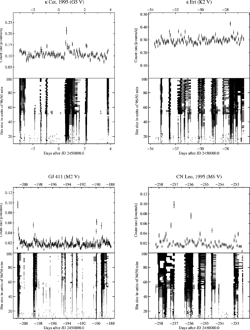
Figure 1: Examples of light curves and significance plots.

Figure 2: Cumulative flare occurrence rate constructed for all twelve data sets.

Figure 3: Power-law index $\alpha$ vs. coronal luminosity $L_{\mathrm{X}}$.

Figure 4: Occurrence rates of flares with energies larger than $10^{32}$ ergs vs. coronal luminosity $L_{\mathrm{X}}$. Data group 1 corresponds to the rates derived from the fits to cumulative distributions, while data group 2 corresponds to the rates derived from the fits to differential distributions. The $\chi^{2}$ linear best-fits in the $\log-\log$ plane are shown as straight lines together with the analytical formulation. Crosses represent $L_{\mathrm{X}}$ values for these sources taken from the literature (see text).

Figure 5: Coronal luminosity $L_{\mathrm{X}}$ vs. bolometric luminosity $L_{\mathrm{bol}}$. The source identification numbers refer to Table EUV FLARE ACTIVITY IN LATE-TYPE STARS. The solid line represents the saturation level ($L_{\mathrm{X}}/L_{\mathrm{bol}}=10^{-3}$), while the dotted line is for $L_{\mathrm{X}}/L_{\mathrm{bol}}=10^{-4}$, and the dashed line for $L_{\mathrm{X}}/L_{\mathrm{bol}}=10^{-5}$.

Figure 6: Normalized occurrence rate of flares with energies larger than $10^{32}$ ergs vs. ratio $L_{\mathrm{X}}/L_{\mathrm{bol}}$  of the coronal luminosity and the bolometric luminosity. Data groups 1 and 2 are identical to Fig. EUV FLARE ACTIVITY IN LATE-TYPE STARS. The numbers are as in Fig. EUV FLARE ACTIVITY IN LATE-TYPE STARS. The dash-dotted lines are lines with slope 1. The dotted lines represent the saturation level ($L_{\mathrm{X}}=10^{-3}L_{\mathrm{bol}}$). Note that, for clarity, the $N(>E_{\mathrm{c}})$ of points 4 and 9 have been multiplied and divided by a factor of 1.5, respectively.

Figure 7: Normalized occurrence rate of flares with energies larger than $10^{32}$ ergs vs. normalized projected rotational velocity $v\sin i/(v\sin i)_{\mathrm{sat}}=x$ (spectral-type dependent). Data groups 1 and 2 are identical to Fig. EUV FLARE ACTIVITY IN LATE-TYPE STARS. “Saturation” fits of the form $1-\exp(-x/{\zeta}$) are plotted dot-dashed. Arrows indicate upper limits. Note that, for clarity, the $N(>E_{\mathrm{c}})$ of points 4 and 5 have been divided and multiplied by a factor of 1.5, respectively.

Figure 8: (Upper and middle panels) Normalized flare rate vs. Rossby number. Data groups and identifications are as in Fig. EUV FLARE ACTIVITY IN LATE-TYPE STARS. (Lower panel) Ratio $L_{\mathrm{X}}/L_{\mathrm{bol}}$ vs. the Rossby number for our sample. The solid line corresponds to the fit by Randich et al. (1996), while the dashed line refers to our best fit (see text).

Figure 9: X-radiated power $P_{F}$ from the detected flares vs. coronal luminosity $L_{\mathrm{X}}$. The solid line represents proportionality ($P_{F}=L_{\mathrm{X}}$), while the dashed line is for $P_{F}=0.1L_{\mathrm{X}}$.

References

- Arnaud (1996) Arnaud, K. A. 1996, in ASP Conf. Ser. 101, Astronomical Data Analysis Software and Systems V, ed. G. Jacoby & J. Barnes (San Francisco: ASP), 17
- Aschwanden et al. (2000) Aschwanden, M. J., Tarbell, T. D., Nightingale, R. W., Schrijver, C. J., Title, A., Kankelborg, C. C., Martens, P. C. H., & Warren, H. P. 2000, ApJ, in press
- Audard et al. (1999) Audard, M., Güdel, M., & Guinan, E. F. 1999, ApJ, 513, L53
- Baliunas et al. (1983) Baliunas, S. L., Vaughan, A. H., Hartmann, L. W., Middelkoop, F., Mihalas, D., Noyes, R. W., Preston, G. W., Frazer, J., & Lanning, H. 1983, ApJ, 275, 752
- Caillault & Helfand (1985) Caillault, J.-P., & Helfand, D. J. 1985, ApJ, 289, 279
- Collier Cameron et al. (1988) Collier Cameron, A., Bedford, D. K., Rucinski, S. M., Vilhu, O., & White, N. E. 1988, MNRAS, 231, 131
- Collura et al. (1988) Collura, A., Pasquini, L., & Schmitt, J. H. M. M. 1988, A&A, 205, 197
- Crawford et al. (1970) Crawford, D. F., Jauncey, D. L., & Murdoch, H. S. 1970, ApJ, 162, 405
- Crosby et al. (1993) Crosby, N. B., Aschwanden, M. J., & Dennis, B. R. 1993, Sol. Phys., 143, 275
- Delfosse et al. (1998) Delfosse, X., Forveille, T., Perrier, C., & Mayor, M. 1998, A&A, 331, 558
- Dempsey et al. (1993a) Dempsey, R. C., Linsky, J. L., Fleming, T. A., & Schmitt, J. H. M. M. 1993a, ApJS, 86, 599
- Dempsey et al. (1997) ———. 1997, ApJ, 478, 358
- Dempsey et al. (1993b) Dempsey, R. C., Linsky, J. L., Schmitt, J. H. M. M., & Fleming, T. A. 1993b, ApJ, 413, 333
- Doyle & Butler (1985) Doyle, J. G., & Butler, C. J. 1985, Nature, 313, 378
- Drake et al. (2000) Drake, J. J., Kashyap, V. L., Audard, M., & Güdel, M. 2000, ApJ, in preparation
- Fekel (1997) Fekel, F. C. 1997, PASP, 109, 514
- Feldman et al. (1995) Feldman, U., Laming, J. M., & Doschek, G. A. 1995, ApJ, 471, L79
- Gehrels (1986) Gehrels, N. 1986, ApJ, 303, 336
- Gliese & Jahreiss (1991) Gliese, W., & Jahreiss, H. 1991, Preliminary version of the Third Catalogue of Nearby Stars, on: The Astronomical Data Center CD-ROM: Selected Astronomical Catalogues, Vol. 1; ed. L. E. Brotzmann & S. E. Gesser, NASA/Astronomical Data Center, Goddard Space Flight Center, Greenbelt, MD
- Groot et al. (1996) Groot, P. J., Piters, A. J. M., & van Paradijs, J. 1996, A&AS, 118, 545
- Güdel (1994) Güdel, M. 1994, ApJS, 90, 743
- Güdel et al. (1997) Güdel, M., Guinan, E. F., & Skinner, S. L. 1997, ApJ, 483, 947
- Güdel et al. (1995) Güdel, M., Schmitt, J. H. M. M., & Benz, A. O. 1995, A&A, 293, L49
- Güdel et al. (2000) Güdel, M., et al. 2000, ApJ, in preparation
- Haisch & Schmitt (1996) Haisch, B., & Schmitt, J. H. M. M. 1996, PASP, 108, 113
- Hearn (1975) Hearn, A. G. 1975, A&A, 40, 355
- Hudson (1991) Hudson, H. S. 1991, Sol. Phys., 133, 357
- Hünsch et al. (1999) Hünsch, M., Schmitt, J. H. M. M., Sterzik, M. F., & Voges, W. 1999, A&AS, 135, 319
- Hünsch, Schmitt, & Voges (1998) Hünsch, M., Schmitt, J. H. M. M., & Voges, W. 1998, A&AS, 132, 155
- Innis et al. (1988) Innis, J. L., Thompson, K., Coates, D. W., & Lloyd Evans, T. 1988, MNRAS, 235, 1411
- Ionson (1985) Ionson, J. A. 1985, Sol. Phys., 100, 289
- Jordan & Montesinos (1991) Jordan, C., & Montesinos, B. 1991, MNRAS, 252, 21
- Jordan et al. (1987) Jordan, C., Ayres, T. R., Brown, A., Linsky, J. L., & Simon, T. 1987, MNRAS, 225, 903
- Kaastra et al. (1996) Kaastra, J. S., Mewe, R., & Nieuwenhuijzen H. 1996, in UV and X-ray Spectroscopy of Astrophysical and Laboratory Plasmas, ed. K. Yamashita & T. Watanabe, (Tokyo: Univ. Acad. Press), 411
- Kopp & Poletto (1993) Kopp, R. A., & Poletto, G. 1993, ApJ, 418, 496
- Kraft (1967) Kraft, R. P. 1967, ApJ, 150, 551
- Krucker & Benz (1998) Krucker, S., & Benz, A. O. 1998, ApJ, 501, L213
- Kürster et al. (1994) Kürster, M., Schmitt, J. H. M. M., & Cutispoto, G. 1994, A&A, 289, 899
- Jakimiec et al. (1992) Jakimiec, J., Sylwester, B., Sylwester, J., Serio, S., Peres, G., & Reale, G. 1992, A&A, 253, 269
- Linsky (1985) Linsky, J. L. 1985, Sol. Phys., 100, 333
- Linsky & Gary (1983) Linsky, J. L., & Gary, D. E. 1983, ApJ, 274, 776
- Linsky & Wood (1994) Linsky, J. L., & Wood, B. E. 1994, ApJ, 430, 342
- Malina & Bowyer (1991) Malina, R. F., & Bowyer, S. 1991, in Extreme-Ultraviolet Astronomy, ed. R. F. Malina & S. Bowyer, (New York: Pergamon), 391
- Monsignori Fossi et al. (1996) Monsignori Fossi, B. C., Landini, M., Del Zanna, G., & Bowyer, S. 1996, ApJ, 466, 427
- Narain & Ulmschneider (1990) Narain, U., & Ulmschneider, P. 1990, Space Sci. Rev., 54, 377
- Noyes et al. (1984) Noyes, R. W., Hartmann, L. W., Baliunas, S. L., Duncan, D. K., & Vaughan, A. H. 1984, ApJ, 279, 763
- Osten & Brown (1999) Osten, R. A., & Brown, A. 1999, ApJ, 515, 746
- Pallavicini et al. (1981) Pallavicini, R., Golub, L., Rosner, R., Vaiana, G. S., Ayres, T., & Linsky, J. L. 1981, ApJ, 248, 279
- Pallavicini et al. (1988) Pallavicini, R., Monsignori-Fossi, B. C., Landini, M., & Schmitt, J. H. M. M. 1988, A&A, 191, 109
- Pallavicini et al. (1990) Pallavicini, R., Tagliaferri, G., & Stella, L. 1990, A&A, 228, 403
- Parker (1988) Parker, E. N. 1988, ApJ, 330, 474
- Parnell & Jupp (2000) Parnell, C. E., & Jupp, P. E. 2000, ApJ, 529, 554
- Perryman et al. (1997) Perryman, M. A. C., Lindegren, L., Kovalevsky, J., et al. 1997, A&A, 323, L49
- Pettersen et al. (1992) Pettersen, B. R., Olah, K., & Sandmann, W. H. 1992, A&AS, 96, 497
- Porter et al. (1995) Porter, J. G., Fontenla, J. M., & Simnett, G. M. 1995, ApJ, 438, 472
- Press et al. (1992) Press, W. H., Teukolsky, S. A., Vetterling, W. T., & Flannery, B. P. 1992, Numerical Recipes in Fortran 77: the art of scientific computing – 2nd ed., (Cambridge: CUP), 637
- Randich et al. (1996) Randich, S., Schmitt, J. H. M. M., Prosser, C. F., & Stauffer, J. R. 1996, A&A, 305, 785
- Robinson et al. (1999) Robinson, R. D., Carpenter, K. G., & Percival, J. W. 1999, ApJ, 516, 916
- Robinson et al. (1995) Robinson, R. D., Carpenter, K. G., Percival, J. W., & Bookbinder, J. A. 1995, ApJ, 451, 795
- Rosner et al. (1978) Rosner, R., Tucker, W. H., & Vaiana, G. S. 1978, ApJ, 220, 643
- Schmidt-Kaler (1982) Schmidt-Kaler, T. H. 1982, In Landolt-Börnstein New Series, Vol. 2B, Astronomy & Astrophysics – stars and star clusters, ed. K. Schaifers & H. H. Voigt, (Berlin: Springer), 15 & 453
- Schmitt et al. (1995) Schmitt, J. H. M. M, Fleming, T. A., & Giampapa, M. S. 1995, ApJ, 450, 392
- Schrijver et al. (1984) Schrijver, C. J., Mewe, R., & Walter, F. M. 1984, A&A, 138, 258
- Sciortino et al. (1999) Sciortino, S., Maggio, A., Favata, F., & Orlando, S. 1999, A&A, 342, 502
- Shimizu (1995) Shimizu, T. 1995, PASJ, 47, 251
- Simon (2000) Simon, T. 2000, In Eleventh Cambridge Workshop on Cool stars, Stellar Systems, and the Sun, ed. R. J. García López, R. Rebolo, & M. R. Zapatero Osorio (San Francisco:ASP), in press
- Skumanich (1972) Skumanich, A. 1972, ApJ, 171, 565
- Skumanich (1985) Skumanich, A. 1985, Aust. J. Phys., 38, 971
- Spiesman & Hawley (1986) Spiesman, W. J., & Hawley, S. L. 1986, ApJ, 92, 664
- Stauffer et al. (1994) Stauffer, J. R., Caillault, J.-P., Gagné, M., Prosser, C. F., & Hartmann, L. W. 1994, ApJS, 91, 625
- Stauffer et al. (1997) Stauffer, J. R., Hartmann, L. W., Prosser, C. F., Randich, S., Balachandran, S., Patten, B. M., Simon, T., & Giampapa, M. 1997, ApJ, 479, 776
- Strassmeier & Rice (1998) Strassmeier, K. G., & Rice, J. B. 1998, A&A, 330, 685
- Strassmeier et al. (1997) Strassmeier, K. G., Bartus, J., Cutispoto, G., & Rodonò, M. 1997, A&AS, 125, 11
- Stȩpień (1993) Stȩpień, K. 1993, in The Cosmic Dynamo, ed. F. Krause, K.-H. Rädler, & G. Rüdiger, (Dordrecht: Kluwer), 141
- Tagliaferri et al. (1997) Tagliaferri, G., Covino, S., Fleming, T. A., Gagné, M., Pallavicini, R., Haardt, F., & Uchida, Y. 1997, A&A, 321, 850
- Vaiana et al. (1981) Vaiana, G. S., et al. 1981, ApJ, 245, 163
- van den Oord et al. (1988) van den Oord, G. H. J., Mewe, R., & Brinkman, A. C. 1988, A&A, 205, 181
- Vilhu (1984) Vilhu, O. 1984, A&A, 133, 117
- Vilhu & Walter (1987) Vilhu, O., & Walter, F. M. 1987, ApJ, 321, 958
- Walter (1981) Walter, F. M. 1981, ApJ, 245, 677
- Walter (1982) ———. 1982, ApJ, 253, 745
- Walter & Bowyer (1981) Walter, F. M., & Bowyer, S. 1981, ApJ, 245, 671
- Wood et al. (1996) Wood, B. E., Harper, G. M., Linsky, J. L., & Dempsey, R. C. 1996, ApJ, 458, 761
- Zirker (1993) Zirker, J. B. 1993, Sol. Phys., 148, 43