Theoretical Predictions for Surface Brightness Fluctuations
and Implications for Stellar Populations of Elliptical Galaxies
Abstract
We compute theoretical predictions for surface brightness fluctuations (SBFs) of single-burst stellar populations (SSPs) using models optimized for this purpose. We present results over a wide range of ages (from 1 to 17 Gyr) and metallicities (from 1/200 to 2.5 times solar) and for a comprehensive set of ground-based and space-based optical and infrared bandpasses. Our models agree well with existing SBF observations of Milky Way globular clusters and elliptical galaxies.
Our results provide refined theoretical calibrations and -corrections that are needed to use SBFs as standard candles. We suggest that SBF distance measurements can be improved by (1) using a filter around 1 µm to minimize the influence of stellar population variations, and (2) using the integrated galaxy color instead of to calibrate -band SBF distances.
We show that available SBF observations set useful constraints on current population synthesis models, and we suggest SBF-based tests for future models. The existing SBF data favor particular choices of stellar evolutionary tracks and spectral libraries among the several choices allowed by comparisons based on only the integrated properties of galaxies. Also, the tightness of the empirical -band SBF calibration as a function of galaxy color is a useful constraint. It suggests that the model uncertainties in the lifetimes of the post-main sequence evolutionary phases are probably less than 50% and that the initial mass function in elliptical galaxies is probably not much steeper than that in the solar neighborhood.
Finally, we analyze the potential of SBFs for probing unresolved stellar populations in elliptical galaxies. Since SBFs depend on the second moment of the stellar luminosity function, they are sensitive to the brightest giant stars and provide complementary information to commonly-used integrated light and spectra. In particular, we find that optical/near-infrared SBFs are much more sensitive to the metallicity than the age of a stellar population. Therefore, in combination with age-sensitive observables, SBF magnitudes and colors are a valuable complement to metal-line indices to break the age/metallicity degeneracy in elliptical galaxy studies. Our preliminary results suggest that the most luminous stellar populations of bright galaxies in nearby clusters have roughly solar metallicites and about a factor of three spread in age.
1 Introduction
When observing the inner regions of a nearby elliptical galaxy or the bulge of a nearby spiral galaxy, there are two noticeable characteristics of the surface brightness structure of these spheroidal stellar systems. The first characteristic is that the galaxy is brightest in the center with the surface brightness falling off gradually with increasing radial distance. The second characteristic is only apparent in good seeing conditions: on small scales, the galaxy has a clumpy appearance on the spatial scale of the seeing disk. The clumpiness arises from Poisson statistical variations in the number of stars within each resolution element. This effect can be easily recognized by visual inspection of images of nearby galaxies like M 31 and M 32, in which the small-scale clumpiness can be a few percent of the mean surface brightness. Historically, this effect was called “incipient resolution.” In the modern context, it is known as surface brightness fluctuations (SBFs).
Tonry & Schneider (1988) devised a technique to quantify SBFs for use as an extragalactic distance indicator for undisturbed early-type galaxies. (See also the reviews by Jacoby et al., 1992 and Blakeslee et al., 1999.) This method relies on using the ratio of the second moment to the first moment of the stellar luminosity function (LF) of the galaxy as a standard candle:
| (1) |
where is the number of stars of type and luminosity . The quantity has units of luminosity and is referred to as when represented as an absolute magnitude. The apparent SBF magnitude can be determined observationally, and if the distance to the galaxy is known, can also be determined. Of course, as in the case of ordinary photometry, SBF colors are distance-independent (provided that the -correction is negligible). Using SBFs as a distance indicator requires that (1) the bright end of the stellar LF in elliptical galaxies and spiral bulges is universal, or (2) variations in the LF from galaxy to galaxy can be measured and corrected so that remains a standard candle.
SBFs are an intrinsic property of a stellar population as a whole. Therefore, in addition to their utility as a distance indicator, SBFs offer much promise in adding to our knowledge of the stellar content of elliptical galaxies. In fact, the use of SBFs for stellar population studies arguably preceded its use as a distance indicator: Baum & Schwarzschild (1955) used the ”count-brightness ratio,” the ratio of the number of resolved stars to the integrated light, to study the populations of M 31 and M 32. Hence, the idea of using observations near or at the limit of resolution to explore stellar populations has a long history.
Furthermore, SBFs provide information about stellar populations unique from ordinary integrated light, which is the first moment of the stellar LF. Since SBFs also depend on the second moment of the stellar luminosity function, they are especially sensitive to the most luminous stars in elliptical galaxies, the evolved cool giant stars. Thus, SBFs can put stronger constraints on the evolution of these stars than integrated light alone. Both the interior structure and emergent spectral energy distributions of cool giant stars are poorly understood, especially near the tip of the red giant branch (RGB) and the asymptotic giant branch (AGB) populated by low and intermediate mass () stars. Ideally, we would study these stars using Local Group star clusters, which comprise populations of homogenous composition and age. However, because cool giants evolve rapidly, only a handful are present in any cluster; therefore, small number statistics and stochastic fluctuations are undesireable factors (e.g., Santos & Frogel, 1997). In this context, SBF analyses of entire galaxies can complement star cluster studies, since galaxian light arises from several orders of magnitude more stars. Also, while nearby globular clusters are mostly metal-poor, the dominant stellar populations in ellipticals are thought to be generally old and metal-rich. There is a dearth of such systems in the Local Group — the best examples are the bulges of the Milky Way and M 31, but these may be imperfect analogs. In order to study metal-rich stellar evolution, one naturally turns to elliptical galaxies.
There are two basic motivations for modeling SBFs: (1) as pointed out by Tonry & Schneider (1988), one can derive the calibration of SBF absolute magnitudes purely from models provided that stellar populations in galaxies can be modeled accurately, and alternatively, (2) one can use the observations of SBF magnitudes and colors to test and improve the models.
The first attempt at deriving a purely theoretical SBF zeropoint was that of Tonry et al. (1990). They used stellar evolutionary models from the Revised Yale Isochrones (Green et al., 1987, hereinafter RYI) supplemented with simple prescriptions for the horizontal branch and AGB; the resulting zeropoint and especially its dependence on the integrated galaxy color disagreed significantly with observations (Tonry, 1991). This was due to the fact that the RYI giant branches failed to turn over in the optical at high metallicity, probably because of inaccurate bolometric corrections for the coolest giant stars (Mould, 1992; Ajhar & Tonry, 1994). A subsequent study was made by Worthey (1993a), who computed SBF magnitudes using his own population synthesis models (Worthey, 1994). For the main-sequence and RGB stars, these models used an amalgamation of isochrones from Vandenberg and collaborators with the RYI; post-RGB evolution was added using the fuel consumption theorem, including “schematic” treatments of the HB as a single red clump and of AGB evolution using a variety of theoretical prescriptions. The resulting SBF predictions agreed well with the observed optical SBF colors (, , and ) and with the empirical calibration of versus (see also Tonry et al., 1997). Buzzoni (1993) also computed predictions for SBF magnitudes which were consistent with the existing optical SBF data at the time, though there were some uncertainties in transforming from the Johnson filters used in his models to the Kron-Cousins ones used for the observations. Since his models used older theoretical spectra (Bell & Gustafsson, 1978), Buzzoni had to extrapolate the spectra for wavelengths longward of 1.08 µm and also for stars with K. For both of these reasons, the Buzzoni (1993) models are expected to be less accurate for SBF predictions in the IR. For example, their predictions are at least several tenths of a magnitude fainter in the -band than the observations.
The major observational effort on SBFs has been focused on -band measurements for distance determinations. As mentioned above, comparisons of stellar population models with observed SBF magnitudes and colors can also help us calibrate the colors (i.e., stellar spectral energy distributions [SEDs]) and numbers (i.e., evolutionary lifetimes) of cool luminous giant stars in old stellar populations. SBF stellar population studies have been less explored than distance measurements, partly because of the lack of suitable datasets. Multicolor optical () SBF measurements for Virgo cluster galaxies from Tonry et al. (1990) were analyzed by both Worthey (1993a) and Buzzoni (1993), who reached opposite conclusions on whether the optical SBF colors indicated that the galaxies contained a significant metal-poor component. Ajhar & Tonry (1994) measured -band SBFs for a sample of Galactic globular clusters, the only observations to date for these systems. They sought to understand the empirical -band SBF zeropoint and its correlation with integrated galaxy colors, as well as the conflict between the data and the RYI models; they also addressed the use of optical SBF colors for stellar population studies in galaxies and for disentangling age from metallicity effects in globular clusters. Sodemann & Thomsen (1995, 1996) performed a detailed study of the optical SBF gradients within the nearby ellipticals M 32 and NGC 3379. Finally, Jensen et al. (1998) found reasonable agreement between their -band SBF data for 11 nearby galaxies and the Worthey (1993a) models, with most of the galaxies lying around the [Fe/H] = –0.25 models with a spread in ages.
Now is a ripe opportunity to revisit the issue of stellar population modeling of surface brightness fluctuations. There have been significant recent improvements in the stellar evolution calculations and spectral libraries used by population synthesis models. For example, the latest stellar evolution calculations include updated input radiative opacities (e.g., Iglesias et al., 1992). There has been even more progress on the observational front. The amount of -band SBF data has increased by nearly tenfold since the early modeling of Worthey (1993a), and new data in the near-infrared have extended the spectral range of SBF measurements (Pahre & Mould, 1994; Jensen et al., 1998; Liu et al., 2000; Mei et al., 2000).
In this paper, we present new models for optical/infrared SBFs of intermediate-age and old single-burst stellar populations (SSPs) and discuss their implications for SBF distance measurements and stellar population studies. Though interesting issues remain to be addressed by blue/near-UV SBF measurements (Worthey, 1993b), we focus on the optical and near-infrared (i.e., -band to -band) SBFs, since these constitute the bulk of past and ongoing observations. In § 2, we describe our models for computing SBFs. The models cover a wider range of ages and metallicities than in previous SBF studies. Furthermore, we have optimized the models for this work by refining the prescription for the luminous cool stars, which are important contributors to the SBF signal. In § 3, we present the predictions of our models, including SBF magnitudes, integrated colors, and the fractional contribution of different stellar evolutionary phases to the SBFs. We also derive theoretical calibrations and -corrections that are needed to use SBFs standard candles. In § 4, we compare our results with current SBF observations and discuss implications for the stellar content of elliptical galaxies. In § 5, we review the uncertainties in our results and explore the potential of SBFs for breaking the age-metallicity degeneracy in studies of elliptical galaxies. Finally in § 6, we summarize our findings and offer some future directions for SBF studies.
2 Synthesizing SBFs of Stellar Populations
In this section, we present our models for computing SBFs. We first recall the origin of the SBF signal of stellar populations. We then review current observations of the stars which dominate this signal in order to establish a framework to interpret the model results. Readers interested only in the description of our models should skip to § 2.3.
2.1 Origin of the SBF Signal
Since SBFs are weighted by the square of the stellar luminosity, they are very sensitive probes of the most luminous cool giant stars. For example, for the idealized case of a stellar population with a simple power-law luminosity function, one can easily show via equation (1) that the fluctuation luminosity scales linearly with the maximum luminosity of the stars. Figure 1 illustrates the greater sensitivity to luminous giant stars of SBFs compared to ordinary integrated light for a more realistic model stellar population (see § 2.3 below). For this 12 Gyr solar-metallicity model, about 90% of the SBF signal is contributed by the brightest 2 mags of the stellar luminosity function in the near-IR and the brightest 3–5 mags in the optical. Clearly, the optical/infrared SBF signal is heavily weighted to the very brightest stars in a stellar population.
2.2 Observed Properties of Cool Giant Stars
Since SBF magnitudes and colors are expected to closely follow the peak magnitude and colors of the giant branch, it is insightful to review the observed properties of cool giant stars, both on the RGB (H-shell burning) and the AGB (He-shell burning), as a function of age and metallicity for Milky Way and Magellanic Cloud star clusters.
2.2.1 Giant Branches of Old Stellar Populations
The colors of the giant branches of old (5 Gyr) stellar populations are primarily driven by metallicity, with more metal-rich systems having redder giant branch colors (e.g., Frogel et al., 1983). This is illustrated in Figure 2, which shows the change in the temperature of the RGB and AGB for a change in metallicity from [Fe/H] = –0.7 to +0.4 with ages of 5 and 12 Gyr. This trend results from the increase in opacity with metallicity from H- ions, which are the principal source of continuum opacity for stars with K. Metals with low-ionization potential are the primary electron donors. Thus, as the metallicity increases, H- opacity increases and the giant branch temperature drops. It is interesting to note that since Mg and Si are also significant donors along with Fe (Renzini, 1977), the giant branch color traces the total metallicity [Z/H] and not just the Fe abundance [Fe/H] (e.g., Geisler, 1984; see discussion in Salaris & Cassisi, 1996). In stellar evolution models, the absolute temperature of the RGB depends on the choice of the mixing length used to parameterize the interior convection (e.g., Renzini & Fusi Pecci, 1988).
Similarly, the shape of the RGB, as measured from the RGB slope in optical/IR color-magnitude diagrams, is also primarily driven by the metal abundance for old populations, with more metal-rich clusters having steeper slopes (Kuchinski et al., 1995; Kuchinski & Frogel, 1995; Tiede et al., 1997; Ferraro et al., 1999). This implies that giant stars which contribute to the SBF signal will have a larger spread in color for metal-rich populations than metal-poor ones.
The tip of the RGB (TRGB) is delineated by core-He ignition. The TRGB bolometric luminosity in Milky Way globular clusters increases modestly with metallicity (Frogel et al., 1981, 1983).111Observations actually measure the brightest RGB stars in the clusters, rather than the true tip of the RGB. Therefore, there is a potential systematic underestimate of the tip luminosity due to statistical sampling. Unpublished estimates by Rood & Crocker (1997) show that this effect is probably not significant for the Frogel et al. data (see also Ferraro et al., 1999). The optical and IR magnitudes for the TRGB have opposite dependences on metallicity. In the optical, increasing metallicity leads to increased opacity from molecular lines, especially from TiO, which reduces the optical flux. Hence, the TRGB in the optical becomes cooler and fainter as metallicity increases, first turning over in the -band and then also in the -band for the most metal-rich Milky Way globular clusters (e.g., Lloyd Evans & Menzies, 1977; Da Costa & Armandroff, 1990; Ortolani et al., 1991; Bica et al., 1991). Thus the brightest stars of metal-rich globular clusters are fainter in the optical than those of metal-poor clusters. On the other hand, in the near-IR the -band magnitude of the TRGB of Milky Way globular clusters rises monotonically with metallicity, with a roughly 1 mag increase over the range (Ferraro et al., 1999).
The AGB is expected to follow the behavior of the RGB in old populations and reach cooler temperatures with increasing metal abundance. AGB studies in globular clusters are hampered by the scarcity of stars found in this short evolutionary stage in any given cluster. The AGB is usually divided into two phases: (1) the initial early AGB (E-AGB), where He-shell burning proceeds steadily, and (2) the thermally pulsing AGB (TP-AGB), characterized by oscillations in luminosity due to periodic flashes of the He shell. Mass loss is believed to occur during both of these phases and to end in a superwind stage. In metal-poor ([Fe/H] ) Milky Way globular clusters, the luminosities of the brightest AGB stars do not exceed the tip of the RGB. In more metal-rich systems, long-period variables are observed above the tip of the RGB, which are presumably TP-AGB stars (Frogel & Elias, 1988). In fact, since AGB stars follow a core mass-luminosity relation (Paczynski, 1971) and the main-sequence turnoff mass increases with metallicity at a fixed age (Renzini & Fusi Pecci, 1988), higher metallicity leads to brighter AGB stars.
2.2.2 Extended Giant Branches of Intermediate-Age Populations
Information on intermediate-age ( Gyr) stellar populations largely comes from studies of star clusters in the Large and Small Magellanic Clouds (LMC/SMC). The brightest stars in these clusters are carbon AGB stars with bolometric magnitudes much brighter than the tip of the RGB (Mould & Aaronson, 1979; Frogel et al., 1980; Mould & Aaronson, 1980; Cohen et al., 1981). These very cool stars provide a significant fraction of the total luminosity of the clusters (Persson et al., 1983). They are redder and more luminous than the M-type AGB stars. In contrast, the brightest stars in old LMC/SMC clusters are M giants no brighter than the brightest stars in Galactic globular clusters (Aaronson & Mould, 1985; Frogel et al., 1990; Marigo et al., 1996). As a result, the near-IR colors of intermediate-age clusters (types IV to VI of Searle et al., 1980) are much redder than those of older or younger clusters, whereas the optical colors redden monotonically with cluster age.
Carbon stars are believed to arise from carbon dredge-up during the TP-AGB phase (Iben & Renzini, 1983). The observed ratio of C-stars to M-stars in Local Group galaxies anti-correlates with metallicity, C-stars being the dominant spectral type for [Fe/H] (Blanco et al., 1978; Cook et al., 1986; Pritchet et al., 1987). This occurs because stars with lower metallicities require fewer thermal pulses to change from an O-rich to a C-rich star. In addition, dredge-up is more efficient at lower metallicities because it begins at lower core masses, i.e., at earlier ages. There are no examples of solar-metallicity intermediate-age clusters in the LMC/SMC which would be most directly comparable to elliptical galaxies. However, models by Vassiliadis & Wood (1993) predict that the bolometric luminosity of the tip of the AGB should remain much brighter than the tip of the RGB and have even cooler temperatures and redder colors than in LMC/SMC clusters (see also discussion in Silva & Bothun, 1998).
Since the giant branches of intermediate-age Magellanic Cloud clusters reach higher luminosities than those of old Galactic clusters, they are often referred to as “extended” giant branches and are considered the hallmark of intermediate-age populations (e.g., Guarnieri et al., 1997). This occurs because the core mass-luminosity relation for AGB stars implies that younger populations have more luminous AGB stars. In the context of SBF studies, elliptical galaxies are generally thought to be composed entirely of old stellar populations. However, any recent episodes of star formation would lead to extended giant branches. The observable consequence of this would be brighter fluctuation magnitudes (and perhaps somewhat redder fluctuation colors), especially in the infrared, without significant changes in the integrated colors of the galaxies.222Extended giant branches have been claimed to be detected in optical and near-IR images of M 32 and the bulge of M 31 (Rich & Mould, 1991; Freedman, 1992; Elston & Silva, 1992; Rich et al., 1993), which would mean recent star formation in these supposedly canonical examples of old stellar populations. However, more recent work has suggested this conclusion is erroneous and due to severe image crowding (Depoy et al., 1993; Grillmair et al., 1996; Renzini, 1998; Sodemann & Thomsen, 1998; Jablonka et al., 1999). In addition, as pointed out by Renzini (1998), the presence of objects brighter than the tip of the RGB ( for solar-metallicity) cannot be readily interpreted as the sign of an intermediate-age population. Long-period variables in metal-rich globular clusters do reach , so the only unambiguous signs of an intermediate-age population would be either the presence of (1) stars with even larger bolometric luminosities or (2) many more stars with to 5 than expected in a metal-rich population. We return to this point in § 4.3 and § 6.
2.3 Stellar Population Synthesis Models for SBFs
We use the latest version of the Bruzual-Charlot population synthesis models (Bruzual & Charlot, 2000, hereinafter BC2000). These models allow us to predict the spectral evolution of stellar populations with arbitrary star formation rates and initial mass functions (IMFs) for a wide range of metallicities. The main ingredients of the models are the stellar evolution theory used to predict the distribution of stars in the theoretical Hertzsprung-Russell diagram and the library of spectra assigned to stars as a function of effective temperature and luminosity. The integrated spectrophotometric properties of an entire stellar population are obtained by summing the spectra of its component stars. We now describe the model features most relevant to the present work.
2.3.1 Model Inputs
The BC2000 models present several major improvements over the earlier models of Bruzual & Charlot (1993). They also offer several choices of input stellar evolution theory and atmospheres (Table 1). Stellar evolution can be followed according to the prescription of the Geneva school for solar metallicity or that of the Padova school for metallicites ranging from 1/200 to 2.5 times solar. (See Charlot et al., 1996 for a detailed description of the two prescriptions, and Bruzual et al., 1997 for a complete list of references.) These prescriptions include all phases of stellar evolution from the zero-age main sequence to the beginning of the TP-AGB (for low- and intermediate-mass stars) and core-carbon ignition (for massive stars). In both sets of tracks, solar metallicity corresponds to , and in the Padova tracks, the metallicity scales as [Fe/H] = 1.024 log + 1.739 (Bertelli et al., 1994). We note that the Padova and Geneva models predict very different fractional contributions from RGB and AGB stars to the integrated light of solar-metallicity SSPs (Bruzual, 1996); this has strong implications for SBF predictions.333Girardi et al. (2000) have recently updated the Padova library. The new library covers only a limited range of initial stellar masses and metallicities and cannot be combined with the library used here because of the slightly different chemical composition used at a fixed metallicity. The new tracks are almost identical to the previous ones, the main purpose of the new library being a finer sampling of initial stellar masses (Girardi et al. 2000; A. Bressan 2000, private communication).
Bruzual & Charlot (2000) supplemented these tracks with a new prescription for the thermally-pulsing regime at the tip of the AGB, which improves over that adopted by Bruzual & Charlot (1993). This prescription was motivated by the inability of that proposed by Charlot & Bruzual (1991) to account for the SBF properties of observed galaxies when we started the present study.444Preliminary results for the -band SBF magnitudes in Liu et al. (1999a, b) used the old TP-AGB prescription and are supplanted by the results in this paper. In the new prescription, the effective temperatures, bolometric luminosities, and lifetimes (of both the optically-visible and superwind phases) of TP-AGB stars of various metallicities are taken from the models of Vassiliadis & Wood (1993). For stars undergoing a transition from oxygen-rich (M-type) to carbon-rich (C-type) on the TP-AGB, the relative lifetimes of the two phases as a function of metallicity are taken from the models of Groenewegen & de Jong (1993) and Groenewegen et al. (1995). These models reproduce the observed ratios of C to M stars in the LMC and the Galaxy; however, since they do not extend to sub-Magellanic () nor super-solar () metallicities, the same relative durations of the M-type and C-type phases are applied to the Padova tracks at the more extreme metallicities. Finally, the tracks are supplemented with a prescription for post-AGB evolution and with unevolving main-sequence stars in the mass range 0.1–0.6 .
The BC2000 models also offer a choice of spectral libraries, summarized in Table 1. For solar metallicity, a quasi-empirical set of spectra is available from a compilation by Pickles (1998). The spectra of M0–M10 giant stars are the only non-empirical ones in this library, as they are based on the synthetic M-giant spectra computed by Fluks et al. (1994). These models were constructed to reproduce period-averaged spectra from observations of long-period variable TP-AGB stars. In the remainder of this paper, we refer to this spectral library as the empirical SEDs.
For stars of all metallicities, a comprehensive spectral library has been assembled by Lejeune et al. (1997, 1998, hereinafter LCB97). It is a combination of model atmospheres by Kurucz (1995; private communication to Lejeune), Bessell et al. (1989, 1991), and the same Fluks et al. (1994) spectra as above, rebinned onto homogeneous scales in wavelength and physical parameters (effective temperature, surface gravity, and metallicity). Hereinafter, we refer to this spectral library as the theoretical SEDs.
LCB97 further corrected the synthetic spectra in their library by requiring that these reproduce the color-temperature relations observed for solar-metallicity stars (see also Lejeune et al., 1996). This adjustment is especially important for the M-star spectra. Lacking empirical calibration for non-solar metallicities, LCB97 applied the corrections derived at solar metallicities to all other metallicities. We refer to this spectral library as the semi-empirical SEDs.
Bruzual & Charlot (2000) supplemented all three of these spectral libraries with period-averaged spectra for C-type stars on the TP-AGB based on model atmospheres from Loidl et al. (1999, private communication; see Höfner et al., 2000). BC2000 applied empirical corrections to these spectra to match observed color-color calibrations by Mendoza & Johnson (1965). The spectra of stars in the superwind phase at the end of the TP-AGB are based on observations by Le Sidaner & Le Bertre (1996) and Le Bertre (1997, and references therein).
The models used here have been tested successfully against observed spectra of star clusters and galaxies (Bruzual et al., 1997; Bruzual & Charlot, 2000). Complementary descriptions and applications of previous versions of these models can also be found in Charlot et al. (1996), Bruzual et al. (1997), and Kauffmann & Charlot (1998). Bruzual (1996) has compared the results of different population synthesis codes and examined the dependence of integrated galaxy colors, SEDs, and spectral indices predicted by the Bruzual & Charlot (1998) models (very similar to BC2000 for his purposes) on the choice of input evolutionary tracks and spectra.
Unless otherwise indicated, in all calculations below we adopt a Salpeter (1955) IMF truncated at 0.1 and 125 . For old (5 Gyr) populations, adopting the Scalo (1986) IMF would lead to fluctuation magnitudes only 0.05 mag brighter and integrated colors only 0.02 mag bluer. (The changes are somewhat larger at younger ages; at 1 Gyr, the Scalo IMF leads to ’s fainter by about 0.1–0.2 mag.) These changes would have a negligible effect on our results and the agreement of our models with SBF observations. (See § 5.2 for a discussion of alternative IMFs.) Furthermore, in this paper, we approximate star clusters and elliptical galaxies as single-burst stellar populations. While this approximation is adequate for our present purposes, it limits investigations of the star formation history of elliptical galaxies. This is our goal in a complementary study (M. Liu et al., in preparation; see also § 6).
2.3.2 Model Outputs
We compute SBF magnitudes of single-burst stellar populations for ages of 1–17 Gyr and metallicities (, [Fe/H] = –2.4 to +0.4). We generate results for the bandpasses used by ground-based observatories and the and bandpasses used by the WFPC2 and NICMOS instruments aboard HST. The zeropoints for our magnitudes are computed on the Vega magnitude system.
The response functions for the Johnson-Morgan bandpasses are from Buser (1978). The and bandpasses are from Bessell (1990). For the ground-based near-infrared bandpasses, we use traces from Bessell & Brett (1988).555There is potential ambiguity in the notation of and . In the case of , this can be either the fluctuation luminosity or the SBF magnitude in the -band filter ( µm); we discuss the filter only in § 5.3 and Table 2. In the case of , we use this to refer generically to the SBF absolute magnitude in any filter bandpass. This could also represent the SBF absolute magnitude in the -band filter (), but we avoid using this representation except in Table 2. These are similiar to the filter system used at the UK Infrared Telescope (UKIRT), which is described in Leggett (1992) and Casali & Hawarden (1992). We choose not to use the CIT bandpasses (Elias et al., 1982) as the effective wavelength of the CIT -band is noticeably redder than that of most other IR systems (e.g., Leggett, 1992; Bessell & Brett, 1988) due to a Si lens in the original CIT dewar which defined the blue end of the bandpass.
We also include calculations for popular alternatives to the filter: the (1.9–2.3 micron; Wainscoat & Cowie, 1992) and (2.0–2.3 µm; McLeod et al., 1995) bandpasses. The filter trace is from the IR imager CIRIM used at Cerro Tololo Interamerican Observatory, and the filter is from the UCLA Gemini instrument at Lick Observatory (McLean et al., 1994). Our filter is virtually identical to that in the Hawaii QUIRC infrared camera (Hodapp et al., 1996) used by Jensen et al. (1998, 1999) for their SBF measurements. However, it is slightly different than the trace originally given by Wainscoat & Cowie (1992) in that the peak transmission of our filter is slightly redder. Transmission data for these IR filters were measured at 77 K. The traces were then multiplied with a theoretical model for atmospheric transmission generated by the ATRAN program (Lord, 1992) as atmospheric absorption can be significant at the edges of the bandpasses. We also included the (negligible) effect of the quantum efficiency (QE) of the IR detectors in these bandpasses.
The HST bandpasses include the filter transmission profiles, the spectral response of the HST mirror and instrument optics, and the QE of the detectors. The latter is especially important for the NICMOS filters as the QE rises sharply from 1–2 µm (MacKenty et al., 1997) due to the low operating temperature of the instrument’s HgCdTe arrays.
Also, we compute the ordinary , , and integrated colors of the SSPs and the strengths of several absorption lines (, Mg2, Mgb, H, and C4668) defined on the standard Lick/IDS system (Worthey, 1994; Worthey et al., 1994; Worthey & Ottaviani, 1997). We use the analytic fitting functions derived in these studies for index strength as a function of stellar temperature, gravity, and metallicity. We note that -element enhancement in massive elliptical galaxies leads to [Mg/Fe] ratios above that of the most metal-rich stars in the solar neighborhood (Worthey et al., 1992). Since our models use scaled-solar metallicity, we expect our predictions for the Mg2 indices to be inaccurate and tabulate them only for completeness. Elemental enhancements, however, should have little effect on the other spectrophotometric properties of the model stellar populations at fixed total metallicity (A. Bressan et al., in preparation).
3 Results
3.1 SBF Magnitudes
We compute for SSPs as a function of age and metallicity using several combinations of evolutionary tracks and SEDs. In rough terms, models with and ages Gyr can be thought of as corresponding to the classical picture of old, metal-rich stellar populations in giant elliptical galaxies, while lower metallicity but comparably old SSPs would correspond to Galactic globular clusters.
Table 2 presents the SBF magnitudes computed using the Padova evolutionary tracks and the semi-empirical SEDs. Given the wide metallicity range spanned by the Padova tracks and the corrections applied by LCB97 to make the semi-empirical SEDs agree with observations, we consider this combination of tracks and SEDs as our “standard models.”
A more enlightening representation of our results is given in Figure 3, which shows contour plots of as a function of age and metallicity for a subset of bandpasses computed with our standard models. For comparison, Figure 4 shows contour plots for a set of integrated galaxy colors and absorption indices as predicted by the same models. Any quantity (SBF magnitude, galaxy color, or absorption index) with all vertical contours would be completely age-dependent, whereas any quantity with all horizontal contours would be completely metallicity-dependent. Figure 4 shows that the broad-band colors and absorption indices have contours which are nearly straight lines. This is the origin of the “3/2 rule” of Worthey (1994), which states that changes by a factor of two in metallicity roughly mimic changes by a factor of three in age for the integrated colors and line strengths of old stellar populations. Figure 4 does reveal some differences in the slopes of the contours for different integrated colors and line strengths, which reflects the varying age and metallicity dependences. For example, H is mostly age-sensitive while C4668 is mostly metallicity-sensitive.
Although the contours of the fluctuation magnitudes are not as regular as those of the integrated colors and line strengths, Figure 3 does reveal regions in age and metallicity where the behavior of is expected to be relatively simple. The optical SBFs of more metal-rich () populations are largely age-independent, as are near-IR () SBFs for Gyr. This is the age/metallicity regime expected to be relevant for bright elliptical galaxies. At longer IR wavelengths (-band and redward), the SBFs are mostly age-dependent. However, we caution that these predictions rely more heavily on our prescription for stars in the superwind phase on the TP-AGB (which have ), and the stellar spectral libraries are less robust at these wavelengths — our models have not been well-tested at wavelengths due to the lack of strong observational constraints.
3.2 Fractional Contributions of Different Evolutionary Phases
It is instructive to examine the fractional contributions to from different phases of stellar evolution (main sequence, sub-giant branch [SGB], RGB, horizontal branch [HB], AGB, bare planetary nebula nucleus, and white dwarf). These can be computed from the corresponding terms in the numerator of equation (1). Such valuable information cannot be currently acquired from observations given the challenges of resolving, let alone categorizing, individual stars in galaxies. This is especially true for the old metal-rich populations of ellipticals because there are few nearby examples. Theoretical predictions can indicate the sensitivity of to different stages of stellar evolution and, consequently, help to identify which aspects of stellar evolution theory can be tested via SBF observations.
The relative contribution of each evolutionary phase to the fluctuation magnitude in a given bandpass is a function of both the age and metallicity of the stellar population. For Gyr, the relative contributions of the different phases depend mostly on metallicity, staying roughly constant as the population ages. Figure 5 gives a contour plot of the fractional contribution of AGB stars to as a function of age and metallicity for our standard models. The IR () SBFs arise almost exclusively from the RGB and AGB stars, with the AGB stars dominating at all metallicities for Gyr.
Optical SBFs depend more significantly on evolutionary phases other than the RGB and AGB. In the -band, the HB contribution rises with metallicity, from about 1% at (/200) to about 20% at (2.5 ) for a Gyr old population. It is worth noting that in our models, AGB stars are important contributors to even the -band SBFs, unlike in the Worthey (1993a) models. In the and -band, the HB contribution is higher still at the expense of the RGB and AGB, and in the -band, planetary nebula nuclei become important for (). For comparison, a decomposition of the integrated light of a solar-metallicity SSP from each evolutionary phase is given in Figure 2 of Bruzual & Charlot (1993) and in Bruzual (1996).
3.3 Calibration of SBFs for Distance Determinations
We now use our models to calibrate as a distance indicator via equation (1). Since the ages and metallicities of the observed galaxies are not known a priori, the hope is to calibrate variations in arising from variations in these parameters by using another observable quantity, such as the integrated galaxy color or spectral index. Tonry et al. (1997) have derived an accurate calibration for ; after applying a correction based on a galaxy’s color, they find the intrinsic scatter in to be only 0.05 mag. Preliminary data for reveal no obvious correlation with color, though the sample is still too small for a firm conclusion (Jensen et al., 1998). Given the difficulties involved in tying the SBF observations to the Cepheid distance scale (see discussion in Tonry et al., 1999), it is important to determine the theoretical zeropoint of the versus relation.
Figure 6 shows as a function of some integrated colors and absorption-line indices for models with ages of 3–17 Gyr and = 0.0004, 0.004, 0.008, 0.02, and 0.05. Fluctuation magnitudes appear to be the best behaved in the -band, i.e., variations in with age and metallicity are well-correlated with the integrated properties. To gauge how different observables are correlated with in different bandpasses, we performed a robust linear fit to the fluctuation magnitudes as a function of the various colors and line indices for the 5–17 Gyr and models. We then calculated the rms scatter of the residuals to these fits. The rms scatter indicates the effectiveness of a particular color or index in compensating for stellar population variations. The results of these fits are given in Table 3. We compare them with observations in § 4.2.
The scatter in in Figure 6 is only mag (i.e., 5% in distance) as a function of or color, while it is 0.19 mag as a function of . This suggests that the accuracy of measurements could be improved by using as a calibrator instead of as is currently done. Moreover, as a function of has a shallower slope (1.4, as compared to 4.6 for as a function of ) meaning a greater tolerance of photometric and reddening measurement errors. Finally, the model-predicted scatter for is also typically smaller than for that for and .
Spectral features can also be used to calibrate SBF magnitudes (Thomsen et al., 1997), though uncertainties in the effects of -element enhancement are a concern for the models (§ 2.3.2). The metallicity-sensitive indices Mg2 and C4668 generally have the smallest residuals ( mag) with H having the largest residuals. This is expected since SBFs of Gyr populations are mostly driven by metallicity.
Finally, the results of Figure 6 suggest that the SBFs measured with a filter around 1 µm, i.e., between the and bandpasses, should be nearly independent of both age and metallicity (leading to horizontal lines in these plots). This was also found by Worthey (1993a) who used very different models, suggesting the conclusion is robust.
3.4 -Corrections
Optical and near-infrared SBFs can be detected to km s-1 using both ground-based telescopes and HST (e.g., Lauer et al., 1998). To derive accurate distances to galaxies, and hence an accurate measure of , one first needs to apply -corrections to the observed SBF magnitudes and integrated colors of the galaxies. Such corrections can be derived only from models.
We compute -corrections for the integrated galaxy colors and for in various bandpasses useful for observing distant galaxies. We calculate corrections out to km s-1 () for models with and ages of 5, 8, 12, and 17 Gyr. The corrections for the SBF magnitudes depend mostly on the metallicity and very little on the age. They correlate almost linearly with redshift over the range considered. Table 4 lists the resulting -corrections as a linear function of redshift for each metallicity. We calculated the slope of for each of the four model ages, and the average and rms of these slopes are tabulated. The sign convention used for the -correction is , i.e., the term is subtracted from observations at in order to compare to local observations (Humason et al., 1956; Rowan-Robinson, 1985).
The amplitudes of the -corrections can be significant. For instance, at distances of km s-1, the -correction computed for is 0.2 mag with little dependence on the choice of age and metallicity. This corresponds to a 10% correction in distance (and hence ). Also, our -corrections for and agree well with those of Tonry et al. (1997). For the IR bandpasses, the -corrections have a stronger dependence on metallicity, but the amplitudes of the corrections are generally smaller than in the optical. There are some small irregularities seen in the -corrections for the 2 µm filters: for and , the -corrections can have different signs depending on the choice of metallicity, though the amplitudes are small. Also, the -corrections for the and filters differ significantly despite their small wavelength separation. This is due to the CO bandhead at 2.3 µm, which appears in absorption in the spectra of early-type galaxies (Frogel et al., 1975, 1978). Our -band -corrections are significantly larger than those used by Jensen et al. (1998), which were computed from the Worthey (1994) models, though the actual amplitudes of our corrections are still relatively small. (Note that the Jensen et al. corrections have the opposite sign convention.)
We recommend using the -corrections derived from the and/or models, since these models roughly span the SBF observational constraints discussed below.
4 Comparison with Observations and Constraints on Stellar Populations
4.1 SBFs of Globular Clusters
SBF measurements of globular clusters are useful tests of the models for two main reasons: (1) these systems are believed to comprise stellar populations with internally homogenous metallicity and age, and (2) they extend to lower metallicities than the available galaxy sample. The only observations available are those of Ajhar & Tonry (1994). Figure 7 shows their and data as a function of [Fe/H] compared to our standard models.666The values of [Fe/H] for the data in Figure 7 are those tabulated in Ajhar & Tonry (1994), which are from Zinn (1985). Recently Carretta & Gratton (1997, hereinafter CG97) have obtained high-dispersion spectra for a subset of the Zinn (1985) clusters to derive more accurate metallicities. They offer a quadratic equation for transforming from the [Fe/H] of Zinn (1985) to their measurements. The effect of changing to the CG97 scale is to slightly increase ([Fe/H] ) the metallicity of clusters with [Fe/H] –1.0 and to slightly decrease ([Fe/H] 0.1) the metallicity of more metal-rich clusters. The net effect on Figure 7 is small: the [Fe/H] range of the data is slightly compressed, and the bulk of the points are shifted by dex to higher [Fe/H]. We have updated the distances used by Ajhar & Tonry (1994) to the Hipparcos distance scale from Carretta et al. (2000); the net result is to make the SBF magnitudes 0.35 mag brighter than reported in the original paper. The agreement between models and data is generally good, though the models are perhaps too faint by mag for [Fe/H] –0.7 (). At higher metallicities, the models also seem to be too red in – by about the same amount. (See also § 4.4.)
4.2 Measurements of Galaxies
Since the -band SBF data comprise by far the largest set of measurements to date, they serve as the most stringent test of the models. The calibration of the zeropoint by Tonry et al. (1997) relied on observations of early-type galaxies belonging to seven galaxy groups with HST Cepheid distances, and a much larger sample of galaxies was used to determine the slope of the versus relation. In Figure 8, we show the empirical calibration for as a function of galaxy color derived by Tonry et al. (1997). This relation has been re-calibrated by Tonry et al. (1999) based on the bulges of six spiral galaxies with both SBF and HST Cepheid distances; the numerical results are the same as their initial determination. A slightly different calibration of the same data was derived by Ferrarese et al. (1999), leading to a 0.05 mag brighter zeropoint.
Also shown in Figure 8 are the results of our standard models (Padova tracks with semi-empirical SEDs) and those of models with the Padova tracks but with the theoreteical SEDs. The results for from our standard models are in excellent agreement with the empirical calibration. The slope fitted to the models (§ 3.3 and Table 3) is 4.56, to be compared with the value measured. The model-predicted zeropoint at is –1.79 mag, to be compared with the value of –1.740.07 mag derived empirically by Tonry et al. In contrast, the models with theoretical SEDs miss the observational slope by mag in color. Therefore, it appears that the corrections introduced by LCB97 to match the observed color-temperature relations of local stars are also useful in improving the agreement with observations.
We note, however, that the slope predicted from our standard models for as a function of is 4.42, while the slope measured by Ajhar et al. (1997) from 16 galaxies is . (See discussion in Ferrarese et al., 1999 about this point.) A comparison (not plotted) with the measurements also shows our standard models match better than models using the theoretical SEDs.
Figure 8 shows that both and vary with age and metallicity, although depends more strongly on metallicity than age. At the very lowest metallicities (), the model magnitudes flatten out for . This reflects the constant tip magnitude and small color changes of the RGB as a function of metallicity at low [Fe/H], which is seen in Galactic globular clusters (Da Costa & Armandroff, 1990). Tonry et al. (1997) observed such a deviation in the data for the dwarf elliptical M 110 (NGC 205); regions with had fainter than expected from extrapolating the linear relation.
For comparison, we also show in Figure 8 SBF predictions by Worthey (1994) and Worthey (1999). We used Worthey’s on-line interpolation engine777http://199.120.161.183/~worthey/dial/dial_a_model. Note that this version updates the models in Worthey (1994) by including a more realistic treatment of the horizontal branch for [Fe/H]. to interpolate his results onto our metallicity grid. One striking property of these models is the small spread in the model locus, implying that variations in age and metallicity are very degenerate. The good agreement of the Worthey (1994) [Fe/H] = –0.50 to +0.50 models with the observations was taken by Tonry et al. (1997) as validation of their empirical calibration. However, it is worth pointing out that the Worthey (1994) results for are too faint compared to the data for , unlike our models. For , the Worthey (1994) models agree fairly well with our models, though there are notable differences in the values of and from the two set of models for any given age and metallicity. Also shown in Figure 8 are the Worthey (1999) models, which are based on the same Padova tracks as our standard models for stars from the main-sequence through the early AGB. The results from his updated models differ significantly from our own and those of Worthey (1994). Moreover, they do not match the data very well.
4.3 Measurements of Galaxies
In Figure 9, we compare our standard models to data from the literature. The ranges of ages and metallicities in the models are the same as in Figure 8. The observations comprise the good S/N measurements of Fornax, Virgo, and Eridanus galaxies from Jensen et al. (1998), using updated -band SBF distances to the galaxies from Tonry & Blakeslee (2000); this sample is composed almost entirely of luminous galaxies (). We do not include the lower S/N data of Jensen et al. given the concerns about systematic biases in SBF measurements at low S/N (see Jensen et al., 1996). For the same reason, we do not include data from Pahre & Mould (1994), and also because these authors did not correct their SBF measurements for globular cluster contamination. Finally, we include data for M 31 and M 32 from Luppino & Tonry (1993).
Unlike the data in Figure 8, Figure 9 shows that the data do not strongly favor our standard models over the models with the theoretical SEDs. Also in contrast to , the effects of age and metallicity in the {, } plane are more distinct, as can be seen by the roughly orthogonal orientations between models with common ages and those with common metallicities. (This effect was also noted by Worthey, 1993a). The models become slightly fainter with increasing age. This is expected from the core mass-luminosity relation for AGB stars.
The observations in Figure 9 span a range of model ages of about a factor of three, and the galaxies with the brightest -band SBFs have SSP-equivalent ages near 3 Gyr. The inferred metallicities are roughly solar, which is somewhat higher than the value of 0.5 inferred by Jensen et al. (1998) using the Worthey (1994) models.888Kuntschner (2000) used single-burst population synthesis models to interpret the optical absorption-line strengths of three of the Fornax galaxies in Figure 9 (NGC 1379, 1399, and 1404). The ages and metallicities of these galaxies inferred in Figure 9 from our models are comparable to his findings. At these ages and metallicities, the brightest AGB stars are M-type stars. The data in Figure 9 also show that the bluer () galaxies in the sample tend to have brighter . The implication from the models is that the stellar populations dominating the -band SBFs in the bluer galaxies are younger than those in the redder galaxies; in addition, the bright of the bluer galaxies suggests they also have roughly solar metallicities.
4.4 Optical/IR Fluctuation Colors of Galaxies and Globular Clusters
SBF color measurements provide another interesting test of the models. Since the fluctuations are almost entirely dominated by RGB and AGB stars, SBF colors are a better tracer of the giant branch colors than the integrated light. In particular, unlike the integrated colors used above, SBF colors are independent of model uncertainties in the main sequence, subgiant branch, and horizontal branch stars. Also from a practical standpoint, SBF colors are distance-independent (neglecting the -corrections). Thus they avoid any systematic errors from uncertainties in the galaxy distances, which are inherent in using absolute fluctuation magnitudes. However, the number of galaxies to date with multi-color SBF data is relatively small.
We compare our standard models with galaxies with good optical/IR SBF color data in Figure 10. The data are for M 31, M 32, and Virgo cluster galaxies. The IR data are the same as in Figure 9, and the optical data are from Tonry et al. (1990), with some minor revisions from Tonry & Blakeslee (2000). For the colors, most of the models overlap each other (Figure 10a). This happens because of the turnover of the tip of the giant branch and the increasing contribution from core-He burning stars with increasing metallicity (Worthey, 1993a; Ajhar & Tonry, 1994). Therefore, these colors are largely degenerate to age and metallicity. The optical/IR ( ) model colors (Figure 10b) show the same reversal as described above in the – color, but the – color increases monotonically with metallicity. This plot clearly demonstrates that the – color is predicted to be very metallicity-sensitive and highly age-insensitive. We return to this point in § 5.3.
There is generally good agreement between our standard models and the data. The comparison with observed optical SBF colors in Figure 10a indicates that our predictions for – are consistent with the data, while the predicted – color may be 0.1 mag too blue. However, Figure 10b would instead suggest that the model – colors are too red by 0.15 mag, an offset which is also suggested by comparisons with globular cluster SBF colors (§ 4.1). Thus, the models have some difficulty in matching all the observed SBF colors simultaneously to better than 0.1–0.15 mag. Blakeslee et al. (1999) did a similar comparison using the Worthey (1994) models and found a disagreement of about 0.3 mag between the – model colors and the data, which they suggested was evidence for multi-metallicity stellar populations in ellipticals. Our models do not show this large a discrepancy. Furthermore, we point out that the relatively small wavelength leverage of the – color is not a very strong discriminant — the – color should more sensitive to populations of composite metallicity in ellipticals. Past constraints on such populations from colors alone (Buzzoni, 1993; Worthey, 1993a) could likely be improved by expanding the wavelength range considered.
The agreement between observations and models is worsened if we use theoretical SEDs in our models instead of semi-empirical ones. We find that for – and –, the theoretical SEDs produce model SBF colors 0.2–0.3 mag bluer relative to the semi-empirical SEDs. In addition, the – colors are 0.2 mag too blue compared to the data.
Even though the number of available measurements is small, the SBF colors have relatively little scatter from galaxy to galaxy. The small observed ranges of – and – colors (Figure 10b) suggests that the aperture-averaged metallicities of the brightest giant stars are roughly consistent from galaxy to galaxy. Also, the Local Group galaxies (M 31 and M 32) have SBF colors comparable to those of the Virgo galaxies, despite the very different physical apertures used in the measurements, since Virgo is about 20 times farther away than M 31 and M 32. This implies that the effects of any SBF color gradients in these galaxies are small.
In Figure 11, we compare the – and colors from our standard models with observations of both galaxies and globular clusters. The globular cluster data are the same as in § 4.1 and Figure 7. The galaxy data are from Ajhar & Tonry (1994) with some revisions from Tonry & Blakeslee (2000); the galaxies have to and belong mostly to the Virgo cluster. The reddening corrections adopted for the galaxies have been changed to those of Schlegel et al. (1998). Overall, Figure 11 shows good agreement between our standard models and the data and illustrates the expected metallicity dichotomy between Galactic globular clusters and elliptical galaxies. Interestingly, the bulk of the galaxy data suggests a large range in age with a small range in metallicity (mostly sub-solar), which is reminiscent of the trends found in the smaller dataset. For the globular clusters, the measurement errors are much larger than for the galaxies, and the observed color spread is consistent with little age dispersion.
5 Discussion
5.1 Systematic Effects of Model Uncertainties
In trying to extract information about the stellar populations of galaxies using population synthesis models, it is important to explore the effects of changing the model inputs. We have shown that our standard models can reproduce most of the current observations, but some slight offsets between the models and data (e.g., Figs. 7 and 10) could be evidence either for systematic errors in the model inputs or for real physical differences between actual galaxy populations and SSPs.
The freedom of choice in the evolutionary tracks (Padova or Geneva) and spectral libraries (empirical, semi-empirical and theoretical) of our models allows us to explore the range of uncertainties in our SBF predictions. There are appreciable differences in the predicted fluctuation magnitudes depending on the choice of model inputs, though the differences do not follow obvious trends in metallicity, age or bandpass.
5.1.1 Multi-Metallicity Models: Choice of SEDs
In comparing the results of multi-metallicity models from the Padova tracks combined with either the semi-empirical or theoretical SEDs, the most noticeable differences arise in the -band region ( and ). For all metallicities , obtained from the semi-empirical SEDs are about 0.1–0.2 mag brighter than those obtained from the theoretical SEDs. Similar differences occur over smaller metallicity ranges for () and (), but with the semi-empirical predictions now being fainter than the ones from the theoretical SEDs. Since the predicted SBF colors therefore differ by 0.2–0.4 mag in this metallicity range, – and – data could provide an independent test of the LCB97 SED corrections (§ 2.3). The SBF magnitudes from the two sets of SEDs otherwise agree at the 0.1 mag level. Similarly, the integrated colors and line indices obtained with both sets are comparable, with the semi-empirical SEDs giving slightly redder colors than the theoretical ones.
5.1.2 Solar-Metallicity Models: Choice of Evolutionary Tracks and SEDs
Table 5 provides the SBF magnitudes, integrated colors, and line indices from the six possible types of solar-metallicity models we can investigate from our two sets of evolutionary tracks (Padova and Geneva) and three sets of SEDs (theoretical, semi-empirical, and empirical). Note that, by construction, the theoretical SEDs should produce less accurate results than the semi-empirical SEDs, which have been adjusted to match observations of solar-neighborhood stars. There are considerable ( mag) variations in the fluctuation magnitudes from different choices of tracks and spectral libraries. For a given set of evolutionary tracks (Padova or Geneva), the predictions of the three different sets of SEDs are relatively consistent, with differences at the 0.15 mag level in all bandpasses (except for the -band SBFs from the empirical SEDs).
However, for a fixed set of SEDs, larger differences arise when changing the stellar evolution prescription. The fluctuation magnitudes from the Geneva models are up to 0.3 mag brighter in the optical than those from the Padova models and mag fainter in the infrared. This is caused by the significant difference in the relative numbers of RGB and AGB stars predicted by the two tracks. (See also discussions in Bruzual, 1996 and Charlot et al., 1996.) The Geneva models have a much larger AGB contribution to the SBF signal at solar-metallicity, especially from the early AGB phases. The result is that the Geneva tracks produce optical SBFs somewhat brighter and near-IR SBFs somewhat fainter than the Padova tracks. In contrast to these large differences in SBF predictions, the integrated properties from the Padova and Geneva models at solar metallicity are very comparable. Bruzual et al. (1997) examined the integrated spectra of near solar-metallicity Galactic Bulge globular clusters and found good agreement using semi-empirical SEDs with either the Padova or Geneva tracks.
Figure 12 compares all six solar-metallicity models against the data. In general, for a fixed set of stellar evolutionary tracks, the theoretical SEDs produce bluer integrated and SBF colors as well as a slightly fainter ; the semi-empirical and empirical SEDs give very comparable results, which is reassuring. For a fixed choice of input SEDs, the Geneva tracks produce slightly redder integrated and optical SBF colors than the Padova tracks. The Geneva tracks also give brighter and fainter and hence bluer –.
Overall, the SBF magnitudes (Figure 12a and b) favor the Padova models, especially the data. The constraints from SBF colors are less conclusive. For the optical colors ( ), the choice of evolutionary tracks and SEDs are largely degenerate (Figure 12c), with the solar-metallicity models occupying a locus similar to that of the multi-metallicity models in Figure 10. For the optical/near-IR colors ( ), the slight discrepancy noted in § 4.4 between our standard models and the data is not found when adopting the Geneva tracks with the theoretical SEDs (Figure 12d), though this combination is largely disfavored by the other comparisons in Figure 12.
5.2 Constraints on the IMF and Stellar Evolutionary Lifetimes
As noted in § 4.2, the tightness of the observed correlation between and for elliptical galaxies reflects a degeneracy between the effects of age and metallicity on these observables. This degeneracy may be useful to constrain variations in other parameters of the models, such as the IMF or the uncertainties in the evolution of the cool stars.
The tightness of the observed relation between and sets a limit on how different the IMF of elliptical galaxies can be from that in the solar neighborhood. Figure 13 shows the effect of changing the IMF slope on the correlation between and . Lowering the IMF slope relative to Salpeter has only a small effect; therefore the data are not very sensitive to IMFs flatter than Salpeter. A similar conclusion has been reached when purely using integrated colors to constrain the IMF (e.g. Tinsley, 1978; Frogel, 1988). However, Figure 13 does suggests that the IMF in observed elliptical galaxies cannot be much steeper (i.e., more dwarf-dominated) than the IMF in the solar neighborhood. This interesting constraint from SBF data complements those on the higher-mass end of the IMF from chemical abundance and integrated light studies (e.g., Worthey et al., 1992; Kennicutt, 1998).
Since the evolutionary lifetimes of low- and intermediate-mass stars are still a major uncertainty in population synthesis models (Charlot et al., 1996), it is also revealing to investigate how these are constrained by the tight correlation between and color. Figure 14 illustrates the effect of changing the lifetimes of post-main sequence evolutionary phases (RGB, HB, and AGB) by a global factor in our standard models. The principal effect is to change , with small changes in the color. This comparison indicates that model uncertainties in the lifetimes of the post-MS evolutionary phases are probably less than 50%. (Conversely, any large systematic change to the Cepheid distances which set the zeropoint for the -band SBF calibration would suggest that the model lifetimes need to be adjusted.) This constraint is interesting because it applies at the relatively high metallicities of elliptical galaxies. For low-metallicity stellar populations, useful constraints on the accuracy of the post-MS lifetimes can be derived from star counts in Galactic globular clusters (e.g., Renzini & Fusi Pecci, 1988).
5.3 New Tools for Breaking the Age/Metallicity Degeneracy
Broad-band colors are largely degenerate to changes in age and metallicity in old populations, with changes of approximately preserving the colors (Worthey 1994). Stellar absorption-line indices can be more sensitive to either age or metallicity, e.g., and are age-sensitive () and Mg2 and C4668 are metallicity-sensitive (). SBFs are expected to depend mostly on metallicity in old populations because they closely track the temperature of the RGB and AGB, whose colors are governed by metallicity (§ 2.2). SBF magnitudes and colors of old populations at near-IR wavelengths are predicted by our models and those of Worthey (1994) to have . This strong sensitivity to metallicity suggests that SBF data, when combined with age-sensitive observables, could effectively disentangle the effects of age and metallicity in interpreting unresolved stellar populations.
A full investigation of using SBFs for stellar population studies is beyond the scope of this paper; in addition, the existing datasets for such analyses are limited. Instead we highlight in Figure 15 two possible methods to break the age-metallicity degeneracy, both of which rely on the – color as a metallicity indicator. Since Balmer absorption lines are standard age indicators, the use of H in combination with – should be effective in distinguishing age from metallicity (Figure 15a). Similar results are obtained when using H as an age indicator. Our models also predict that (3.5 µm) and -band (4.8 µm) SBFs are very sensitive to age (Figure 15b), though this prediction should be treated with caution (see § 3.1). Given the very high thermal background of the Earth’s atmosphere, -band SBFs are measureable from the ground only for the very closest galaxies such as M 31, while observing -band SBFs is presently impossible. The future Space Infrared Telescope Facility (SIRTF) will enable SBF measurements in both of these bands.
SBF colors such as – could offer some advantages over metal-absorption lines as metallicity indicators for elliptical galaxies. The interpretation of metal lines is generally hampered by some possible complications: (1) the effect of selective -element enhancement in elliptical galaxies which directly affects indices such as Mg2, and (2) the limited range in stellar temperatures and gravities over which the analytic fitting functions have been derived to parameterize line strengths (e.g., Worthey et al., 1994). Also, absorption lines are typically measured only in the central regions of galaxies, while SBF measurements sample a much larger area. Finally, as seen in Figure 15, because of their weighting to the most luminous cool stars, SBFs offer a much greater dynamic range than integrated spectral properties; changes in metallicity should be more clearly detectable in SBF measurements.
6 Conclusions
We have presented theoretical predictions for SBFs of single-burst stellar populations (SSPs) spanning a wide range of ages (from 1 to 17 Gyr) and metallicities (from 1/200 to 2.5 times solar). Our calculations are based on the population synthesis models of Bruzual & Charlot (2000), in which the stellar evolution prescription and spectral libraries are improved over the models used in previous SBF studies. In particular, our models have been optimized during the course of this work by refining the prescription for the latest phases of stellar evolution, which are important contributors to the optical and infrared SBF signal. Our standard predictions are based on multi-metallicity evolutionary tracks from the Padova school and semi-empirical stellar spectra designed to match the observed color-temperature relations of solar-neighborhood stars at solar metallicity (LCB97).
Using our models, we generate several basic predictions as a function of age and metallicity.
-
1.
We compute SBF magnitudes and integrated colors for a large set of ground-based and space-based (HST) optical and infrared bandpasses. These are supplemented with the strengths of several optical absorption-line indices on the Lick/IDS system.
-
2.
We provide results for solar-metallicity models using several combinations of stellar evolutionary tracks and spectral libraries. These can be used to assess the systematic effects of different model inputs on the results.
-
3.
We predict the fractional contribution of different stellar evolutionary phases to the SBFs. Since this information cannot be easily derived from observations, the models provide insight into which phases are important contributors to the SBF signal for a given bandpass.
Our model results directly benefit SBF distance determinations, specifically:
-
4.
We use the models to determine purely theoretical calibrations for SBFs in many bandpasses. These are independent of any systematic errors in Cepheid distances or reddening corrections, which affect only empirical calibrations.
-
5.
We tabulate -corrections out to km s-1 (), which are required for accurate determinations of . We find that the -corrections are roughly linear in this redshift range. Metallicity has a stronger effect on -corrections in the near-infrared than in optical, but the amplitudes of the corrections are also generally smaller in the near-infrared. We conclude that systematic errors from uncertainties in the -corrections are not important sources of error for determinations.
-
6.
We suggest that the scatter in -band SBF distances can be further reduced by using the integrated galaxy color instead of to correct for stellar population variations between galaxies. The reason for this improvement is that the color is more sensitive to metallicity, which also drives the signal.
-
7.
Our models predict that the fluctuation magnitudes should be independent of population age and metallicity around 1 µm. A similar conclusion was reached by Worthey (1993a) using very different population synthesis models — this suggests that the prediction is robust. Therefore, observations taken with a -band filter from a large (8–10 m) ground-based telescope or with the filter in HST NICMOS should allow SBF distance measurements which are more robust against galaxian population variations.
We have compared our model results with nearly all the SBF measurements available to date. Since SBFs are especially sensitive to the cool, luminous stars on the upper RGB and AGB, they provide important tests for population synthesis models. The existing dataset comprises Galactic globular clusters, M 31, M 32, and early-type galaxies in nearby clusters. The -band dataset is by far the most extensive; there are some -band SBF magnitudes and optical/IR SBF colors, but more measurements are needed for further testing.
We find generally good agreement between models and data and also suggest some new tests for the models. Specifically:
-
8.
Our models reproduce and observations of Galactic globular clusters. This test is complementary to those based on galaxy data, since the globular clusters have much lower metallicities. Models with [Fe/H] –0.7 might be 0.2 mag too red in –, although more data are needed to verify this.
-
9.
Our standard models provide the best agreement to date with the tight empirical calibration of over the entire observed range of galaxy color. The zeropoint and slope of the calibration predicted by our models agree remarkably well with those derived from the data. Moreover, the models indicate a saturation of for , which is also seen in the observations. The reason for this flattening is most likely the constancy of the -band tip of the RGB for metal-poor stellar populations. The small scatter in the empirical calibration as a function of galaxy color is also reproduced by the models; this arises because of the partial age/metallicity degeneracy in the {, } parameter space. This degeneracy is a boon for distance measurements.
-
10.
Our standard models also agree with observations, although this is based on a much smaller sample of galaxies. In the {, } parameter space, changes in age and metallicity are roughly orthogonal. brightens for populations of higher metallicities and younger ages, as expected from observations of the RGB and AGB of star clusters in the Galaxy and the Magellanic Clouds.
-
11.
The optical/IR fluctuation colors predicted by our models agree with the observations, although some discrepancies exist at the mag level. An advantage of testing the models against measurements of SBF colors is that the data are immune to errors in the galaxy distances.
-
12.
The semi-empirical SEDs of LCB97 provide better agreement with SBF observations at all metallicities than their theoretical SEDs. Observations of – and – colors would help to verify this result. For solar metallicity, the results obtained from the empirical spectral library of Pickles (1998) agree closely with those from the semi-empirical library of LCB97.
-
13.
For solar metallicity, the Padova evolutionary tracks seem to provide better agreement with SBF observations than the Geneva tracks. The integrated spectral properties from the two sets of tracks are very comparable at solar metallicities. However, the SBF data are a sensitive test for deciding between the Geneva and Padova tracks, since the differences are larger in the SBF predictions than in those for the integrated spectra.
-
14.
From the tightness of the empirical calibration, we conclude that the lifetimes of post-main sequence phases (RGB, core-He burning, and AGB) in the evolutionary tracks are probably accurate to within better than 50%.
By comparing our single-burst models with the available dataset, mostly composed of luminous galaxies in nearby clusters, our preliminary findings on the stellar populations dominating the SBFs are:
-
15.
The metallicities inferred from SBF magnitudes and SBF colors show little spread. The metallicities favored by the optical/SBF colors are slightly sub-solar, while those favored by the data are around solar.
-
16.
SBF color measurements show no obvious differences for galaxies observed with different linear aperture sizes, though the available dataset is small. The implication is that SBF distance measurements should be relatively insensitive to systematic errors due to aperture effects.
-
17.
The ages inferred from comparisons of both and – with the integrated color span a range of about a factor of three, with the youngest ones near 3 Gyr. Note that estimates based on combinations of SBF colors and integrated colors are independent of the galaxy distances.
-
18.
For old populations, the tightness of the empirical -band SBF calibration also indicates that the IMF in elliptical galaxies cannot be significantly steeper than that in the solar neighborhood.
Finally, we suggest that SBF measurements can offer useful new tools for stellar population studies:
-
19.
In old populations, the SBF magnitudes and colors are predicted to be very sensitive to metallicity, especially at near-IR () wavelengths. This may offer a potent means of breaking the age/metallicity degeneracy inherent in studies based on integrated spectral properties.
-
20.
We find that the – SBF color is very sensitive to metallicity because of the decreasing temperature of the giant branch with increasing metallicity. Thus, – might be used in combination with age-sensitive observables such as Balmer absorption lines to constrain the ages and metallicities of elliptical galaxies. SBF colors may also present advantages over metal absorption lines such as Mg2 and C4668, which are affected by uncertainties in the patterns of -element enhancement in elliptical galaxies.
-
21.
Our models suggest that the -band and -band SBFs are very sensitive to age, although our predictions are not optimized in this wavelength range. This potentially interesting result should be further investigated using more appropriate models.
-
22.
Observations of – with – may be useful to identify stellar populations of different metallicities in elliptical galaxies.
The single-burst models we have investigated can account for the full observed ranges of SBF magnitudes, SBF colors, and integrated colors for bright elliptical galaxies in nearby clusters. It is important to realize that, although the SBF observations can be most simply reproduced by models with around solar metallicity and a significant spread in age, a more refined analysis is required to interpret these measurements in terms of the star formation history of elliptical galaxies. In particular, there are multiple lines of evidence that both cluster and field elliptical galaxies have experienced more than one episode of star formation (e.g., Schweizer & Seitzer, 1992; Barger et al., 1996; Poggianti et al., 1999). To constrain the ages and metallicities of different stellar generations in elliptical galaxies, we then require a combination of various age and metallicity indicators. Unfortunately, the published SBF and absorption-line studies contain few galaxies in common. In a future paper (M. Liu et al., in preparation), we exploit a more extensive set of new SBF measurements to investigate the stellar content of elliptical galaxies.
References
- Aaronson & Mould (1985) Aaronson, M. & Mould, J. 1985, ApJ, 288, 551
- Ajhar et al. (1997) Ajhar, E. A., Lauer, T. R., Tonry, J. L., Blakeslee, J. P., Dressler, A., Holtzman, J. A., & Postman, M. 1997, AJ, 114, 626
- Ajhar & Tonry (1994) Ajhar, E. A. & Tonry, J. L. 1994, ApJ, 429, 557
- Barger et al. (1996) Barger, A. J., Aragon-Salamanca, A., Ellis, R. S., Couch, W. J., Smail, I., & Sharples, R. M. 1996, MNRAS, 279, 1
- Baum & Schwarzschild (1955) Baum, W. A. & Schwarzschild, M. 1955, AJ, 60, 247
- Bell & Gustafsson (1978) Bell, R. A. & Gustafsson, B. 1978, A&AS, 34, 229
- Bertelli et al. (1994) Bertelli, G., Bressan, A., Chiosi, C., Fagotto, F., & Nasi, E. 1994, A&AS, 106, 275
- Bessell (1990) Bessell, M. S. 1990, PASP, 102, 1181
- Bessell & Brett (1988) Bessell, M. S. & Brett, J. M. 1988, PASP, 100, 1134
- Bessell et al. (1989) Bessell, M. S., Brett, J. M., Wood, P. R., & Scholz, M. 1989, A&AS, 77, 1
- Bessell et al. (1991) Bessell, M. S., Wood, P. R., Brett, J. M., & Scholz, M. 1991, A&AS, 89, 335
- Bica et al. (1991) Bica, E., Barbuy, B., & Ortolani, S. 1991, ApJ, 382, L15
- Blakeslee et al. (1999) Blakeslee, J. P., Ajhar, E. A., & Tonry, J. L. 1999, in Post-Hipparcos Cosmic Candles, ed. A. Heck & F. Caputo (Dordrecht: Kluwer), 181
- Blanco et al. (1978) Blanco, B. M., Blanco, V. M., & McCarthy, M. F. 1978, Nature, 271, 638
- Bressan et al. (1993) Bressan, A., Fagotto, F., Bertelli, G. & Chiosi, C. 1993, A&AS, 100, 647
- Bruzual (1996) Bruzual, G. 1996, in ASP Conf. Ser. 98: From Stars to Galaxies: The Impact of Stellar Physics on Galaxy Evolution, 14
- Bruzual et al. (1997) Bruzual, G., Barbuy, B., Ortolani, S., Bica, E., Cuisinier, F., Lejeune, T., & Schiavon, R. P. 1997, AJ, 114, 1531
- Bruzual & Charlot (1993) Bruzual, G. & Charlot, S. 1993, ApJ, 405, 538
- Bruzual & Charlot (1998) —. 1998, private communication (BC98)
- Bruzual & Charlot (2000) —. 2000, in preparation (BC2000)
- Buser (1978) Buser, R. 1978, A&A, 62, 411
- Buzzoni (1993) Buzzoni, A. 1993, A&A, 275, 433
- Carretta & Gratton (1997) Carretta, E. & Gratton, R. G. 1997, A&AS, 121, 95
- Carretta et al. (2000) Carretta, E., Gratton, R. G., Clementini, G., & Fusi Pecci, F. 2000, ApJ, in press (astro-ph/9902086)
- Casali & Hawarden (1992) Casali, M. M. & Hawarden, T. G. 1992, JCMT-UKIRT Newsletter, 4, 33
- Charlot & Bruzual (1991) Charlot, S. & Bruzual, A. G. 1991, ApJ, 367, 126
- Charlot et al. (1996) Charlot, S., Worthey, G., & Bressan, A. 1996, ApJ, 457, 625
- Cohen et al. (1981) Cohen, J. G., Persson, S. E., Elias, J. H., & Frogel, J. A. 1981, ApJ, 249, 481
- Cook et al. (1986) Cook, K. H., Aaronson, M., & Norris, J. 1986, ApJ, 305, 634
- Da Costa & Armandroff (1990) Da Costa, G. S. & Armandroff, T. E. 1990, AJ, 100, 162
- Depoy et al. (1993) Depoy, D. L., Terndrup, D. M., Frogel, J. A., Atwood, B., & Blum, R. 1993, AJ, 105, 2121
- Elias et al. (1982) Elias, J. H., Frogel, J. A., Matthews, K., & Neugebauer, G. 1982, AJ, 87, 1029
- Elston & Silva (1992) Elston, R. & Silva, D. R. 1992, AJ, 104, 1360
- Ferrarese et al. (1999) Ferrarese, L. et al. 1999, ApJ, in press (astro-ph/9908192)
- Ferraro et al. (1999) Ferraro, F. R., Montegriffo, P., Origlia, L., & Fusi Pecci, F. 1999, AJ, in press (astro-ph/9912265)
- Fluks et al. (1994) Fluks, M. A., Plez, B., The, P. S., de Winter, D., Westerlund, B. E., & Steenman, H. C. 1994, A&AS, 105, 311
- Freedman (1992) Freedman, W. L. 1992, AJ, 104, 1349
- Frogel (1988) Frogel, J. A. 1988, ARA&A, 26, 51
- Frogel et al. (1975) Frogel, J. A., Becklin, E. E., Neugebauer, G., Matthews, K., Persson, S. E., & Aaronson, M. 1975, ApJ, 195, L15
- Frogel et al. (1983) Frogel, J. A., Cohen, J. G., & Persson, S. E. 1983, ApJ, 275, 773
- Frogel & Elias (1988) Frogel, J. A. & Elias, J. H. 1988, ApJ, 324, 823
- Frogel et al. (1990) Frogel, J. A., Mould, J., & Blanco, V. M. 1990, ApJ, 352, 96
- Frogel et al. (1980) Frogel, J. A., Persson, S. E., & Cohen, J. G. 1980, ApJ, 239, 495
- Frogel et al. (1981) Frogel, J. A., Persson, S. E., & Cohen, J. G. 1981, ApJ, 246, 842
- Frogel et al. (1978) Frogel, J. A., Persson, S. E., Matthews, K., & Aaronson, M. 1978, ApJ, 220, 75
- Geisler (1984) Geisler, D. 1984, ApJ, 287, L85
- Girardi et al. (2000) Girardi, L., Bressan, A., Bertelli, G., & Chiosi, C. 2000, A&AS, 141, 371
- Green et al. (1987) Green, E. M., Demarque, P., & King, C. R. 1987, The Revised Yale Isochrones and Luminosity Functions (New Haven, CT: Yale University Observatory)
- Grillmair et al. (1996) Grillmair, C. J., Lauer, T. R., Worthey, G., Faber, S. M., Freedman, W. L., Madore, B. F., Ajhar, E. A., Baum, W. A., Holtzman, J. A., Lynds, C. R., O’Neil, E. J., J., & Stetson, P. B. 1996, AJ, 112, 1975
- Groenewegen & de Jong (1993) Groenewegen, M. A. T. & de Jong, T. 1993, A&A, 267, 410
- Groenewegen et al. (1995) Groenewegen, M. A. T., van den Hoek, L. B., & de Jong, T. 1995, A&A, 293, 381
- Guarnieri et al. (1997) Guarnieri, M. D., Renzini, A., & Ortolani, S. 1997, ApJ, 477, L21
- Hodapp et al. (1996) Hodapp, K. W., Hora, J. L., Hall, D. N. B., Cowie, L. L., Metzger, M., Irwin, E., Vural, K., Kozlowski, L. J., Cabelli, S. A., Chen, C. Y., Cooper, D. E., Bostrup, G. L., Bailey, R. B., & Kleinhans, W. E. 1996, New Astronomy, 1, 177
- Höfner et al. (2000) Höfner, S., Loidl, R., Aringer, B., Jørgensen, U. G., & Hron, J. 2000, in ISO Beyond the Peaks: The 2nd ISO Workshop on Analytical Spectroscopy, held 2-4 February 2000, at VILSPA., E39
- Humason et al. (1956) Humason, M. L., Mayall, N. U., & Sandage, A. R. 1956, AJ, 61, 97
- Iben & Renzini (1983) Iben, I., J. & Renzini, A. 1983, ARA&A, 21, 271
- Iglesias et al. (1992) Iglesias, C. A., Rogers, F. J., & Wilson, B. G. 1992, ApJ, 397, 717
- Jablonka et al. (1999) Jablonka, P., Bridges, T. J., Sarajedini, A., Meylan, G., Maeder, A., & Meynet, G. 1999, ApJ, 518, 627
- Jacoby et al. (1992) Jacoby, G. H., Branch, D., Clardullo, R., Davies, R. L., Harris, W. E., Pierce, M. J., Pritchet, C. J., Tonry, J. L., & Welch, D. L. 1992, PASP, 104, 599
- Jensen et al. (1996) Jensen, J. B., Luppino, G. A., & Tonry, J. L. 1996, ApJ, 468, 519
- Jensen et al. (1998) Jensen, J. B., Tonry, J. L., & Luppino, G. A. 1998, ApJ, 505, 111
- Jensen et al. (1999) —. 1999, ApJ, 510, 71
- Kauffmann & Charlot (1998) Kauffmann, G. & Charlot, S. 1998, MNRAS, 294, 705
- Kennicutt (1998) Kennicutt, R. C., J. 1998, in ASP Conf. Ser. 142: The Stellar Initial Mass Function (38th Herstmonceux Conference), 1
- Kuchinski & Frogel (1995) Kuchinski, L. E. & Frogel, J. A. 1995, AJ, 110, 2844
- Kuchinski et al. (1995) Kuchinski, L. E., Frogel, J. A., Terndrup, D. M., & Persson, S. E. 1995, AJ, 109, 1131
- Kuntschner (2000) Kuntschner, H. 2000, MNRAS, in press (astro-ph/0001210)
- Lauer et al. (1998) Lauer, T. R., Tonry, J. L., Postman, M., Ajhar, E. A., & Holtzman, J. A. 1998, ApJ, 499, 577
- Le Bertre (1997) Le Bertre, T. 1997, A&A, 324, 1059
- Le Sidaner & Le Bertre (1996) Le Sidaner, P. & Le Bertre, T. 1996, A&A, 314, 896
- Leggett (1992) Leggett, S. K. 1992, ApJS, 82, 351
- Lejeune et al. (1996) Lejeune, T., Cuisinier, F., & Buser, R. 1996, in ASP Conf. Ser. 98: From Stars to Galaxies: The Impact of Stellar Physics on Galaxy Evolution, 94
- Lejeune et al. (1997) Lejeune, T., Cuisinier, F., & Buser, R. 1997, A&AS, 125, 229
- Lejeune et al. (1998) —. 1998, A&AS, 130, 65
- Liu et al. (1999a) Liu, M. C., Charlot, S., & Graham, J. R. 1999a, in Spectrophotometric Dating of Stars and Galaxies, ed. I. Hubeny, S. Heap, & R. Cornett, ASP Conf. Series, in press (astro-ph/9905190)
- Liu et al. (1999b) Liu, M. C., Graham, J. R., & Charlot, S. 1999b, in Cosmic Flows: Towards an Understanding of Large-Scale Structure, ed. S. Courteau, M. Strauss, & J. Willick, ASP Conf. Series, in press
- Liu et al. (2000) Liu, M. C. et al. 2000, in preparation
- Lloyd Evans & Menzies (1977) Lloyd Evans, T. & Menzies, J. W. 1977, MNRAS, 178, 163
- Lord (1992) Lord, S. 1992, A New Software Tool for Computing Earth’s Atmospheric Transmission of Near- and Far-Infrared Radiation (NASA Tech Memorandum 103957) (Moffett Field, CA: Ames Research Center)
- Luppino & Tonry (1993) Luppino, G. A. & Tonry, J. L. 1993, ApJ, 410, 81
- MacKenty et al. (1997) MacKenty, J. W., Skinner, C., Calzetti, D., & Axon, D. 1997, NICMOS Instrument Handbook, Version 2.0 (Baltimore: STScI)
- Marigo et al. (1996) Marigo, P., Girardi, L., & Chiosi, C. 1996, A&A, 316, L1
- McLean et al. (1994) McLean, I. S., Macintosh, B. A., Liu, T., Casement, L. S., Figer, D. F., Lacayanga, F., Larson, S., Teplitz, H., Silverstone, M., & Becklin, E. E. 1994, Proc. SPIE, 2198, 457
- McLeod et al. (1995) McLeod, B. A., Bernstein, G. M., Rieke, M. J., Tollestrup, E. V., & Fazio, G. G. 1995, ApJS, 96, 117
- Mei et al. (2000) Mei, S., Quinn, P. J., & Silva, D. 2000, A&A, submitted
- Mendoza & Johnson (1965) Mendoza, E. E. & Johnson, H. J. 1965, ApJ, 141, 161
- Mould & Aaronson (1979) Mould, J. & Aaronson, M. 1979, ApJ, 232, 421
- Mould & Aaronson (1980) —. 1980, ApJ, 240, 464
- Mould (1992) Mould, J. R. 1992, in IAU Symp. 149: The Stellar Populations of Galaxies, Vol. 149, 181
- Ortolani et al. (1991) Ortolani, S., Barbuy, B., & Bica, E. 1991, A&A, 249, L31
- Paczynski (1971) Paczynski, B. 1971, Acta Astronomica, 21, 417
- Pahre & Mould (1994) Pahre, M. A. & Mould, J. R. 1994, ApJ, 433, 567
- Persson et al. (1983) Persson, S. E., Aaronson, M., Cohen, J. G., Frogel, J. A., & Matthews, K. 1983, ApJ, 266, 105
- Pickles (1998) Pickles, A. J. 1998, PASP, 110, 863
- Poggianti et al. (1999) Poggianti, B. M., Smail, I., Dressler, A., Couch, W. J., Barger, A. J., Butcher, H., Ellis, R. S., & Oemler, A., J. 1999, ApJ, 518, 576
- Pritchet et al. (1987) Pritchet, C. J., Schade, D., Richer, H. B., Crabtree, D., & Yee, H. K. C. 1987, ApJ, 323, 79
- Renzini (1977) Renzini, A. 1977, in 7th Advanced Course of the Swiss Society of Astronomy and Astrophysics: Advanced Stages in Stellar Evolution, ed. P. Bouvier & A. Maeder (Sauverny: Observatoire de Genève), 149
- Renzini (1998) Renzini, A. 1998, AJ, 115, 2459
- Renzini & Fusi Pecci (1988) Renzini, A. & Fusi Pecci, F. 1988, ARA&A, 26, 199
- Rich & Mould (1991) Rich, R. M. & Mould, J. R. 1991, AJ, 101, 1286
- Rich et al. (1993) Rich, R. M., Mould, J. R., & Graham, J. R. 1993, AJ, 106, 2252
- Rood & Crocker (1997) Rood, R. T. & Crocker, D. A. 1997, unpublished (http://www.astro.virginia.edu/~rtr/papers)
- Rowan-Robinson (1985) Rowan-Robinson, M. 1985, The Cosmological Distance Ladder (New York: W. H. Freeman and Company)
- Salaris & Cassisi (1996) Salaris, M. & Cassisi, S. 1996, A&A, 305, 858
- Salpeter (1955) Salpeter, E. E. 1955, ApJ, 121, 161
- Santos & Frogel (1997) Santos, J. F. C., J. & Frogel, J. A. 1997, ApJ, 479, 764
- Scalo (1986) Scalo, J. M. 1986, Fundamentals of Cosmic Physics, 11, 1
- Schaller et al. (1992) Schaller, G., Schaerer, D., Meynet, G., & Maeder, A., A&AS, 96, 269
- Schlegel et al. (1998) Schlegel, D. J., Finkbeiner, D. P., & Davis, M. 1998, ApJ, 500, 525
- Schweizer & Seitzer (1992) Schweizer, F. & Seitzer, P. 1992, AJ, 104, 1039
- Searle et al. (1980) Searle, L., Wilkinson, A., & Bagnuolo, W. G. 1980, ApJ, 239, 803
- Silva & Bothun (1998) Silva, D. R. & Bothun, G. D. 1998, AJ, 116, 85
- Sodemann & Thomsen (1995) Sodemann, M. & Thomsen, B. 1995, AJ, 110, 179
- Sodemann & Thomsen (1996) —. 1996, AJ, 111, 208
- Sodemann & Thomsen (1998) —. 1998, A&AS, 127, 327
- Thomsen et al. (1997) Thomsen, B., Baum, W. A., Hammergren, M., & Worthey, G. 1997, ApJ, 483, L37
- Tiede et al. (1997) Tiede, G. P., Martini, P., & Frogel, J. A. 1997, AJ, 114, 694
- Tinsley (1978) Tinsley, B. M. 1978, ApJ, 222, 14
- Tonry (1991) Tonry, J. L. 1991, ApJ, 373, L1
- Tonry et al. (1990) Tonry, J. L., Ajhar, E. A., & Luppino, G. A. 1990, AJ, 100, 1416 (erratum AJ, 101, 1942)
- Tonry & Blakeslee (2000) Tonry, J. L. & Blakeslee, J. P. 2000, priv. communication
- Tonry et al. (1997) Tonry, J. L., Blakeslee, J. P., Ajhar, E. A., & Dressler, A. 1997, ApJ, 475, 399
- Tonry et al. (1999) —. 1999, ApJ, in press (astro-ph/990806)
- Tonry & Schneider (1988) Tonry, J. L. & Schneider, D. P. 1988, AJ, 96, 80 (TS88)
- Vassiliadis & Wood (1993) Vassiliadis, E. & Wood, P. R. 1993, ApJ, 413, 641
- Wainscoat & Cowie (1992) Wainscoat, R. J. & Cowie, L. L. 1992, AJ, 103, 332
- Worthey (1993a) Worthey, G. 1993a, ApJ, 409, 530 (erratum ApJ, 418, 947)
- Worthey (1993b) —. 1993b, ApJ, 415, L91
- Worthey (1994) —. 1994, ApJS, 95, 107
- Worthey (1999) —. 1999, priv. communication (http://199.120.161.183/~worthey/dial/dial_a_pad.html)
- Worthey et al. (1992) Worthey, G., Faber, S. M., & Gonzalez, J. J. 1992, ApJ, 398, 69
- Worthey et al. (1994) Worthey, G., Faber, S. M., Gonzalez, J. J., & Burstein, D. 1994, ApJS, 94, 687
- Worthey & Ottaviani (1997) Worthey, G. & Ottaviani, D. L. 1997, ApJS, 111, 377
- Zinn (1985) Zinn, R. 1985, ApJ, 293, 424

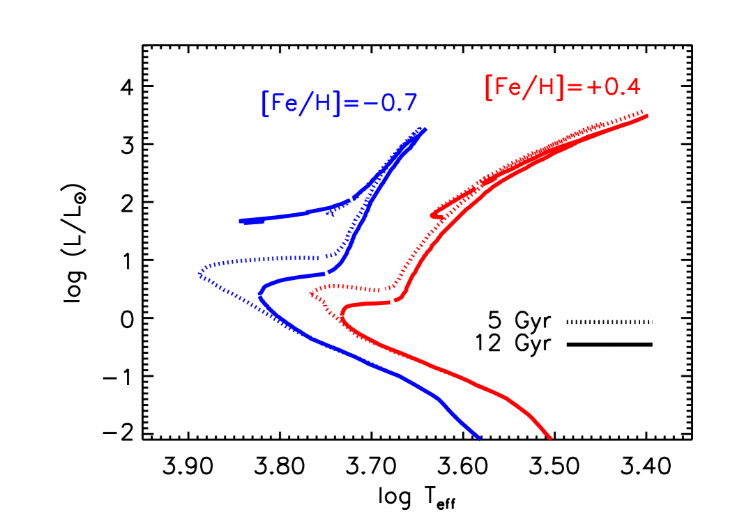


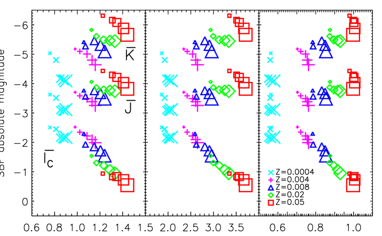
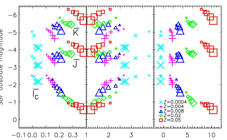

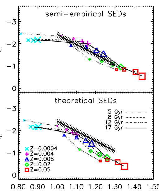
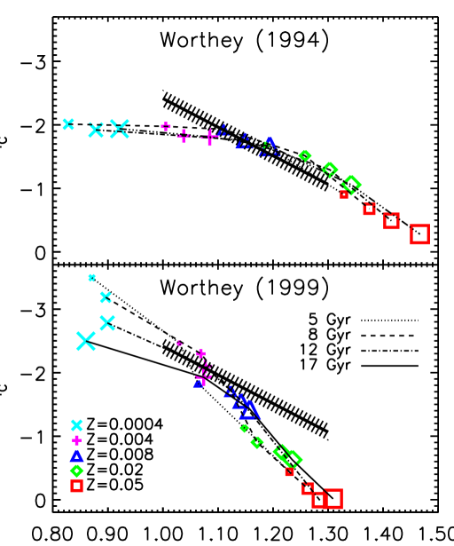
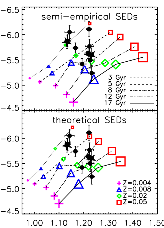
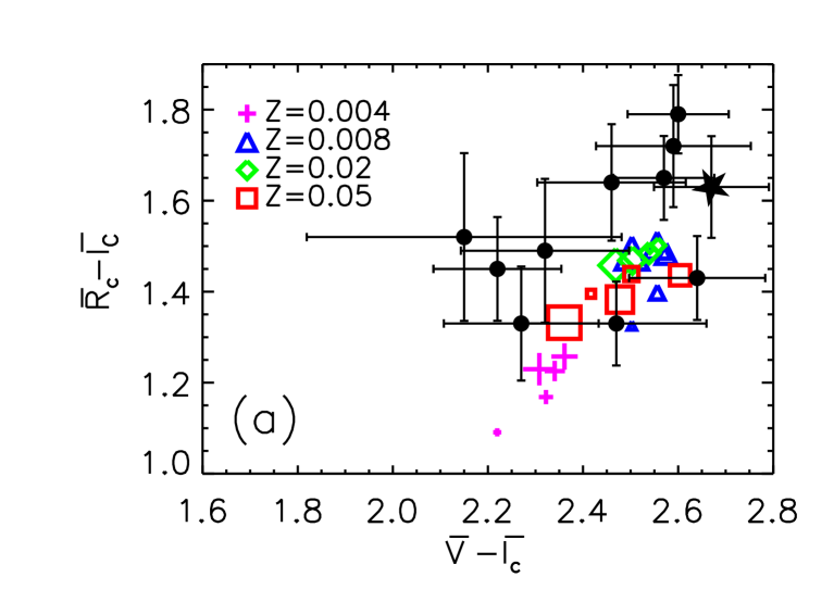
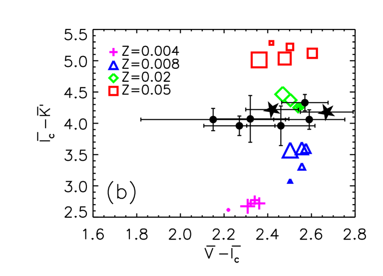
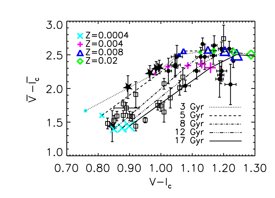
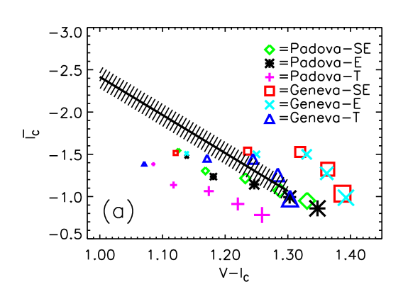
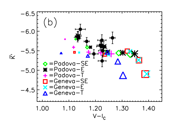
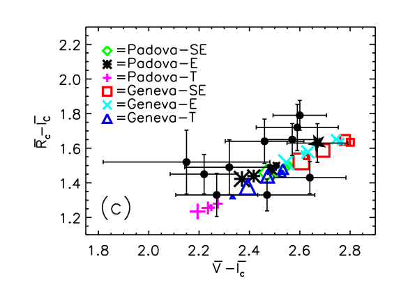
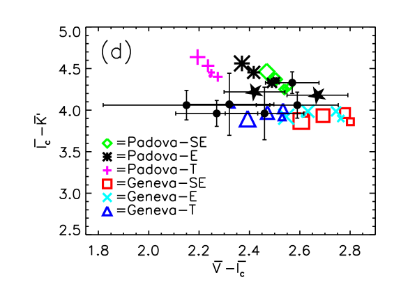
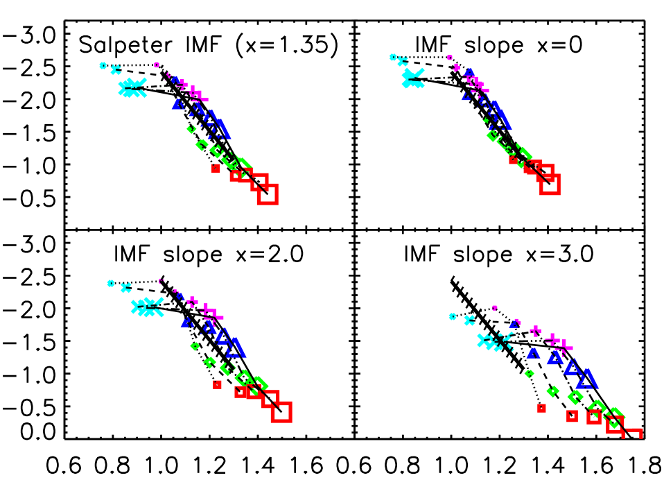
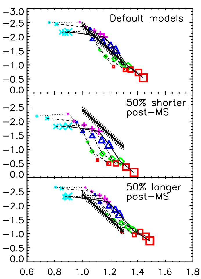
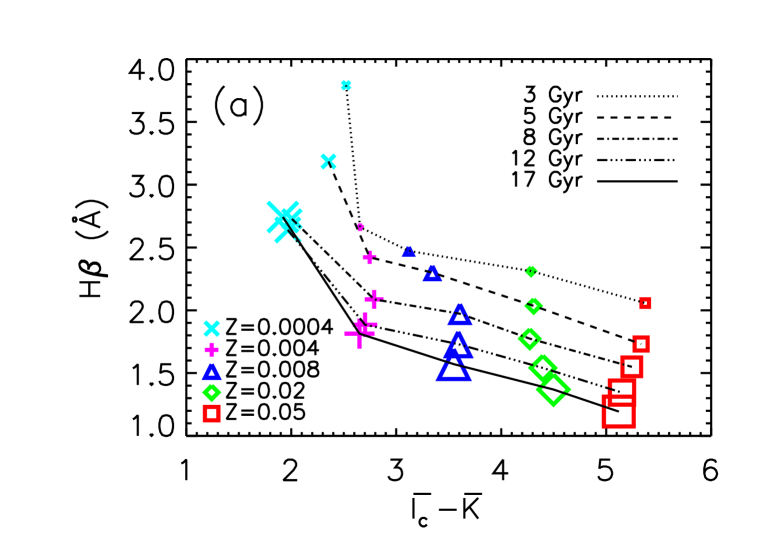
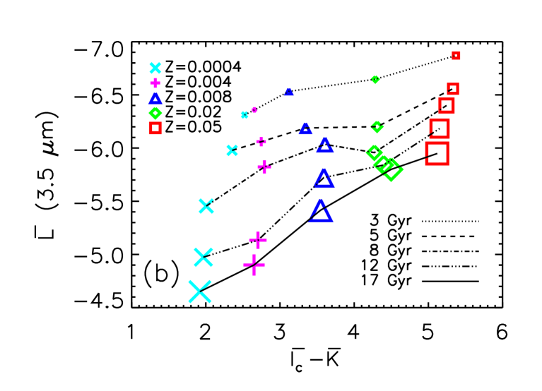
| Inputs | Options | Metallicity RangeaaSolar metallicity is in these models. | Reference |
|---|---|---|---|
| Evolutionary tracks | Geneva | Schaller et al. (1992)bbMore complete lists of references are available in Charlot et al. (1996), Bruzual et al. (1997), and Bruzual & Charlot (2000). | |
| Padova | Bressan et al. (1993)bbMore complete lists of references are available in Charlot et al. (1996), Bruzual et al. (1997), and Bruzual & Charlot (2000). | ||
| Spectral libraries | theoretical | Lejeune et al. (1997, 1998) | |
| semi-empirical | Lejeune et al. (1997, 1998) | ||
| empirical | Pickles (1998) |
Note. — Our standard models use the Padova tracks with the semi-empirical SEDs.
| Gyr | – | – | – | H | Mg2 | Mgb | H | C4668 | ||||||||||||||||||
|---|---|---|---|---|---|---|---|---|---|---|---|---|---|---|---|---|---|---|---|---|---|---|---|---|---|---|
| 0.0001 | ||||||||||||||||||||||||||
| 0.0001 | ||||||||||||||||||||||||||
| 0.0001 | ||||||||||||||||||||||||||
| 0.0001 | ||||||||||||||||||||||||||
| 0.0001 | ||||||||||||||||||||||||||
| 0.0001 | ||||||||||||||||||||||||||
| 0.0001 | ||||||||||||||||||||||||||
| 0.0004 | ||||||||||||||||||||||||||
| 0.0004 | ||||||||||||||||||||||||||
| 0.0004 | ||||||||||||||||||||||||||
| 0.0004 | ||||||||||||||||||||||||||
| 0.0004 | ||||||||||||||||||||||||||
| 0.0004 | ||||||||||||||||||||||||||
| 0.0004 | ||||||||||||||||||||||||||
| 0.0040 | ||||||||||||||||||||||||||
| 0.0040 | ||||||||||||||||||||||||||
| 0.0040 | ||||||||||||||||||||||||||
| 0.0040 | ||||||||||||||||||||||||||
| 0.0040 | ||||||||||||||||||||||||||
| 0.0040 | ||||||||||||||||||||||||||
| 0.0040 | ||||||||||||||||||||||||||
| 0.0080 | ||||||||||||||||||||||||||
| 0.0080 | ||||||||||||||||||||||||||
| 0.0080 | ||||||||||||||||||||||||||
| 0.0080 | ||||||||||||||||||||||||||
| 0.0080 | ||||||||||||||||||||||||||
| 0.0080 | ||||||||||||||||||||||||||
| 0.0080 | ||||||||||||||||||||||||||
| 0.0200 | ||||||||||||||||||||||||||
| 0.0200 | ||||||||||||||||||||||||||
| 0.0200 | ||||||||||||||||||||||||||
| 0.0200 | ||||||||||||||||||||||||||
| 0.0200 | ||||||||||||||||||||||||||
| 0.0200 | ||||||||||||||||||||||||||
| 0.0200 | ||||||||||||||||||||||||||
| 0.0500 | ||||||||||||||||||||||||||
| 0.0500 | ||||||||||||||||||||||||||
| 0.0500 | ||||||||||||||||||||||||||
| 0.0500 | ||||||||||||||||||||||||||
| 0.0500 | ||||||||||||||||||||||||||
| 0.0500 | ||||||||||||||||||||||||||
| 0.0500 |
| as a function of | 7.03 | 4.56 | 0.19 | 6.77 | 4.42 | 0.18 | 1.95 | 1.45 | 0.22 | 2.96 | 1.44 | 0.23 | 2.54 | 2.34 | 0.31 | ||||
| as a function of | 5.59 | 1.36 | 0.10 | 5.38 | 1.32 | 0.10 | 2.14 | 0.52 | 0.17 | 3.12 | 0.53 | 0.19 | 2.90 | 0.83 | 0.24 | ||||
| as a function of | 6.50 | 5.80 | 0.12 | 6.26 | 5.62 | 0.11 | 1.63 | 2.41 | 0.15 | 2.58 | 2.46 | 0.16 | 2.12 | 3.78 | 0.20 | ||||
| as a function of H | 1.05 | 1.41 | 0.33 | 1.07 | 1.37 | 0.32 | 4.29 | 0.31 | 0.26 | 5.26 | 0.30 | 0.27 | 6.34 | 0.53 | 0.38 | ||||
| as a function of Mg2 | 3.10 | 7.13 | 0.11 | 2.96 | 6.91 | 0.11 | 3.14 | 2.58 | 0.19 | 4.13 | 2.58 | 0.20 | 4.45 | 4.13 | 0.26 | ||||
| as a function of Mgb | 3.37 | 0.55 | 0.09 | 3.22 | 0.54 | 0.09 | 3.04 | 0.20 | 0.19 | 4.02 | 0.20 | 0.20 | 4.29 | 0.32 | 0.26 | ||||
| as a function of H | 2.69 | 0.24 | 0.17 | 2.57 | 0.23 | 0.16 | 3.33 | 0.08 | 0.21 | 4.32 | 0.08 | 0.23 | 4.76 | 0.12 | 0.31 | ||||
| as a function of C4668 | 2.37 | 0.19 | 0.15 | 2.25 | 0.18 | 0.15 | 3.35 | 0.08 | 0.16 | 4.34 | 0.08 | 0.17 | 4.81 | 0.12 | 0.21 | ||||
Note. — The fit is for models with and ages of 5, 8, 12, 17 Gyr. The rms scatter about the fitted line is , given in magnitudes.
| 0.004 | ||||||||||
| 0.008 | ||||||||||
| 0.02 | ||||||||||
| 0.05 |
Note. — The term is given by where is the redshift and is the number tabulated above, for different observables (SBF magnitude or galaxy color) as a function model metallicity. The convention for the correction is where is an SBF magnitude or galaxy color. The number in parenthesis is the rms scatter for the linear coefficient averaged over models of different ages (see § 3.4).
| Gyr | – | – | – | H | Mg2 | Mgb | H | C4668 | ||||||||||||||||||
|---|---|---|---|---|---|---|---|---|---|---|---|---|---|---|---|---|---|---|---|---|---|---|---|---|---|---|
| Padova Evolutionary Tracks, Semi-Empirical SEDs (Standard Model) | ||||||||||||||||||||||||||
| 0.02 | ||||||||||||||||||||||||||
| 0.02 | ||||||||||||||||||||||||||
| 0.02 | ||||||||||||||||||||||||||
| 0.02 | ||||||||||||||||||||||||||
| 0.02 | ||||||||||||||||||||||||||
| 0.02 | ||||||||||||||||||||||||||
| 0.02 | ||||||||||||||||||||||||||
| Padova Evolutionary Tracks, Theoretical SEDs (Difference from Standard Model) | ||||||||||||||||||||||||||
| 0.02 | ||||||||||||||||||||||||||
| 0.02 | ||||||||||||||||||||||||||
| 0.02 | ||||||||||||||||||||||||||
| 0.02 | ||||||||||||||||||||||||||
| 0.02 | ||||||||||||||||||||||||||
| 0.02 | ||||||||||||||||||||||||||
| 0.02 | ||||||||||||||||||||||||||
| Padova Evolutionary Tracks, Empirical SEDs (Difference from Standard Model) | ||||||||||||||||||||||||||
| 0.02 | ||||||||||||||||||||||||||
| 0.02 | ||||||||||||||||||||||||||
| 0.02 | ||||||||||||||||||||||||||
| 0.02 | ||||||||||||||||||||||||||
| 0.02 | ||||||||||||||||||||||||||
| 0.02 | ||||||||||||||||||||||||||
| 0.02 | ||||||||||||||||||||||||||
| Geneva Evolutionary Tracks, Semi-Empirical SEDs (Difference from Standard Model) | ||||||||||||||||||||||||||
| 0.02 | ||||||||||||||||||||||||||
| 0.02 | ||||||||||||||||||||||||||
| 0.02 | ||||||||||||||||||||||||||
| 0.02 | ||||||||||||||||||||||||||
| 0.02 | ||||||||||||||||||||||||||
| 0.02 | ||||||||||||||||||||||||||
| 0.02 | ||||||||||||||||||||||||||
| Geneva Evolutionary Tracks, Theoretical SEDs (Difference from Standard Model) | ||||||||||||||||||||||||||
| 0.02 | ||||||||||||||||||||||||||
| 0.02 | ||||||||||||||||||||||||||
| 0.02 | ||||||||||||||||||||||||||
| 0.02 | ||||||||||||||||||||||||||
| 0.02 | ||||||||||||||||||||||||||
| 0.02 | ||||||||||||||||||||||||||
| 0.02 | ||||||||||||||||||||||||||
| Geneva Evolutionary Tracks, Empirical SEDs (Difference from Standard Model) | ||||||||||||||||||||||||||
| 0.02 | ||||||||||||||||||||||||||
| 0.02 | ||||||||||||||||||||||||||
| 0.02 | ||||||||||||||||||||||||||
| 0.02 | ||||||||||||||||||||||||||
| 0.02 | ||||||||||||||||||||||||||
| 0.02 | ||||||||||||||||||||||||||
| 0.02 | ||||||||||||||||||||||||||
Note. — The top set of results gives the model output for our standard solar-metallicity model (Padova evolutionary tracks with semi-empirical SEDs). For all other models, the differences from our standard models are tabulated, e.g., {Geneva model, Pickles SED} – {Padova model, semi-empirical SEDs}.