Rotational Evolution during Type I X-Ray Bursts

Abstract

The rotation rates of six weakly-magnetic neutron stars accreting in low-mass X-ray binaries have most likely been measured by Type I X-ray burst observations with the Rossi X-Ray Timing Explorer Proportional Counter Array. The phenomenology of the nearly coherent oscillations detected during the few seconds of thermonuclear burning is most simply understood as rotational modulation of brightness asymmetries on the neutron star surface. We show that, as suggested by Strohmayer and colleagues, the frequency changes of 1–2 Hz observed during bursts are consistent with angular momentum conservation as the burning shell hydrostatically expands and contracts during the burst. We calculate how vertical heat propagation through the radiative outer layers of the atmosphere and convection affect the coherence of the oscillation. We show that the evolution and coherence of the rotational profile depends strongly on whether the burning layers are composed of pure helium or mixed hydrogen/helium. Our results help explain the absence (presence) of oscillations from hydrogen-burning (helium-rich) bursts that was found by Muno and collaborators.

We also investigate angular momentum transport within the burning layers and address the recoupling of the burning layers with the star. We show that the Kelvin-Helmholtz instability is quenched by the strong stratification, and that mixing between the burning fuel and underlying ashes by the baroclinic instability does not occur. However, the baroclinic instability may have time to operate within the differentially rotating burning layer, potentially bringing it into rigid rotation.

1. Introduction

Type I X-ray bursts have been long understood as thermonuclear flashes on the surfaces of neutron stars accreting at rates of $10^{-11}M_{\odot}\ {\rm yr^{-1}}<\dot{M}<10^{-8}M_{\odot}\ {\rm yr^{-1}}$ in low mass X-ray binaries (LMXBs). The accreted hydrogen and helium accumulates on the surface of the neutron star and periodically ignites and burns. Thermonuclear flash models successfully explain the burst recurrence times (hours to days), energetics ($\sim 10^{39}\,{\rm ergs}$), and durations ($\sim 10$–$100\,{\rm s}$) (Lewin, van Paradijs, & Taam 1993; Bildsten 1998), though many quantitative comparisons to observations are less successful (for example, see Fujimoto et al. 1987; Bildsten 2000).

Table 1Properties of Observed Type I Burst Oscillations

Object	Time	Radius	$\nu_{0}$	$\Delta\nu$	$\tau$	$\Delta\nu/\nu_{0}$	Oscillations	References
	(UT)	Expansion?	(Hz)	(Hz)	(s)	($10^{-3}$)	During Rise?
4U 1636-54	1996 Dec 28 (22:39:22)	Y	580.5	$\approx 1$–$2.5$	$\cdots$	$\approx 2$–$4$	Y	1,2
	1996 Dec 29 (23:26:46)	Y	581.5	$\approx 2$	$\cdots$	$\approx 3$	Y	2,3
	1996 Dec 31 (17:36:52)	Y	581	$\approx 2$	$\cdots$	$\approx 3$	Y	2,3
4U 1702-43	1997 Jul 26 (14:04:19)	?	$329.85\pm 0.1$	2.5	$1.88\pm 0.25$	$7.7\pm 0.3$	Y	4
	1997 Jul 30 (12:11:58)	?	$330.55\pm 0.02$	1.6	$4.02\pm 0.07$	$4.8\pm 0.3$	N	4
4U 1728-34	1996 Feb 16 (10:00:45)	N	$364.23\pm 0.05$	2.4	$3.52\pm 0.28$	$6.6\pm 0.1$	Y	4,5
	1997 Sep 9 (06:42:56)	?	$364.10\pm 0.05$	2.1	$1.84\pm 0.15$	$5.9\pm 0.2$	?	4
KS 1731-26	1996 Jul 14 (04:23:42)	Y	$524.61^{+0.13}_{-0.07}$	$0.96\pm 0.04$	$4.1^{+1.3}_{-0.9}$	1.8	N	6,7
	1999 Feb 27 (17:23:01)	Y	$524.48^{+0.05}_{-0.03}$	$1.06\pm 0.05$	$2.6^{+0.4}_{-0.3}$	2.0	N	7
Galactic Center	1996 May 15 (19:32:10)	Y	589	$\approx 1$	$\cdots$	$\approx 2$	N	8
(MXB 1743-29?)
Aql X-1	1997 Mar 1 (23:27:39)	N	$549.76\pm 0.04$	$2.38^{+0.03}_{-0.07}$	$2.69\pm 0.15$	4.3	N	9,10

Evolutionary scenarios connecting the neutron stars in LMXBs to the millisecond radio pulsars (see Bhattacharya 1995 for a review) predict that neutron stars in LMXBs should be spinning rapidly. This has been confirmed for one system, the $\nu_{s}=401$ Hz accreting pulsar SAX J1808.4-3658 (Wijnands & van der Klis 1998; Chakrabarty & Morgan 1998), in which the neutron star magnetic field ($B\sim 10^{8}$–$10^{9}\ {\rm G}$; Psaltis & Chakrabarty 1999) channels the accretion flow onto the magnetic polar caps, creating an asymmetry which is modulated by rotation. However, most neutron stars in LMXB’s show no evidence for coherent periodicity in the persistent emission, implying that the neutron stars do not possess magnetic fields strong enough to make a permanent asymmetry ($B\ll 10^{10}\,{\rm G}$).

Type I X-ray bursts have provided a new way to determine the spin of these neutron stars. Observations with the Proportional Counter Array (PCA) on the Rossi X-Ray Timing Explorer (RXTE) of neutron stars in six LMXBs have shown coherent oscillations during Type I X-ray bursts, with frequencies $\nu_{0}$ that range from 300 to 600 Hz (see Table 1). The simplest interpretation is that the burning is not spherically symmetric, providing a temporary asymmetry on the neutron star that allows for a direct measurement of rotation. The coherent nature of the periodicities ($Q\gtrsim 300$), large modulation amplitudes and stability of the frequency over at least a year support its interpretation as the neutron star spin (Strohmayer 1999b, and references therein).

It is expected theoretically that the burning should not be spherically symmetric. Joss (1978) and Shara (1982) suggested that ignition of a burst occurs at a local spot on the star, and not simultaneously over the whole surface. This is because it takes hours to days to accumulate the fuel, but only a few seconds for the thermal instability to grow. Simultaneous ignition thus requires synchronization of the thermal state of the accreted envelope to one part in $10^{3}$–$10^{4}$ over the surface. More likely is that ignition is local and a burning front then spreads laterally (Fryxell & Woosley 1982; Nozakura, Ikeuchi, & Fujimoto 1984; Bildsten 1995), burning the rest of the accreted fuel and creating a temporary brightness asymmetry on the neutron star surface (Schoelkopf & Kelley 1991; Bildsten 1995). Consistent with the picture of a spreading burning front, the pulsation amplitude is observed to decrease during the burst rise while the emitting area increases, reaching a constant value during the decay (Strohmayer, Zhang & Swank 1997b; Strohmayer et al. 1998c).

The oscillations during the burst rise are well-explained by the picture of a spreading hotspot. However, several mysteries remain. First, oscillations are often seen in the burst tail, when the whole surface of the star has presumably ignited. The cause of the azimuthal asymmetry at late times is not understood. Secondly, for those objects with $\nu_{0}\approx 550\ {\rm Hz}$ in Table 1, there is evidence that the burst oscillation frequency is twice the spin frequency of the star, including observations of a $\approx 290\ {\rm Hz}$ subharmonic (Miller 1999) and the fact that the kHz QPO separation is approximately half the burst oscillation frequency in these sources (see van der Klis 2000 for a review). What might cause an $m=2$ azimuthal asymmetry is unknown. Third, oscillations are not seen in all sources, or all Type I bursts from the same source.

An initially puzzling feature of the observations was that the oscillation frequency often changes during the burst, increasing by $\Delta\nu\approx 1$–$2$ Hz in the burst tail. Strohmayer et al. (1997a) proposed a simple explanation — that this frequency shift results from angular momentum conservation. The slight hydrostatic radial expansion (contraction) of the burning layers as the temperature increases (decreases) results in spin down (spin up) if angular momentum is conserved. The time for radial heat transport from the burning layers to the photosphere is about one second, which means that the layers are puffed up and spun down by the time the observer sees the burst. As the burning layers cool during the tail of the burst, they contract and spin up. Strohmayer & Markwardt (1999) and Miller (1999, 2000) have modelled the observed frequency evolution. They find that, in the evolving frame of the burning shell, the oscillations are coherent, as expected if they are due to rotation. Calculations show that the change in thickness of the burning layers during a burst is $\Delta z\approx 20\,{\rm m}$ (Hanawa & Fujimoto 1984; Ayasli & Joss 1982; Bildsten 1998). A simple estimate of the spin down of the burning shell due to this change in thickness is then $\Delta\nu\approx\nu_{s}(2\Delta z/R)\approx 1\,{\rm Hz}\,(\nu_{s}/300\,{\rm Hz})(\Delta z/20\,{\rm m})(10\,{\rm km}/R)$ where $R$ is the neutron star radius and $\nu_{s}$ the spin frequency. This roughly agrees with the observed values (Table 1).

In this paper, we make a first attempt at understanding the evolution of the neutron star atmosphere during a Type I X-ray burst on a rotating neutron star. We use hydrostatic models of the neutron star atmosphere to calculate the expansion and resulting spin evolution during a burst. Our aim is to investigate whether the observed frequency changes during bursts are consistent with spin down of the burning shell, thus lending support to the interpretation that the burst oscillation frequency is intimately related to the neutron star spin. This simple picture demands that the hot burning material decouples from the cooler underlying ashes and conserves its angular momentum, completing a few phase wraps with the underlying star during the burst. We thus examine mechanisms that might couple the burning layers to the neutron star, and ask whether it is plausible that the burning layers can remain decoupled for the $\approx 10\,{\rm s}$ duration of the burst.

We stress that we consider only one-dimensional models for these hydrostatic and coupling calculations. We do not consider the complex question of how the burning front spreads around the star during the burst rise, what determines the number of hotspots on the surface, or what causes the asymmetry at late times during the cooling tail of the burst. We leave these questions for future investigations.

We start in §2 by describing the hydrostatic structure of the atmosphere during fuel accumulation and the X-ray burst. In §3, we calculate the expansion of the atmosphere and show that the expected spin down of a decoupled layer is consistent with observed values. We consider heat transport through the atmosphere, and ask how a single coherent frequency is transmitted to the observer. In §4, we discuss hydrodynamic mechanisms that could transport angular momentum within the burning layers or couple the hot burning material to the underlying colder and denser ashes. In §5, we summarize our results and discuss the many remaining puzzles. Finally, we present our conclusions in §6.

2. Thermal Structure and Expansion of the Burning Layers

Most neutron stars in LMXBs accrete hydrogen and helium rich material from their companions at rates $\dot{M}\sim 10^{-11}-10^{-8}M_{\odot}\ {\rm yr^{-1}}$. For accretion rates $\dot{M}\gtrsim 2\times 10^{-10}\,M_{\odot}\ {\rm yr^{-1}}$ (see Bildsten 1998 and references therein), the accumulating hydrogen is thermally stable and burns via the hot CNO cycle of Hoyle & Fowler (1965). The temperature of most of the atmosphere is $\gtrsim 8\times 10^{7}\,{\rm K}$ so that the time for a proton capture onto a ¹⁴N nucleus is less than the time for the subsequent beta-decays. This fixes the energy production rate at the value

$$\epsilon_{H}=5.8\times 10^{13}\left({Z_{\rm CNO}\over 0.01}\right){\rm\ ergs\ g^{-1}\ s^{-1}},$$ (1)

where $Z_{\rm CNO}$ is the mass fraction of CNO nuclei. This energy production rate is independent of temperature or density, and simply set by the beta-decay timescales of ¹⁴O (half-life 71 s) and ¹⁵O (half-life 122 s). Because the hydrogen burns at a constant rate, the time to burn all of it depends only on the metallicity and initial hydrogen abundance. The hydrogen mass fraction $X$ in a given fluid element changes at a rate $dX/dt=-\epsilon_{H}/E_{H}$, where $E_{H}\approx 6.7\,{\rm MeV}/{\rm proton}\approx 6.4\times 10^{18}\,{\rm erg\,g^{-1}}$ is the energy release per gram from burning hydrogen to helium. The time to burn all the hydrogen is then

$$t_{H}\approx 22\ {\rm hours}\ \left({0.01\over Z_{\rm CNO}}\right)\left({X_{0}\over 0.71}\right),$$ (2)

where $X_{0}$ is the initial hydrogen mass fraction.

The X-ray burst is triggered when helium burning becomes unstable at the base of the accumulated layer, at a density $\sim 10^{5}$–$10^{6}\,{\rm g\,cm^{-3}}$ and temperature $\approx 2\times 10^{8}\,{\rm K}$. The composition at the base of the layer depends on how much hydrogen has burned during the accumulation (Fujimoto, Hanawa & Miyaji 1981, hereafter FHM; Bildsten 1998), which is determined by the local accretion rate, $\dot{m}$. The local Eddington accretion rate is $\dot{m}_{\rm Edd}=2m_{p}c/(1+X)R\sigma_{\rm Th}$, where $\sigma_{\rm Th}$ is the Thomson scattering cross-section, $m_{p}$ is the proton mass, $c$ is the speed of light, and $R$ is the stellar radius. In this paper, we use the Eddington accretion rate for solar composition ($X_{0}=0.71$) and $R=10$ km, $\dot{m}_{\rm Edd}\equiv 8.8\times 10^{4}\ {\rm g\ cm^{-2}\ s^{-1}}$, as our basic unit for the local accretion rate (for a 10 km neutron star, this corresponds to a global rate $\dot{M}=1.7\times 10^{-8}\,M_{\odot}\,{\rm yr^{-1}}$). For $\dot{m}\gtrsim 0.03\,\dot{m}_{\rm Edd}$, the helium burning becomes unstable before all the hydrogen is burned and the helium ignites and burns in a hydrogen rich environment. At lower accretion rates $\dot{m}\lesssim 0.03\,\dot{m}_{\rm Edd}$, there is enough time to burn all the hydrogen, and a pure helium layer accumulates which eventually ignites. We now describe simple models of the atmosphere immediately prior to (§2.1) and during (§2.2) the X-ray burst for both of these cases. At lower accretion rates still, $\dot{m}\lesssim 0.01\dot{m}_{\rm Edd}$, the hydrogen burning becomes unstable and triggers a mixed hydrogen/helium burning flash (FHM).

2.1. The Accumulating Atmosphere

Table 2Plane Parallel Ignition Conditions

$\dot{m}/\dot{m}_{\rm Edd}$	$Z_{\rm CNO}$	$T$	$y$	$X$	$Y$	$\rho$	$y/\dot{m}$	$\Delta z$(90%)
		($10^{8}\,{\rm K}$)	($10^{8}\,{\rm g\,cm^{-2}}$)			($10^{6}\,{\rm g\,cm^{-3}}$)	(h)	(m)
Pure He Ignition
0.01	0.005	1.49	5.40	0.0	0.995	2.28	170	4.2
	0.01	1.35	12.9	0.0	0.99	4.14	407	5.1
	0.02	1.22	34.0	0.0	0.98	8.01	1073	6.9
0.015	0.01	1.56	3.67	0.0	0.99	1.75	77	3.8
	0.02	1.41	8.50	0.0	0.98	3.11	179	4.4
0.02	0.01	1.74	1.92	0.0	0.99	1.12	30	3.8
	0.02	1.57	3.62	0.0	0.98	1.74	57	3.5
0.03	0.02	1.83	1.56	0.0	0.98	0.97	16	3.6
Mixed H/He Ignition
0.015	0.005	1.73	2.05	0.01	0.99	1.16	43	4.2
0.02	0.005	1.78	2.18	0.15	0.85	1.04	34	4.5
0.03	0.005	1.86	2.35	0.31	0.69	0.94	25	4.9
	0.01	1.89	1.67	0.14	0.85	0.87	18	4.2
0.1	0.005	2.05	2.70	0.57	0.42	0.84	8.5	5.6
	0.01	2.13	2.04	0.50	0.49	0.71	6.4	5.1
	0.02	2.20	1.51	0.40	0.58	0.62	4.8	4.7
0.3	0.005	2.24	2.62	0.67	0.33	0.76	2.8	5.8
	0.01	2.33	2.14	0.64	0.35	0.66	2.3	5.5
	0.02	2.44	1.70	0.59	0.39	0.57	1.8	5.2

The neutron star atmosphere is in hydrostatic balance as the accreted hydrogen and helium accumulates. The pressure obeys $dP/dz=-\rho g$, where $\rho$ is the density and the gravitational acceleration $g\equiv GM/R^{2}$ is constant in the thin envelope. A useful variable is the column depth $y$ (units g cm^-2), defined by $dy\equiv-\rho dz$, giving $P=gy$. As the matter accumulates, a given fluid element moves to greater and greater column depth. In this paper, we take $g_{14}\equiv g/10^{14}\ {\rm cm\,s^{-2}}=1.9$, appropriate for a $M=1.4\,M_{\odot}$ and $R=10\,{\rm km}$ neutron star. As described above, the hydrogen burning rate is a constant so that the change of $X$ with column depth $y$ is $dX/dy=-\epsilon_{H}/\dot{m}E_{H}$, where we take $E_{H}\equiv 6.4\times 10^{18}\ {\rm erg\ g^{-1}}$ (we have neglected the $\approx 0.5\ {\rm MeV/proton}$ lost as neutrinos in the hot CNO cycle, see Wallace & Woosley 1981). Integrating this equation, we find the hydrogen abundance as a function of depth is

$$X(y)=\cases{X_{0}\left[1-(y/y_{d})\right]&$y>y_{d}$,\cr 0&$y<y_{d}$,\cr}$$ (3)

where $X_{0}$ is the initial hydrogen abundance, and the column depth at which the hydrogen runs out is $y_{d}\equiv X_{0}\dot{m}E_{H}/\epsilon_{H}$, or

$$y_{d}=6.8\times 10^{8}\,{\rm g\,cm^{-2}}\left({\dot{m}\over 0.1\dot{m}_{\rm Edd}}\right)\left({0.01\over Z_{\rm CNO}}\right)\left({X_{0}\over 0.71}\right).$$ (4)

If helium ignites at a column depth $y<y_{d}$, a mixed hydrogen/helium burning flash occurs, otherwise a pure helium layer accumulates which eventually ignites at a column $y>y_{d}$.

The thermal profile of the accumulating layer is described by the heat equation,

$${dT\over dy}={3\kappa F\over 4acT^{3}},$$ (5)

where $\kappa$ is the opacity and $F$ is the outward heat flux. The entropy equation is

$$\epsilon+{dF\over dy}=c_{P}{\partial T\over\partial t}+{c_{P}T\dot{m}\over y}\left({d\ln T\over d\ln y}-n\right)$$ (6)

(Bildsten & Brown 1997), where $n\equiv(d\ln T/d\ln P)_{S}$, $c_{P}$ is the heat capacity at constant pressure, and the terms on the right hand side describe the compression of the accumulating matter. The compressional terms contribute $\approx c_{P}T\approx 5k_{B}T/2\mu m_{p}\approx 20\,T_{8}\ {\rm keV}$ per accreted nucleon, where $\mu$ is the mean molecular weight, and $T_{8}\equiv T/10^{8}\ {\rm K}$. In comparison, the hot CNO cycle hydrogen burning gives $\approx 7X_{0}\ {\rm MeV}$ per accreted nucleon for pure helium ignition, or $\approx 7X_{0}(y_{b}/y_{d})\ {\rm MeV}$ for mixed H/He ignition, where $y_{b}$ is the column depth at the base. There is additional flux from heat released by electron captures and pycnonuclear reactions deep in the crust, giving $\approx 100\ {\rm keV}$ per nucleon (Brown & Bildsten 1998; Brown 2000). For the purposes of this paper, we neglect the compressional terms in the entropy equation, and take

$$\epsilon=-{dF\over dy},$$ (7)

but include a flux at the base ($y=y_{b}$) of $F_{b}=150\ {\rm keV}$ per nucleon as an approximation to the heat from the crust and compressional heating.

We find the temperature profile by integrating equations (5) and (7) from the top of the atmosphere to the base at column depth $y_{b}$. At the top, which we arbitrarily place at $y=5\times 10^{4}\,{\rm g\,cm^{-2}}$, we set the temperature using the analytic radiative zero solution for a constant flux atmosphere with Thomson scattering opacity (the solutions are not sensitive to this upper boundary condition). For $y<y_{d}$ we take $\epsilon=\epsilon_{H}$, and for $y>y_{d}$ we set $\epsilon=0$. The flux at the top $F_{t}$ is set by the energy release from hot CNO burning in the atmosphere and the flux at the base, giving $F_{t}=F_{b}+\epsilon_{H}y_{b}$ or $F_{t}=F_{b}+\epsilon_{H}y_{d}$, whichever is smaller. The opacity $\kappa$ has contributions from electron scattering, free-free absorption and electron conduction, which we calculate as described in Schatz et al. (1999). Since in the hot CNO cycle the seed nuclei are mostly ¹⁴O or ¹⁵O waiting to $\beta$-decay, we take the gas to be a mixture of hydrogen (mass fraction $X$ given by eq.[3]), ¹⁴O and ¹⁵O (mass fraction $Z_{\rm CNO}$) and helium (mass fraction $Y=1-X-Z_{\rm CNO}$). The ratio by number of ¹⁴O to ¹⁵O is given by the ratio of the beta-decay timescales, giving $Z_{14}=0.352Z_{\rm CNO}$ and $Z_{15}=0.648Z_{\rm CNO}$. To obtain a simple analytic estimate of the base temperature, we first integrate equation (7) with $\epsilon_{H}$ a constant to find $F(y)=\epsilon_{H}(y_{b}-y)$, where we ignore compressional heating and the flux from the base. Substituting this into equation (5) and integrating assuming constant opacity, we find $T^{4}(y)=(3\kappa/ac)\epsilon_{H}yy_{b}(1-y/2y_{b})$, giving

$$T_{b}\approx 2.6\times 10^{8}\,{\rm K}\,\left({\kappa\over 0.08\ {\rm cm^{2}\ g^{-1}}}\right)^{1/4}\left({Z_{\rm CNO}\over 0.01}\right)^{1/4}$$

$$\left({y_{b}\over 2\times 10^{8}\,{\rm g\,cm^{-2}}}\right)^{1/2},$$ (8)

where we have inserted a typical value for $\kappa$.

We find the column depth at the base of the accumulated layer just before the thermally unstable helium ignition by comparing the temperature sensitivity of the heating and cooling rates (FHM; Fushiki & Lamb 1987b; Bildsten 1998). The heating rate due to the triple-alpha reaction is

$$\epsilon_{3\alpha}=5.3\times 10^{21}\,{\rm erg\,g^{-1}\,s^{-1}}\ f{\rho_{5}^{2}Y^{3}\over T_{8}^{3}}\exp\left({-44\over T_{8}}\right),$$ (9)

where $f$ is the screening factor (Fushiki & Lamb 1987a). In addition, ¹²C rapidly captures protons once it is made, increasing the energy release from the triple alpha reaction. To account for this, we multiply $\epsilon_{3\alpha}$ by a factor $1+Q_{12}/Q_{3\alpha}=1.9$, where $Q_{3\alpha}=7.274$ MeV, $Q_{12}=Q(^{12}{\rm C}+2p\rightarrow^{14}{\rm O})=6.57$ MeV. An effective local cooling rate is obtained from equations (5) and (7), giving

$$\epsilon_{\rm cool}\approx{acT^{4}\over 3\kappa y^{2}}.$$ (10)

As the matter accumulates, the column depth at the base $y_{b}$ increases until $d\epsilon_{3\alpha}/dT>d\epsilon_{\rm cool}/dT$, at which point a thermal instability occurs (FHM). We find the temperature profile at ignition by choosing $y_{b}$ such that $d\epsilon_{3\alpha}/dT=d\epsilon_{\rm cool}/dT$ at the base. In Figure 1, the hatched region in the temperature-column depth plane indicates where helium ignition occurs for abundances ranging from the initial value ($Y=0.3$) to pure helium ($Y=1.0$).

The conditions at the base of the accumulated column at the time of ignition for a variety of metallicities and accretion rates are shown in Table 2. We have separated our solutions into two groups depending on whether the helium unstably ignites before (mixed H/He ignition) or after (pure He ignition) the hydrogen is completely burned. We give the temperature, density and composition at the base, the time to accumulate the unstable column $y_{b}/\dot{m}$, and the physical distance from the base to the place where $y=y_{b}/10$, $\Delta z(90$%$)$. For mixed H/He (pure He) ignition, $\Delta z(90$%$)\approx 5\ {\rm m}$ ($3.5$–$7\ {\rm m}$).

Figure 1(a) shows the temperature profile of models with mixed H/He ignition. The solid lines are for $Z_{\rm CNO}=0.01$ and (bottom to top) $\dot{m}/\dot{m}_{\rm Edd}=0.03,0.1,0.3$. The dashed lines are for $\dot{m}=0.1\,\dot{m}_{\rm Edd}$ and $Z_{\rm CNO}=0.005$ (bottom curve) or $0.02$ (top curve). Figure 1(b) shows temperature profiles for pure He ignition. The solid lines show $Z_{\rm CNO}=0.01$ and (bottom to top) $\dot{m}/\dot{m}_{\rm Edd}=0.01,0.015,$ and $0.02$. The dashed lines are for $\dot{m}=0.01\,\dot{m}_{\rm Edd}$ and $Z_{\rm CNO}=0.005$ (top curve) or $0.02$ (bottom curve). The black dots show the depth where hydrogen runs out (at a column $y_{d}$, eq. [4]).

For the mixed H/He ignition models, the ignition temperature and density do not depend sensitively on $\dot{m}$. Slight differences arise because at higher accretion rates less helium is made from hydrogen burning, requiring a higher density and temperature for ignition. For pure He ignition, the ignition column and temperature are much more sensitive to accretion rate. After the hydrogen is burned, there is a slight temperature gradient to carry the flux from the base $F_{b}$, but the temperature at ignition is mainly set by the temperature at the base of the hydrogen burning shell (FHM; Wallace, Woosley and Weaver 1982). This temperature is greater at higher accretion rates, leading to a smaller column depth at ignition.

Table 3Models with a Convection Zone

$(y_{b}-y_{c})/y_{b}$	$T_{b}$	$F/F_{\rm Edd}$	$\Delta z_{c}$	$\Delta z$(90%)	$\rho_{b}$	$\beta_{b}$	$\bar{X}$	$\bar{Y}$	$\mu$
	($10^{9}\,{\rm K}$)		(m)	(m)	($10^{5}\ {\rm g\ cm^{-3}}$)
Mixed Ignition
($\dot{m}=0.1\ \dot{m}_{\rm Edd}$; $Z_{\rm CNO}=0.01$; $y_{b}=2.04\times 10^{8}\ {\rm g\,cm^{-2}}$; $\Delta z(90$%$)=5.1\,{\rm m}$)
0.99	1.7	0.89	61.5	40.9	0.83	0.46	0.60	0.39	0.67
0.95	1.7	1.15	48.5	40.7	0.84	0.46	0.60	0.39	0.67
0.8	1.5	0.74	18.3	24.4	1.41	0.67	0.58	0.41	0.68
0.5	1.2	0.31	5.5	15.9	2.30	0.86	0.55	0.44	0.70
Pure He Ignition
($\dot{m}=0.015\ \dot{m}_{\rm Edd}$; $Z_{\rm CNO}=0.01$; $y_{b}=3.67\times 10^{8}\ {\rm g\,cm^{-2}}$; $\Delta z(90$%$)=3.8\,{\rm m}$)
0.99	2.0	1.06	45.6	30.2	2.04	0.42	0.09	0.90	1.16
0.95	1.95	1.21	29.8	25.0	2.45	0.45	0.07	0.92	1.20
0.8	1.6	0.59	8.9	13.1	5.16	0.76	0.01	0.98	1.32
0.5	1.3	0.35	3.1	10.0	7.38	0.90	0.00	0.99	1.35

The effect of increasing metallicity for mixed H/He ignition models is to increase the energy generation rate, and thus the temperature at the base. Together with the increased rate of helium production, this allows He ignition at a lower column depth, as seen in Figure 1(a). For pure He ignition, the effect of increasing metallicity is exactly opposite. The ignition temperature is lowered with increasing metallicity because the hydrogen runs out at a smaller column, giving a smaller temperature at the base of the hydrogen burning shell. Ignition then requires a greater column depth at the base of the almost isothermal pure helium layer, as seen in Figure 1(b).

The $\dot{m}$ at which the transition between pure He and mixed H/He ignitions occurs depends on metallicity. The $\dot{m}=0.02\ \dot{m}_{\rm Edd}$ case in Figure 1 (right panel) just burns the hydrogen before ignition; this is the transition $\dot{m}$ for a metallicity $Z_{\rm CNO}=0.01$. For $Z_{\rm CNO}=0.005$, the transition occurs for $\dot{m}\approx 0.01\ \dot{m}_{\rm Edd}$, and $\dot{m}\gtrsim 0.03\ \dot{m}_{\rm Edd}$ for $Z_{\rm CNO}=0.02$. This is in rough agreement with the $\propto Z_{\rm CNO}^{13/18}$ scaling estimated by Bildsten (1998). The transition accretion rate increases with increasing metallicity because the time to burn all the hydrogen decreases, allowing a pure helium layer to build up even at large accretion rates.

Our results agree well with those of previous authors. The calculations we have presented here are similar to those of Taam (1980) and Hanawa & Fujimoto (1982). Hanawa & Sugimoto (1982) simulated pure He ignition bursts on neutron stars with $g_{14}=0.93$ and $7.1$. Conditions at the base of the hydrogen burning shell that they find agree with our calculations to 10%, and the helium ignition column agrees to within a factor of two. We find similar agreement with the pure He ignition calculations of Wallace, Woosley & Weaver (1982, hereafter W82). However, the density at the base of the hydrogen burning shell that we compute is twice as great as that given in Table 1 of W82, whereas the pressure and temperature agree. We do not know the reason for this discrepancy, but it may be that W82 used a fixed solar composition for the hydrogen burning shell, giving a different value for $\mu_{e}$ at the base. Hanawa & Fujimoto (1984) simulated mixed H/He ignition bursts. Taking into account their gravity, $g_{14}=3.3$, our ignition column and temperature agree with their calculations to 10–30%.

2.2. The Atmosphere During the Burst

Many authors have simulated X-ray bursts for both mixed H/He and pure He ignitions, for reviews see Lewin, van Paradijs, & Taam (1993), and Bildsten (1998). In this section, we make simplified models which allow us to calculate the hydrostatic expansion of the atmosphere during a burst. We do not discuss the lateral spreading of the burning front in this paper. In addition, our models are not appropriate for the radius expansion phase of bursts with super-Eddington luminosities (radius expansion bursts; Lewin, van Paradijs, & Taam 1993). We discuss the effect of radius expansion on the observability of oscillations in §3.5. We start in §2.2.1 by considering the convective stage of a burst. As we discuss later, convection is important because it likely enforces rigid rotation, and may affect the observability of a coherent signal (§3). In §2.2.2 we compute fully-radiative atmospheric models, appropriate for those bursts that do not become convective, or for the later stages of a convective burst, when the convection zone retreats.

2.2.1 Models with Convection

Table 4Fully Radiative Models

$F/F_{\rm Edd}$	$T_{b}$	$\Delta z$(90%)	$\rho_{b}$	$\beta_{b}$	Notes
	($10^{9}\,{\rm K}$)	(m)	($10^{5}\ {\rm g\ cm^{-3}}$)
Mixed Ignition
($\dot{m}=0.1\ \dot{m}_{\rm Edd}$; $Z_{\rm CNO}=0.01$; $y_{b}=2.04\times 10^{8}\ {\rm g\,cm^{-2}}$; $\Delta z(90$%$)=5.1\,{\rm m}$)
1.15	1.49	29.7	1.53	0.68	a
	1.29	25.7	2.13	0.82	b
0.74	1.35	22.3	1.94	0.78	a
	1.17	20.1	2.50	0.88	b
0.31	1.12	15.6	2.67	0.90	a
	0.96	14.5	3.20	0.94	b
Pure He Ignition
($\dot{m}=0.015\ \dot{m}_{\rm Edd}$; $Z_{\rm CNO}=0.01$; $y_{b}=3.67\times 10^{8}\ {\rm g\,cm^{-2}}$; $\Delta z(90$%$)=3.8\,{\rm m}$)
1.21	1.57	16.9	5.44	0.78	a
	1.38	15.4	6.83	0.87	b
0.59	1.34	11.9	7.10	0.88	a
	1.17	11.1	8.35	0.93	b
0.35	1.19	9.9	8.22	0.93	a
	1.04	9.4	9.39	0.96	b

In one-dimensional models, the energy release from the temperature sensitive helium burning reaction makes the early stages of many bursts convective. The convection zone expands outwards, extending over a few scale heights to the radiative outermost layers (Joss 1977). For example, Hanawa & Fujimoto (1984) computed a mixed H/He ignition model, in which the atmosphere was convective for $\approx 1\ {\rm s}$ after ignition, reaching a maximum extent of $\approx 99\%$ of the accumulated mass. Hanawa & Sugimoto (1982) found for pure He ignition that a convection zone rapidly grew to encompass most of the atmosphere, and then shrunk back, disappearing $\approx 1\ {\rm s}$ later when the nuclear fuel was almost exhausted.

The convection in the neutron star atmosphere is very efficient, since the time for sound to cross a scale height ($c_{s}/g\sim 10^{-6}\,{\rm s}$) is much shorter than the local thermal time ($\sim 1$–$10\,{\rm s}$). Thus the atmosphere has a nearly adiabatic profile when convective. For a given temperature $T_{b}$ and column depth $y_{b}$ at the base, the thermal profile of the convective zone just follows the adiabat $T=T_{b}(y/y_{b})^{n}$, where $n\equiv(\partial\ln T/\partial\ln P)_{S}$. We take $y_{b}$ to be the value given by the settling solution at ignition; the convection zone profile is then determined by the single parameter $T_{b}$ when the mean molecular weight, $\mu$, is fixed.

During the burst, the temperature at the base reaches $\gtrsim 10^{9}\,{\rm K}$, high enough that radiation pressure is important (Joss 1977). At these temperatures, the degeneracy is lifted (we find the electron pressure differs from the ideal gas value by less than a few percent) so the total pressure at the base is

$$P_{b}={\rho_{b}k_{B}T_{b}\over\mu m_{p}}+{1\over 3}aT_{b}^{4},$$ (11)

where $\rho_{b}$ is the density at the base. However, the total pressure is also fixed by the weight of the overlying atmosphere, which gives $P_{b}=gy_{b}$. Thus $T_{b}$ cannot exceed the critical value $T_{\rm max}=(3gy_{b}/a)^{1/4}$, or

$$T_{\rm max}=2.2\times 10^{9}\,{\rm K}\,\left({y_{b}\over 3\times 10^{8}\,{\rm g\,cm^{-2}}}\right)^{1/4}\left({g_{14}\over 1.9}\right)^{1/4}.$$ (12)

As $T_{b}$ approaches $T_{\rm max}$, radiation pressure becomes increasingly important, forcing the density to decrease. We show below that this greatly enhances the expansion of the atmosphere.

As clearly argued by Joss (1977), the convection zone cannot extend all the way to the photosphere. A radiative layer is always needed to transport the heat to the photosphere. We assume that most of the burning occurs in the convective layer, in which case the radiative atmosphere carries a constant flux and is described by the heat equation (5) with constant $F$. For the convective zone, we integrate $dT/dy=n(T/y)$ for a given base temperature $T_{b}$ (the super-adiabaticity needed to carry the flux in the convective zone is negligible when the convection is so efficient; see Cox & Giuli 1968). For these simple models, we treat the flux $F$ and base temperature $T_{b}$ as free parameters (in reality, the temperature throughout the convective region determines the nuclear energy generation rate and thus the flux). To compute the thermal profile of the atmosphere, we integrate the convection zone outwards from the base, and the radiative zone inwards from the surface, varying the column depth of the top of the convection zone $y_{c}$ until the temperature matches at the interface.

We compute convective models for a range of fluxes and base temperatures for two of the settling solutions of Figure 1. The first is for the mixed H/He ignition model with $\dot{m}=0.1\,\dot{m}_{\rm Edd}$ and $Z_{\rm CNO}=0.01$. Figure 2(a) shows temperature profiles of convective models with flux $F/F_{\rm Edd}=0.31,0.74,0.89$ and $1.15$, the fraction of the accumulated matter that becomes part of the convective zone, $(y_{b}-y_{c})/y_{b}=0.5,0.8,0.99$ and $0.95$, and base temperature $T_{b}/10^{9}\,{\rm K}=1.2,1.5,1.7$ and $1.7$ respectively. Here we measure flux in units of the Eddington flux (for the accreted solar composition) $F_{\rm Edd}=GM\dot{m}_{\rm Edd}/R$, giving $F_{\rm Edd}\equiv 1.67\times 10^{25}\,{\rm erg\,cm^{-2}\,s^{-1}}$. Figure 2(b) shows convective models corresponding to the pure He ignition settling solution with $\dot{m}=0.015\,\dot{m}_{\rm Edd}$ and $Z_{\rm CNO}=0.01$. We make convective models with flux $F/F_{\rm Edd}=0.35,0.59,1.06$ and $1.21$, the fraction of the accumulated matter that becomes part of the convective zone, $(y_{b}-y_{c})/y_{b}=0.5,0.8,0.99$ and $0.95$, and base temperature $T_{b}/10^{9}\,{\rm K}=1.3,1.6,2.0$ and $1.95$ respectively. Properties of all these models are given in Table 3. In each case, we take the composition profile of the atmosphere to be that immediately prior to ignition, but assume full mixing of matter in the convective zone (we average over the convection zone according to $\bar{X_{i}}\equiv\int dyX_{i}(y)/(y_{b}-y_{c})$ for each species $i$).

We give the thickness of the convection zone $\Delta z_{c}$ in Table 3, as well as the height above the base which contains 90% of the mass, $\Delta z(90\%)$. A simple analytic estimate of the thickness, $\Delta z_{c}$, is obtained as follows. First, the adiabatic index of the gas is

$$n\equiv\left({d\ln T\over d\ln P}\right)_{s}={8-6\beta\over 32-24\beta-3\beta^{2}},$$ (13)

(Clayton 1983), where the ratio of gas pressure to total pressure is

$$\beta=1-0.044\left({T\over 10^{9}\,{\rm K}}\right)^{4}\left({y_{b}\over 3\times 10^{8}\,{\rm g\,cm^{-2}}}\right)^{-1}\left({g_{14}\over 1.9}\right)^{-1}.$$ (14)

For $\beta=1$ ($P=P_{g}$), we obtain the ideal gas value $n=2/5$; for $\beta=0$ ($P=P_{r}$), $n=1/4$. We take $P\propto T^{n}$, and presume $\beta$ is a constant throughout the convective zone, so that $n$ is a constant, given by equation (13). Integrating $dz=-dP/\rho g$, we find the thickness of the convection zone is

$$\Delta z_{c}\approx{H_{b}\over n}\left[1-\left({P_{t}\over P_{b}}\right)^{n}\right],$$ (15)

when it extends to a pressure $P_{t}$. We denote the scale height at the base as $H_{b}\equiv P_{b}/\rho_{b}g=k_{B}T_{b}/\mu m_{p}g\beta$ and assume $\mu$ is constant, giving

$$\Delta z_{c}\approx 11\,{\rm m}\ {T_{9,b}\over\mu\beta}\left({0.4\over n}\right)\left({1.9\over g_{14}}\right)\\ \left[1-\left({P_{t}\over P_{b}}\right)^{n}\right].$$

Using the value of $\beta$ at the base (denoted $\beta_{b}$ in Table 3) to evaluate equation (2.2.1), we find this analytic estimate agrees to better than 5% with the numerical integrations. Equation (2.2.1) shows that radiation pressure strongly affects the radial extent of the convective zone, $\Delta z_{c}\propto 1/\beta$.

We show the density as a function of height above the base for the mixed H/He and pure He ignition models in Figure 3(a) and (b) respectively. The jump in density at the interface between the convective and radiative zones is due to the jump in composition because the convective zone is fully mixed. The black dots mark the height which encloses 90% of the mass as found numerically. This ranges from $\approx 15$–$50\ {\rm m}$ for the mixed H/He models, and $\approx 10$–$30\ {\rm m}$ for the pure He models (Table 3), compared to $\approx 5\ {\rm m}$ before the burst (Table 2). The difference between the mixed H/He and pure He models arises because $\Delta z_{c}$ depends strongly on the mean molecular weight (eq. [2.2.1] gives $\Delta z_{c}\propto 1/\mu$). For a mixture of H and He, $\mu=4/(8X+3Y)$, giving $\mu=4/3$ for pure He, but $\mu=0.6$ for solar composition, almost a factor of two different. The mean molecular weight for each model is given in Table 3.

2.2.2 Fully-Radiative Models

We consider two different kinds of radiative models: a radiative atmosphere carrying constant flux, and a radiative atmosphere with a constant energy production rate $\epsilon$. The first case is relevant when the energy production is concentrated near the base, for example in the initial He burning stages of a burst which does not convect. The second case is relevant when the burning region is more extended. For example, in bursts with mixed H/He ignition, the helium burns rapidly (by purely strong reactions) during the initial stages of the burst, whereas the hydrogen burns more slowly (by the rp-process involving weak reactions; Wallace & Woosley 1981), giving rise to the long tails seen in some X-ray bursts (for a recent example, see Figure 2 of Kong et al. 2000). Because the timescale for H burning by the rp process ($\sim 10$–$100\ {\rm s}$) is long compared to the time for radiative heat transport ($\sim 1$–$10\ {\rm s}$), the atmosphere is radiative during the rp process tail of the burst (Hanawa & Sugimoto 1982).

We give details of our fully-radiative models in Table 4. For the constant $\epsilon$ models, we choose $\epsilon$ to give the required flux at the top, $F=\epsilon y_{b}+F_{b}$. We assume the composition of the atmosphere is the same as immediately prior to ignition. Figure 4 shows the temperature profiles. We compute models with $F/F_{\rm Edd}=0.31,0.74$ and $1.15$ (mixed ignition) and $F/F_{\rm Edd}=0.35,0.59$ and $1.21$ (pure He ignition). Figure 5 shows the density profiles for these models. For the mixed ignition models, $\Delta z($90%$)\approx 15$–$33\ {\rm m}$; for the pure He models, $\Delta z($90%$)\approx 9$–$17\ {\rm m}$. Again, the pure He models are less extended because of the larger $\mu$.

3. Spin Evolution of the Burning Layers

We have shown that the atmosphere expands outwards by $\approx 10$–$50\ {\rm m}$ ($\approx 5$–$25\ {\rm m}$) during a mixed H/He (pure He) burst. In this section, we first calculate how the spin of the burning layers evolves during the burst, assuming they conserve angular momentum as they hydrostatically expand and contract, and that they remain decoupled from the bulk of the neutron star (§3.1–3.3). In §3.4, we point out (in agreement with Miller 2000) that for the observer to see a coherent oscillation requires either a mechanism to enforce rigid rotation of the burning layers (such as convection), or that the burning layers be geometrically thin. In addition, we consider the heat propagation through the radiative layers to the surface, and discuss how this can “wash-out” any coherent pulse emanating from deeper layers. We conclude in §3.5 by discussing what happens during radius expansion bursts.

3.1. Expansion and Spin Down

We assume that the action of hydrodynamic instabilites (Fujimoto 1988, 1993) or a weak poloidal magnetic field will force the accumulating pile of fuel to be rigidly rotating with the spin frequency of the star, $\Omega_{\star}$. The time for angular momentum to diffuse across a scale height $H$ due to molecular viscosity $\nu$ alone is $t_{visc}\approx H^{2}/\nu$. In §5, we show that this time is $t_{visc}\approx 38\,{\rm h}\,(H/5\ {\rm m})^{2}$ for $T_{8}\approx 2$, comparable to the time between bursts. Thus, even microphysical mechanisms might bring the accumulated fuel into corotation.

We further assume that the burning is spherically symmetric, ignoring the complicated, and important, question of how the burning spreads over the stellar surface, and the fact that some asymmetry is needed to give an observable oscillation. Thus we assume the angular velocity is constant on spherical shells, and depends on radius only. This remains true as the atmosphere expands, since a rigidly rotating spherical shell stays rigidly rotating as it expands outwards (because the fractional change in the distance from the rotation axis is the same for all latitudes). Conservation of angular momentum demands that $r^{2}\Omega(r)$ remains constant as a fluid element expands outwards, giving the spin frequency as a function of column depth during the burst

$$\Omega(y)=\Omega_{\star}\left({R+z_{1}(y)\over R+z_{2}(y)}\right)^{2},$$ (16)

where $z_{1}(y)$ ($z_{2}(y)$) is the height of column $y$ above the base before (during) the burst. We take the base at $y_{b}$ to be at fixed radius $R$, even though the old ashes below heat up and expand a little. We ignore the general relativistic corrections to the frequency shift, which Strohmayer (1999a) estimates are a $\approx$10%–20% effect.

Equation (16) shows that the spin frequency depends on depth in the radiative layers. The picture is different in a convective zone. We expect the convective motions will rapidly bring the convection zone into rigid rotation, since the convective turnover time is very short ($\sim 10^{-3}\,{\rm s}$). Thus, if there is no angular momentum transport between the convective zone and neighboring layers, the spin frequency of the convective zone is

$$\Omega_{c}=\Omega_{\star}\left({I_{1}\over I_{c}}\right),$$ (17)

where $I_{1}$ is the total moment of inertia of the material between $y_{c}$ and $y_{b}$ before the ignition, and $I_{c}$ is the moment of inertia of the convection zone. We calculate the moment of inertia as follows. A spherical shell at radius $r$, mass $dm=4\pi r^{2}\rho\,dr$ has a moment of inertia $dI=(8\pi/3)\rho(r)r^{4}\,dr$, where the $8\pi/3$ comes from integrating over angles. Since $\rho dr\equiv-dy$, this is $dI=-(8\pi/3)r^{4}dy$. Thus the moment of inertia is

$$I(y)={8\pi R^{4}\over 3}\int_{y_{b}}^{y}dy\left(1+{z(y)\over R}\right)^{4},$$ (18)

where $z(y)$ is the height above the base, given by integrating $dz/dy=-1/\rho$. We take $P=gy$ during this integration, neglecting the small variation of $g$ with depth, which has an ${\cal O}(H/R)^{2}$ effect on the moment of inertia.

We derive a simple analytic estimate of the moment of inertia of the convective zone, by assuming $\beta=P_{g}/P$ is constant, so that $z(P)$ is given by an equation similar to equation (15). Inserting this into equation (18), writing $(1+z/R)^{4}\approx 1+4z/R$ and integrating, we find

$$I_{c}={2\over 3}\Delta M_{c}R^{2}\left[1+{4H_{b}\over nR}\left(1-{1\over n+1}{1-x^{n+1}\over 1-x}\right)\right],$$ (19)

where $x\equiv y_{c}/y_{b}$, and $\Delta M_{c}\equiv 4\pi R^{2}(y_{b}-y_{c})$ is the mass of the convection zone. The moment of inertia has two pieces. The zeroth order piece, $2\Delta M_{c}R^{2}/3$ is the moment of inertia of mass $\Delta M_{c}$ concentrated at radius $R$. The second term is the ${\cal O}(H/R)$ correction to this because the envelope is extended. Equation (19) reproduces the numerical results to a few percent.

The lower panels of Figure 2 show $\Delta\Omega/\Omega(y)\equiv(\Omega_{\star}-\Omega(y))/\Omega_{\star}$ as a function of column depth for the different convective models in Table 3. We define $\Delta\Omega/\Omega$ so that a positive value means that the layers have spun down. Figure 4 shows $\Delta\Omega/\Omega(y)$ for the fully radiative models of Table 4. The values of $\Delta\Omega/\Omega$ that we find are similar to the observed frequency shifts during bursts (Table 1). As we described above, in radiative zones the spin down depends on height, whereas convective zones are rigidly rotating. In the convective models, this gives rise to jumps in $\Delta\Omega/\Omega$ at the boundaries between the convection zone and both the underlying ashes and the overlying radiative layer. For both convective and fully-radiative models, the $\Delta\Omega/\Omega(y)$ is smaller by roughly a factor of two for pure He ignition as opposed to mixed H/He ignition. This is because the pure He models expand outwards less, as we discussed in §2.2.

3.2. Shrinking of the Convection Zone

As we described in §2.2.1, the atmosphere does not remain convective for the whole duration of the burst. Eventually, the convection zone shrinks back. What is the profile of $\Delta\Omega/\Omega$ left by the retreating convection zone? Imagine that the convection zone retreats by an amount $dy_{c}$ (so the top of the convection zone moves from column $y_{c}$ to $y_{c}+dy_{c}$). The material which decouples from the convection zone takes away an amount of angular momentum given by $dJ_{c}=-8\pi(R+\Delta z_{c})^{4}\Omega_{c}dy_{c}/3$, where $\Omega_{c}$ is the spin frequency of the convection zone, and $\Delta z_{c}$ is the height of the top of the convection zone above the base. The loss of angular momentum from the convection zone must be compensated by a change in its spin or moment of inertia $dJ_{c}=d(I_{c}\Omega_{c})=I_{c}d\Omega_{c}+\Omega_{c}dI_{c}$. Dividing by $dy_{c}$, and changing variables to $x\equiv y_{c}/y_{b}$, we obtain the differential equation

$${d\Omega_{c}\over dx}=-{\Omega_{c}\over I_{c}}\left[{8\pi R^{4}y_{b}\over 3}\left(1+{\Delta z_{c}\over R}\right)^{4}-{dI_{c}\over dx}\right].$$ (20)

We integrate this equation from the starting values of $\Omega_{c}$ and $x$, towards $x\rightarrow 1$ as the convection zone vanishes. There is one difficulty, however, which is that $\Delta z_{c}$ and $I_{c}$ are functions of not only $x$ but also the scale height at the base $H_{b}$. If we assume the composition $\mu$ does not change, then $H_{b}$ only depends on $T_{b}$. We model $T_{b}(x)$ as follows,

$$T_{b}(x)=T_{0}+\Delta T\left({1-x\over 1-x_{i}}\right),$$ (21)

where $T_{0}$ is the final temperature after the convection vanishes ($x\rightarrow 1$), $T_{0}+\Delta T$ is the initial temperature at the base of the convection zone, and $x_{i}$ is the initial value of $x$. In reality, $x$ is determined by the instantaneous values of $F$ and $T_{b}$, so if we knew $F(T_{b})$ we could map this onto $T_{b}(x)$. Instead, we specify $T_{b}(x)$ then as a check that our choice is reasonable, we can compute $F(T_{b})$.

Figure 6 shows the results for the model with $\dot{m}=0.1\dot{m}_{\rm Edd}$, $Z_{\rm CNO}=0.01$ (mixed H/He ignition), with initial extent of the convective zone $(y_{b}-y_{c})/y_{b}=0.8$, and base temperature $T_{b}/10^{9}\,{\rm K}=1.5$. As the convection zone retreats, we assume the base temperature falls to $T_{b}/10^{9}\,{\rm K}=1.0$. We show $\Delta\Omega/\Omega$ profiles for the initial model (80% of mass convective), an intermediate case (50%) and when the convective zone has almost vanished (5%). These models have $T_{b}/10^{9}\,{\rm K}=1.5,1.31,$ and $1.03$ and $F/F_{\rm Edd}=0.74,0.49,$ and $0.21$ respectively. The jumps in $\Delta\Omega/\Omega$ at the top and base of the convection zone persist as it shrinks. In addition, the matter that becomes radiative spins up as the physical thickness of the underlying convection zone decreases. This gives rise to an inversion in $\Delta\Omega/\Omega$, as shown in Figure 6. One might worry that such an inverted profile would be unstable to axisymmetric perturbations. However, all the profiles in Figure 6 have increasing specific angular momentum with radius. In addition, the Brunt-Väisälä frequency is so large, $N^{2}\gg\Omega^{2}$ (§4.1), that we expect the Solberg-Hoiland criterion for stability (see e.g. Endal & Sofia 1978) will always be satisfied.

3.3. Spin Up in the Cooling Tail

As the atmosphere cools in the tail of a burst, its thickness decreases, and it spins back up. We compute simple models of the cooling atmosphere by assuming it carries a constant flux and has a fixed uniform composition. In Figure 7 we show the thickness $\Delta z($90%$)$ as a function of the flux $F/F_{\rm Edd}$. The solid curve is for the $\dot{m}=0.1\ \dot{m}_{\rm Edd}$, $Z_{\rm CNO}=0.01$ mixed H/He ignition model, for which we assume a composition of ⁷³Kr, since the rp process makes elements beyond the iron group (Schatz et al. 1998 and references therein; Koike et al. 1999). The dashed lines are for pure He ignitions, with $Z_{\rm CNO}=0.01$, $\dot{m}=0.01\ \dot{m}_{\rm Edd}$ (upper curve) and $\dot{m}=0.015\ \dot{m}_{\rm Edd}$ (lower curve), and for a composition ⁵⁶Ni. In each case, we show $\Delta z(90$%$)$ just before ignition by a horizontal solid line.

Figure 7 shows that in the limit $F/F_{\rm Edd}\rightarrow 0$, the thickness of the ashes is about half the pre-burst thickness for mixed H/He ignition, but similar to the pre-burst thickness for pure He ignition. This is because electrons (which provide most of the pressure support) are consumed in hydrogen burning, but not during helium burning. In the tail of a burst, when, for example $F/F_{\rm Edd}\approx 0.1$, the thickness of the atmosphere is $\approx 1\ {\rm m}$ different from the pre-burst thickness in both cases. Thus if the burning layers remain decoupled as they cool, we expect the spin frequency in the tail to be different from the stellar spin by a part in $\approx 10\ {\rm km}/1\ {\rm m}\approx 10^{4}$. We discuss the implications of this result in §5.3.

3.4. Heat Transport and Coherence of the Oscillation

We now turn to the vertical transport of heat, and its effect on the coherence and amplitude of the burst oscillations. Figures 2 and 4 show that in a radiative zone the magnitude of the spin down depends on depth. However, a single coherent frequency is observed during bursts. This implies that either convection or some other mechanism (see §4) is enforcing rigid rotation in the burning region, or, as pointed out by Miller (2000), the burning layers must be geometrically thin. Since the fractional change in spin across a height $\Delta z$ in a radiative zone is $\approx 2\Delta z/R$, an observed coherence $Q$ demands a burning layer thickness $\lesssim R/2Q$. Strohmayer & Markwardt (1999) found $Q\approx 4000$ for bursts from 4U 1728-34 and 4U 1702-43 when the observed frequency evolution was accounted for, while Muno et al. (2000) found $Q\approx 5000$ for burst oscillations from KS 1731-26. These results imply a burning region thickness $\lesssim 100\ {\rm cm}$. This is perhaps more likely for pure He bursts, because of the temperature sensitivity of He burning reactions.

Also important is heat transport across the differentially-rotating atmosphere. The time for radial heat transport from the burning layers to the photosphere can be estimated from the entropy equation, $c_{P}\partial T/\partial t=\partial F/\partial y$, together with equation (5) for the flux $F$, which gives a timescale $t_{\rm therm}=3\kappa c_{P}y^{2}/4acT^{3}$. In our numerical calculations, we calculate the heat capacity at constant pressure $c_{P}$ exactly. We make an analytic estimate for a mixture of ideal gas and radiation using $c_{P}=(5k_{B}/2\mu m_{p})f(\beta)$ where $f(\beta)=(32-24\beta-3\beta^{2})/5\beta^{2}$ (Clayton 1983), giving

$$t_{\rm therm}=0.6\,{\rm s}{f(\beta)\over\mu}\left({\kappa\over 0.08\,{\rm cm^{2}\,g^{-1}}}\right){y_{8}^{2}\over T_{9}^{3}}.$$ (22)

The factor $f(\beta)$ is unity for $\beta=1$ ($P=P_{g}$) and grows increasingly larger as $\beta$ approaches zero ($P=P_{r}$), for example $f(0.85)=2.6$ whereas $f(0.4)=27$ (this is because the internal energy of a photon gas at constant pressure is independent of temperature). Thus at a fixed pressure, the thermal time first decreases with increasing temperature (since $t_{\rm therm}\propto 1/T^{3}$) but starts increasing again once radiation pressure becomes important.

Equation (22) shows that the thermal time ($\sim 1\ {\rm s}$) is much longer than the time for hydrostatic readjustment ($\sim 10^{-6}\ {\rm s}$), explaining why spin down is not seen in the beginning of a burst. By the time the heat released by nuclear burning reaches the observer, the layers have expanded and spun down.

The burning layers revolve around the underlying star in a time $\Delta\nu^{-1}\equiv 2\pi/\Delta\Omega\approx 1\ {\rm s}$, comparable to the thermal time. The ratio of the shearing time to the thermal time is important. If the heat diffuses quickly, $t_{\rm therm}\Delta\nu\ll 1$, the atmosphere simply transmits the burning pattern from below, much like passing a flashlight behind a piece of paper. If, on the other hand, heat diffuses slowly, the oscillations will be smeared out. In the limit $t_{\rm therm}\Delta\nu\gg 1$, the atmosphere is heated uniformly by the quickly revolving burning layers.

Figure 8 shows $t_{\rm therm}$ (solid line) and $\Delta\nu^{-1}$ (hatched region for $\nu_{s}=300$–$600\ {\rm Hz}$) as a function of depth for the convective models of Table 3. For mixed H/He and pure He ignitions, the wrap around time $\Delta\nu^{-1}$ increases for decreasing base temperature and physical thickness. The thermal time, however, decreases with decreasing temperature at a given depth because radiation pressure (eq. [22]) is less important. Figure 8 shows that the mixed H/He ignition bursts have $t_{\rm therm}\Delta\nu\approx 1$, whereas the pure He ignition bursts have $t_{\rm therm}\Delta\nu\lesssim 1$. This is because both the spin down and thermal time are less for the pure helium bursts ($\Delta z_{c}\propto 1/\mu$ and $t_{\rm therm}\propto 1/\mu$). As we discuss further in §5.2, Figure 8 may explain the lack of burst oscillations seen in bursts with the characteristics of mixed H/He ignition. For these mixed H/He ignition bursts, $t_{\rm therm}\Delta\nu\approx 1$ and any oscillations in the flux from deeper regions can get washed out.

3.5. Radius Expansion Bursts

Many of the bursts which have shown oscillations are radius expansion bursts (Table 1), in which super-Eddington luminosities result in expansion of the photosphere to radii $\sim 20$–$100\ {\rm km}$ (for a review see Lewin, van Paradijs, & Taam 1993). Burst oscillations have not been observed during the peak of radius expansion bursts, but are sometimes seen during the burst rise, and often during the tail of the burst, once the photosphere has fallen back to the stellar radius $R$ (for an example, see Figure 2 of Strohmayer et al. 1998c which shows a radius expansion burst from 4U 1636-54).

We did not model radius expansion in §3. However, several of our models have super-Eddington fluxes, and thus are appropriate for the early stages of these bursts. Because the opacity deep in the atmosphere is smaller than at the photosphere, the hydrostatic structure we calculate breaks down only in the very upper layers near the photosphere. Our radiative models are also appropriate for the cooling tail of these bursts, when the photosphere has fallen back to the stellar surface.

Whatever the cause of the asymmetry on the neutron star surface, the fact that oscillations are not seen during the peak of radius expansion bursts is as we would expect, given the discussion of §3.4. The long thermal time across the extended envelope during radius expansion (Paczynski & Anderson 1986), as well as the fact that the horizontal and vertical lengthscales are similar, will hide any asymmetry and wash out the oscillation.

4. Angular Momentum Transport and Recoupling

We have shown that if different layers of the atmosphere conserve their angular momentum, expansion during the burst results in differential rotation within the burning layers. Thus as we noted in §3.4, the fact that a single coherent frequency is observed implies that either the burning layers are geometrically thin, or that they must rotate rigidly. While convection may enforce rigid rotation in the early stages of a burst, we do not expect the atmosphere to be convective in the cooling tail (see §2.2). In this section, we investigate mechanisms which might transport angular momentum between the differentially-rotating burning layers. In addition, we investigate whether the burning layers can remain decoupled from the underlying cold ashes for the $\approx 10\ {\rm s}$ duration of the burst and the implied several phase wraps.

4.1. Kelvin-Helmholtz Instability

Shear layers are notoriously unstable to hydrodynamic instabilities, in particular the Kelvin-Helmholtz instability (Chandrasekhar 1961). The shear may be stabilized by buoyancy, however, if the work that must be done against gravity to mix up the fluid is greater than the kinetic energy in the shear. The importance of buoyancy is measured by the Richardson number, ${\rm Ri}=N^{2}/(dU/dz)^{2}$ (for example, see Fujimoto 1988), where $N$ is the Brunt-Väisälä frequency, a measure of the buoyancy. The Kelvin-Helmholtz instability occurs when ${\rm Ri}<1/4$ (Chandrasekhar 1961; Fujimoto 1988).

There are two sources of buoyancy in the atmosphere, thermal buoyancy and buoyancy due to the composition gradient. We write the Brunt-Väisälä frequency $N$ as

$$N^{2}={g\over H}\left[{\chi_{T}\over\chi_{\rho}}\left(n-{d\ln T\over d\ln y}\right)+{\chi_{\mu_{e}}\over\chi_{\rho}}{d\ln\mu_{e}\over dz}+{\chi_{\mu_{i}}\over\chi_{\rho}}{d\ln\mu_{i}\over dz}\right]$$ (23)

(Bildsten & Cumming 1998), where $\chi_{Q}\equiv\partial\ln P/\partial\ln Q$ with the other independent thermodynamic variables held constant. The first term of equation (23) is the thermal buoyancy. For an ideal gas atmosphere carrying a constant heat flux in which the opacity is Thomson electron scattering opacity, this is $N_{th}^{2}=3\mu m_{p}g^{2}/20k_{B}T$ (Bildsten 1998), giving

$${N_{th}\over 2\pi}\approx{3\times 10^{4}\ {\rm Hz}\over T_{9}^{1/2}}\left({\mu\over 0.6}\right)^{1/2}\left({g_{14}\over 2}\right).$$ (24)

We estimate the composition gradient terms as $N^{2}_{\mu}\approx g\Delta\ln\mu/H$, giving

$${N_{\mu}\over 2\pi}\approx 7\times 10^{4}\ {\rm Hz}\left(\Delta\ln\mu\right)^{1/2}\left({10\ {\rm m}\over H}\right)^{1/2},$$ (25)

where we have taken the density scale height $H$ as the lengthscale over which the mean molecular weight changes by $\Delta\ln\mu\sim{\cal O}(1)$.

We show the Brunt-Väisälä frequency during the burst for two fully-radiative models in the top panel of Figure 9. We show the mixed H/He ignition model with $F=0.83\ F_{\rm Edd}$, and the pure He ignition model with $F=0.59\ F_{\rm Edd}$ (see Table 4). We show the total buoyancy by a solid line, the thermal buoyancy as a dotted line and the composition piece as a dashed line. For the pure He ignition model, there is a peak in the buoyancy at the place where the hydrogen runs out ($y\approx y_{d}$), at this depth the composition piece of the buoyancy dominates the thermal piece. Our models do not include the composition jump at the base between the burning layers and the ashes. The point marked by a cross at the base of each model shows an estimate of the buoyancy at the base, where we estimate the composition piece of the buoyancy using equation (25) and take the ashes to have $\mu=2.1$ (for a single species, $\mu=A/1+Z$).

The Richardson number ${\rm Ri}=N^{2}/(dU/dz)^{2}$ is plotted in the lower panel of Figure 9 for $\nu_{s}=300$–$600\ {\rm Hz}$. Since $\Delta\Omega\approx(2z/R)\Omega$, we estimate $dU/dz=Rd\Delta\Omega/dz\approx 2\Omega$, giving

$${\rm Ri}\approx 7000\ \left({\nu_{s}\over 300\ {\rm Hz}}\right)^{-2}\left({N\over 5\times 10^{4}\ {\rm Hz}}\right)^{2},$$ (26)

which agrees well with Figure 9. As suggested by Bildsten (1998), the strong buoyancy in the atmosphere gives ${\rm Ri}\gg 1$. Thus we do not expect the Kelvin-Helmholtz instability to operate either within the burning layers or between the burning layer and the underlying ashes.

4.2. Ekman Pumping

We now investigate how fast viscosity acts to smooth out differential rotation. The molecular viscosity in the atmosphere is determined by ion-ion collisions, giving

$$\nu\approx 88\ {\rm cm^{2}\,s^{-1}}\,\left({T_{9}^{5/2}\over\rho_{5}}\right)\left({A^{1/2}\over Z^{4}}\right)\left({8\over\log\Lambda}\right)$$ (27)

(Spitzer 1962), where $T_{9}\equiv T/10^{9}\,{\rm K}$, $\rho_{5}\equiv\rho/10^{5}\,{\rm g\,cm^{-3}}$ and $\log\Lambda$ is the Coulomb logarithm. Thus the time for molecular viscosity to transport angular momentum over a scale height by diffusion is

$$t_{\nu}\approx 3.2\ {\rm h}\ \left({H\over 10\ {\rm m}}\right)^{2}\left({\nu\over 88\ {\rm cm^{2}\,s^{-1}}}\right)^{-1},$$ (28)

much longer than a rotation period. In this case, it is possible to exchange angular momentum on a faster timescale than $t_{\nu}$ by the process of Ekman pumping. This mechanism involves a secondary circulation in which fluid elements are exchanged between the bulk of the fluid and the thin viscous boundary layer. Ekman pumping is well-studied in fluid dynamics (Benton & Clark 1974), and Livio & Truran (1987) suggested that it may operate in accreting white dwarfs. For a non-stratified fluid, the Ekman spin up or spin down time is $t_{E}\approx(t_{\nu}/\Omega)^{1/2}$ or

$$t_{E}\approx 2.5\ {\rm s}\ \left({t_{\nu}\over 3.2\ {\rm h}}\right)^{1/2}\left({\nu_{s}\over 300\ {\rm Hz}}\right)^{1/2}$$ (29)

(Greenspan & Howard 1963; Benton & Clark 1974). The thickness of the viscous boundary layer is $\approx(\nu/\Omega)^{1/2}\approx 0.2\ {\rm cm}\ (\nu/88\ {\rm cm^{2}\,s^{-1}})^{1/2}(\nu_{s}/300\ {\rm Hz})^{-1/2}$.

Spin up in a stratified fluid is different since the buoyancy may inhibit vertical motion of fluid elements, limiting the extent of the secondary circulation. Spin up in a cylinder of radius $a$ with $g$ parallel to $\Omega$ was first studied by Holton (1965; see Benton & Clark 1974 for a review). In this case, the secondary circulation is confined to a layer of vertical thickness $\approx a(\Omega/N)$ (Walin 1969). Sakurai, Clark & Clark (1971) found a similar result for a spherical stratified fluid, for which Ekman spin up occurs in a thin layer of radial extent $\approx R(\Omega/N)$. The neutron star atmosphere during a burst has $H<R(\Omega/N)\approx 60\ {\rm m}$. Thus, if the spherical result is applicable to a thin layer on the surface of a sphere, we would not expect the buoyancy to inhibit Ekman pumping. In addition, we have $t_{\rm therm}\approx t_{E}$, so non-adiabatic effects may be important, reducing the effect of the thermal buoyancy (Sakurai et al. 1971). Detailed calculations are needed to find whether Ekman pumping operates during the burst.

4.3. Baroclinic Instability

The baroclinic instability is a hydrodynamic instability in which the fluid motions are close to horizontal, so it occurs even when the Richardson number is large. It has been well-studied in geophysics (Pedlosky 1987) and in astrophysics because of its possible role in angular momentum transport in stellar interiors (Knobloch & Spruit 1982; Tassoul & Tassoul 1982; Spruit & Knobloch 1984) and accreting compact objects (Fujimoto 1988, 1993). We start by showing that in the presence of a vertical shear, the surfaces of constant pressure and density are inclined with respect to each other. This represents a store of gravitational energy which the baroclinic instability can tap. We then present the results of a stability analysis of a plane-parallel model, for which we find that the strong buoyancy limits the baroclinic instability to short vertical wavelengths ($\lesssim 200\ {\rm cm}$).

4.3.1 The Nature of the Baroclinic Instability

We first study the misalignment of the constant density and pressure surfaces that arises in the presence of vertical shear on a rotating star. This result is well-known on the Earth, where differential heating between the equator and pole gives rise to the “thermal wind” (Pedlosky 1987). To investigate recoupling of the ashes and burning layers, we adopt a simple “two layer” model, in which we include only the buoyancy associated with the interface between the ashes and the burning layers. Thus, we take the upper (lower) layer to have constant density $\rho_{+}$ ($\rho_{-}$). Both layers are in hydrostatic balance in the vertical direction. As elsewhere in this paper, we assume the burning front has spread over the whole surface.

We work in the rotating frame, in which the lower fluid is stationary. We assume the upper layer is rigidly rotating with angular velocity $-\Delta\Omega$ (so that $\Delta\Omega$ is positive for a spun down shell). Since it is moving, the upper fluid feels a Coriolis force in the transverse direction. In a time $\approx\Omega^{-1}\approx 10^{-3}\ {\rm s}$, a transverse pressure gradient will be established which balances the Coriolis force (geostrophic balance). However, in the lower fluid there is no transverse pressure gradient (it feels no Coriolis force). Since the pressure must be continuous across the boundary, it cannot be horizontal, but must slope.

Figure 10(a) illustrates this. We show a small section of the two layers at latitude $\theta$ ($\theta$ is the angle from the pole) in the $(r,\theta)$ plane. Because the star is rotating, the equilibrium isobars are not spherical, but nearly (the stellar radius is larger at the equator than the pole by $\approx R^{2}\Omega^{2}/g\approx 100\ {\rm m}$ for typical parameters). We adopt coordinates $z$ and $y$ perpendicular and parallel to surfaces of constant pressure (dotted line). The vertical component of the rotation vector is $\Omega\cos\theta$, and the upper fluid is moving out of the page with velocity $U=R\Delta\Omega\sin\theta$.

Now consider the pressure changes as we move from point A to point B on the boundary. First we move through the lower fluid along the dashed line, horizontally a distance $dy$, then vertically upwards a distance $dz$. The pressure change along this path is $dP_{-}=-\rho_{-}g\,dz$. Second, we move through the upper fluid along the dashed line. This time, there is a pressure change while moving horizontally also, giving $dP_{+}=-\rho_{+}g\,dz-\rho_{+}2\Omega U\cos\theta\,dy$. Demanding $dP_{-}=dP_{+}$, gives the slope

$${dz\over dy}={2\Omega^{2}R\over g}{\Delta\Omega\over\Omega}{\rho_{+}\over\Delta\rho}\cos\theta\sin\theta,$$ (30)

where $\Delta\rho=\rho_{-}-\rho_{+}>0$. If we take the equilibrium equipotentials to be spherical ($dy\approx Rd\theta$) and integrate, we find the change in height of the boundary is $z_{b}(\theta)=-\bar{z}_{b}\cos 2\theta+\,{\rm const.}$, where $\bar{z}_{b}=(\Omega^{2}R^{2}/2g)(\Delta\Omega/\Omega)(\rho_{+}/\Delta\rho)$ or

$$\bar{z}_{b}=35\ {\rm cm}\ \left({\nu_{s}\over 300\ {\rm Hz}}\right)^{2}\left({\Delta\Omega/\Omega\over 4\times 10^{-3}}\right)\left({\rho_{+}\over\Delta\rho}\right),$$ (31)

where we have taken $g_{14}=2$ and $R=10\ {\rm km}$.

The sloping interface represents a store of gravitational potential energy. Assuming constant density, the displaced mass per unit area is $\rho z_{b}(\theta)$, and the gravitational energy per unit area required to displace the interface is $\rho gz_{b}(\theta)^{2}/2$. Integrating over a spherical surface, we find the gravitational energy stored in the interface is $\Delta E_{g}=(16/45)(4\pi R^{2}\rho_{+}g\bar{z}_{b}^{2}/2)(\Delta\rho/\rho_{+})$, or

$$\Delta E_{g}=6\times 10^{34}\ {\rm erg}\ \left({\Delta\rho\over\rho_{+}}\right)\left({\bar{z}_{b}\over 35\ {\rm cm}}\right)^{2}$$

$$\left({\rho_{+}\over 10^{5}\ {\rm g\ cm^{-3}}}\right)\left({g_{14}\over 2}\right).$$ (32)

The amount of displaced mass is $\approx 4\pi R^{2}\rho\bar{z}_{b}\approx 4\times 10^{19}\ {\rm g}$, so $E_{g}$ is only a few keV per nucleon, much less than the energy produced by nuclear burning. Thus establishing the sloping interface poses no energetic obstacle. For comparison, the energy in the shear is $\approx\rho H_{b}U^{2}/2$ per unit area, giving $E_{U}\approx(8\pi R^{2}/3)\rho H_{b}(R\Delta\Omega)^{2}/2$ or

$$E_{U}\approx 3\times 10^{34}\ {\rm erg}\ \left({\rho\over 10^{5}\ {\rm g\ cm^{-3}}}\right)\left({H_{b}\over 10\ {\rm m}}\right)$$

$$\left({\nu_{s}\over 300\ {\rm Hz}}\right)^{2}\left({\Delta\Omega/\Omega\over 4\times 10^{-3}}\right)^{2},$$ (33)

when integrated over the surface.

The baroclinic instability acts to release the gravitational potential energy stored in the misaligned pressure and density surfaces. Consider the fluid displacements shown in Figure 10(b). If the fluid element is displaced to point A, it is heavier than its new surroundings and is pushed back by the buoyancy of the interface. However, if it is moved to point B, it falls in the gravitational field, releasing energy. Any displacement within the so-called “wedge of instability” (Pedlosky 1987) is convectively unstable in this way.

4.3.2 Results of Stability Analysis

We have carried out a linear stability analysis of a plane parallel two-layer model. We do not present our detailed calculations, rather we summarize our results and use simple physical arguments to understand them. We start by considering motions about a latitude $\theta=\theta_{0}$, and adopting a local cartesian coordinate system $(x,y,z)$ where the transverse coordinate $x$ ($y$) is in the $\phi$ ($\theta$) direction. We include the effect of sphericity using the “beta-plane approximation” of geophysics (Pedlosky 1987), i.e. we write

$$2\Omega\sin\theta\approx 2\Omega\sin\theta_{0}+(\theta-\theta_{0})\cos\theta_{0},$$ (34)

where we assume $(\theta-\theta_{0})=y/R\ll 1$. We consider a channel centered on $\theta_{0}=\pi/4$ and of width $\pi R/4$, stretching from the pole to the equator. We write the fluid displacement as ($\xi_{x}$,$\xi_{y}$,$\xi_{z}$), and look for solutions $\propto\exp({\sigma t+ik_{x}x+ik_{y}y})$ where $k_{x}=2\pi/\lambda_{x}$ and $k_{y}=2\pi/\lambda_{y}$ are the transverse wavenumbers, and $\sigma$ is the growth rate. Pedlosky (1987) performs a similar analysis, although restricted to the case $\Delta\rho/\rho\ll 1$.

We find that small wavelengths are stable because the fluid displacements lie outside the wedge of instability. To see this, assume that the perturbations are in geostrophic balance, in which case the continuity equation gives $\xi_{z}/\lambda_{z}\approx{\rm Ro}\,\xi_{\perp}/\lambda_{\perp}$, where ${\rm Ro}\approx U/2\Omega\lambda_{\perp}\approx R\Delta\Omega/2\Omega\lambda_{\perp}$ is the Rossby number of the perturbation, and the transverse wavelength $\lambda_{\perp}=2\pi/k_{\perp}$, with $k_{\perp}^{2}=k_{x}^{2}+k_{y}^{2}$. Then the angle of fluid displacement is $\xi_{z}/\xi_{y}\approx\xi_{z}/\xi_{\perp}\approx R\Delta\Omega H/\lambda_{\perp}^{2}\Omega$, where the vertical wavelength is set by the vertical extent of the burning layers $\lambda_{z}\approx H$. For instability, the angle of fluid displacement should be less than the slope of the interface (eq. [30]), requiring $\lambda_{\perp}^{2}\gtrsim(gH_{b}/\Omega^{2})(\Delta\rho/\rho_{+})$, or

$$\lambda_{\perp}>\lambda_{BC}=7.5\times 10^{5}\ {\rm cm}\ \left({H_{b}\over 10\ {\rm m}}\right)^{1/2}\left({g_{14}\over 2}\right)^{1/2}$$

$$\left({\Delta\rho\over\rho_{+}}\right)^{1/2}\left({\nu_{s}\over 300\ {\rm Hz}}\right)^{-1},$$ (35)

where we insert the correct prefactor. Thus the nearly horizontal unstable displacements require transverse wavelengths of order the stellar radius or greater.

However, very large transverse wavelength perturbations can be stabilized because the vertical component of $\Omega$ changes significantly across a wavelength. The changing vorticity provides a restoring force in the $\theta$ direction (Pedlosky 1987). This is the same force which supports Rossby waves (Pedlosky 1987; Brekhovskikh & Goncharov 1994; Dutton 1995). We find that the convective instability overcomes the Rossby wave restoring force when the shear velocity is greater than the Rossby wave speed, $U>U_{\rm Ro}\approx 2\Omega\lambda_{\perp}^{2}/R$ (see also Pedlosky 1987). Thus we require $\lambda_{\perp}\lesssim R(\Delta\Omega/\Omega)^{1/2}$, or

$$\lambda_{\perp}<\lambda_{\rm Ro}=3.3\times 10^{5}\ {\rm cm}\ \left({\Delta\Omega/\Omega\over 4\times 10^{-3}}\right)^{1/2}\left({R\over 10\,{\rm km}}\right)$$ (36)

for instability, where we insert the correct prefactor.

Transverse wavelengths which satisfy equation (4.3.2) do not satisfy equation (36). Thus in the context of our plane-parallel model, we conclude that, when $H=10\ {\rm m}$, large scale mixing between the burning layers and ashes by the baroclinic instability does not occur. Instability can occur when $\lambda_{\rm BC}<\lambda_{\rm Ro}$, or $\Delta\rho/\rho_{+}\lesssim(4\Omega^{2}R/g)(\Delta\Omega/\Omega)(R/H)$. Since $\Delta\Omega/\Omega\approx 2H/R$, this is

$${\Delta\rho\over\rho_{+}}\lesssim 0.15\ \left(\nu_{s}\over 300\ {\rm Hz}\right)^{2}\left({g_{14}\over 2}\right),$$ (37)

so mixing may occur as the burning layers cool and the density contrast with the ashes decreases. The growth rate of an unstable mode is $\propto k_{x}$, so that writing $k_{x}\approx m/R$ (so that $e^{ikx}\sim e^{im\phi}$), we estimate the fastest growing modes will have $m\approx 20\ (\lambda_{\perp}/3\times 10^{5}\ {\rm cm}$). Several authors have studied two layer models on a sphere (Hollingsworth 1975; Hollingsworth, Simmons & Hoskins 1976; Simmons & Hoskins 1976, 1977; Moura & Stone 1976; Warn 1976), but for parameters of interest for the Earth, namely $\Delta\rho/\rho\ll 1$ and $\Delta\Omega/\Omega\approx 0.01$. They find good agreement with growth rates calculated with beta-plane models. However, further calculations are needed to extend our analysis to the spherical case, and determine the spherical eigenfunctions and growth rates.

4.3.3 Short Wavelength Modes

So far we have considered only vertical wavelengths $\lambda_{z}\approx H$, because of the simple vertical structure of the two layer model. However, if we allow perturbations with $\lambda_{z}<H$, we expect to find instability for small enough vertical wavelengths. This is because for small vertical wavelengths, the fluid displacement is able to lie within the wedge of instability (Figure 10) while still having a transverse wavelength which is unaffected by Rossy wave restoring forces (eq. [36]).

We make a simple estimate of the vertical wavelength at which instability occurs by repeating the arguments leading to equation (4.3.2), but this time allowing $\lambda_{z}<H_{b}$. In this case, $\lambda_{BC}$ is given by equation (4.3.2) with $H_{b}$ replaced by $\lambda_{z}$. For instability, we require $\lambda_{\rm BC}<\lambda_{\rm Ro}$ (eq. [36]) giving

$$\lambda_{z}\lesssim 200\ {\rm cm}\ \left({\Delta\Omega/\Omega\over 4\times 10^{-3}}\right)\left({\nu_{s}\over 300\ {\rm Hz}}\right)\left({\rho_{+}\over\Delta\rho}\right),$$ (38)

where we take $g_{14}=2$ and $R=10\ {\rm km}$. We expect modes with vertical wavelengths small enough to satisfy equation (38) to be unstable.

Fujimoto (1988, 1993) used the short wavelength baroclinic modes to define a turbulent viscosity $\nu_{\rm turb}\approx\lambda_{z}^{2}/t_{\rm grow}$ where the growth time of the instability is $t_{\rm grow}\approx\nu_{s}^{-1}{\rm Ri^{1/2}}$, or

$$t_{\rm grow}\approx 0.25\ {\rm s}\ \left({\nu_{s}\over 300\ {\rm Hz}}\right)^{-1}\left({{\rm Ri}\over 7000}\right)^{1/2}$$ (39)

(Pedlosky 1987; Fujimoto 1988). The time to transport angular momentum across a scale height is $t_{\nu}\approx H^{2}/\nu_{\rm turb}\approx t_{\rm grow}(H/\lambda_{z})^{2}$, or

$$t_{\nu}\approx 6\ {\rm s}\ \left({t_{\rm grow}\over 0.25\ {\rm s}}\right)\left({H\over 10\ {\rm m}}\right)^{2}\left({\lambda_{z}\over 200\ {\rm cm}}\right)^{-2}$$ (40)

Thus turbulent transport of angular momentum driven by the short wavelength baroclinic modes could be important during a burst. In particular, these could act to force the burning shell to rigidly rotate.

4.4. Magnetic Field Winding

The majority of neutron stars in LMXBs show no evidence for coherent pulsations in their persistent emission. This implies that these neutron stars are weakly magnetic ($B\ll 10^{9}\ {\rm G}$) so the accretion flow is likely not disrupted before it reaches the neutron star surface. We now ask what effect would a weak magnetic field have on the shearing atmosphere during a burst? The Ohmic diffusion time across a scale height is $t=4\pi\sigma H^{2}/c^{2}$, or

$$t_{\rm diffuse}\approx{10^{7}\,{\rm s}\over Z}\ \left({H\over 10\ {\rm m}}\right)^{2}\left({T\over 10^{9}\ {\rm K}}\right)^{3/2}\left({8\over\log\Lambda}\right)$$ (41)

(Brown & Bildsten 1998) where we estimate the conductivity as

$$\sigma\approx{2(2k_{B}T)^{3/2}\over\pi^{3/2}m_{e}^{1/2}Ze^{2}\log\Lambda}$$ (42)

(Spitzer 1962), $Z$ is the mean ionic charge and $\log\Lambda$ is the Coulomb logarithm. Since $t_{\rm diffuse}\gg 10\ {\rm s}$, the MHD limit applies during the burst and the shearing atmosphere will bend the magnetic field lines. An initially poloidal magnetic field would prevent the shearing if the energy density in the field is greater than the shear energy, $B^{2}/8\pi>\rho(R\Delta\Omega)^{2}/2$, or

$$B>10^{10}\ {\rm G}\ \rho_{5}^{1/2}\left({R\over 10\ {\rm km}}\right)\left({\Delta\Omega/\Omega\over 4\times 10^{-3}}\right).$$ (43)

This is a similar limit to those from lack of persistent pulsations and from spectral modelling (Psaltis & Lamb 1998). The observed shearing for ten seconds most likely rules out fields this strong.

What can we say about a weaker, initially poloidal field like that often discussed for the the progenitors of millisecond pulsars, $B\sim 10^{8}-10^{9}\ {\rm G}$? Fields this weak can also have a significant effect when in the ideal MHD limit. In this case, the horizontal shearing and dragging of the field lines generates a strong toroidal field. Spruit (1999) recently considered the interaction of magnetic fields and differential rotation in stellar interiors. He considered an initially poloidal field $(B_{z},B_{\theta},0)$, and showed that $B_{\phi}$ grows with time according to $B_{\phi}=NB_{z}$ where $N$ is the number of windings, $N=R\sin\theta\int|\mbox{\boldmath$\displaystyle\nabla$}\Omega|dt$. We have $\mbox{\boldmath$\displaystyle\nabla$}\Omega\approx\Delta\Omega/H$, giving $N\approx(R\Delta\Omega/H)t\approx 2\Omega t$. Thus we find $B_{\phi}\approx B_{z}$ after only a few revolutions of the star, much less than the wrap around time of the shear ($\approx 1\ {\rm s}$). The toroidal field grows so quickly because the field is sheared on a vertical scale $H\ll R$. Another way to see this is to consider a vertical tube of fluid in the shearing region (with height $H$ and cross-section area $A_{i}$) that encloses a magnetic flux $\Phi=B_{z}A_{i}$. After one differential wrapping time (roughly one second), this fluid element will be stretched into a very thin tube of length $2\pi R$ and so will have shrunk in cross-sectional area to $A_{f}=A_{i}H/2\pi R$. If flux-freezing holds, then after one second, $B_{\phi}\approx B_{z}A_{i}/A_{f}\approx B_{z}2\pi R/H\approx 10^{4}B_{z}$.

This simple argument says that an initial field of $\approx 10^{6}\ {\rm G}$ can become dynamically important during the burst. However, further theoretical investigations are needed to see if the implied wrapping of the field is possible without instabilities setting in. If correct, this result implies that the bursters with frequency drift have magnetic fields much weaker than the $B\sim 10^{8}$–$10^{9}\ {\rm G}$ fields usually assumed.

4.5. Summary of Coupling Mechanisms

We have investigated a number of different mechanisms that could enforce rigid rotation within the burning layers, or act to couple the burning layers to the underlying ashes. We find that the strong buoyancy of the atmosphere prohibits the Kelvin-Helmholtz instability and mixing between the ashes and the burning layers by the baroclinic instability. Short vertical wavelength baroclinic modes within the burning region may be unstable and vigorous enough to force the burning layers to rigidly rotate. The timescale for viscosity to act via an Ekman pumping mechanism may be a few seconds or less (eq. [29]), but the effect of buoyancy, in particular from the composition gradients, is not clear. Finally, our initial estimates suggest that winding of a weak magnetic field by the differential rotation is important during the burst.

In summary, we have not found a robust hydrodynamical mechanism that recouples the burning layers to the star during the $\approx 10\ {\rm s}$ burst duration. It thus seems plausible that the burning layers remain decoupled throughout the burst. Short wavelength baroclinic instabilities may operate within the burning layers, although more work is needed to see whether they cause the burning shell to rigidly rotate.

5. Discussion

We now summarize the hydrostatic expansion of the atmosphere during a Type I X-ray burst, and the implied spin evolution of the decoupled burning layers. We find the expected spin changes are of the same order as the observed frequency drifts, thus supporting the picture proposed by Strohmayer et al. (1997a). We then use our results to address two observational issues: (i) why oscillations are not seen in all bursts, and (ii) the observed long term stability of the oscillation frequency.

5.1. Temporal Evolution of the Burning Shell

The atmospheric evolution during the burst is shown schematically in Figure 11 for (a) mixed H/He ignition and (b) pure He ignition. As revealed by one-dimensional simulations, the rapid energy release from helium burning reactions makes the initial stages of most bursts convective. Later in the burst, the convection zone retreats, leaving a purely radiative atmosphere. Figure 12 shows the thickness of the atmosphere which contains 90% of the mass, $\Delta z(90$%$)$, as a function of the flux for constant flux radiative atmospheres (solid and dotted lines) and for the convective models of Table 3 (solid and open squares). For the radiative models, the upper curve is for a composition profile the same as at ignition, while the lower curve is for a composition of ⁷³Kr (⁵⁶Ni) for the mixed H/He (pure He) case, chosen to represent the products of burning. Initially, the evolution of the thickness of the layer is along or above the upper curve as it ignites and heats up, depending on the extent of the convection zone. As nuclear burning proceeds, the mean molecular weight increases, and the thickness decreases, eventually moving back along the lower curve as the atmosphere cools. Just before ignition (upper curve, $F\ll F_{\rm Edd}$), the thickness of the accumulated layer is $\approx 5\ {\rm m}$. During the burst, the atmosphere expands hydrostatically by $\Delta z\approx 10$–$40\ {\rm m}$ ($\approx 5$–$20\ {\rm m}$) for mixed H/He (pure He) ignition. For a given flux, the convective models have a greater thickness than fully-radiative models because the temperature profile is steeper in the convection zone, giving a larger base temperature (compare Tables 3 and 4). As we showed in §2.2, radiation pressure plays an important role when $F\approx F_{\rm Edd}$, acting to lower the density and increase the hydrostatic expansion.

We showed in §3 that in a radiative atmosphere, the magnitude of the spin down depends on depth. Thus to observe a single, coherent frequency requires either the atmosphere to be rigidly rotating, or the burning region to be vertically thin (Miller 2000), so the differential rotation across it is small. Convection may enforce rigid rotation; however, one-dimensional calculations of bursts show that convection persists only for the first $\lesssim 1\ {\rm s}$ of the burst when the energy production is dominated by temperature sensitive and rapid helium burning reactions. In §4, we found that short wavelength baroclinic instabilities may act to enforce rigid rotation within the burning layers. Theoretical studies of detailed burst models and further investigations of angular momentum transport mechanisms are needed to determine whether a coherent pulse is possible once convection has ceased.

To compare the predicted spin down with observed values, we assume that some mechanism operates to enforce rigid rotation within the burning layers, but that the burning layers remain decoupled from the underlying ashes, as suggested by the results of §4. Figure 13 shows the spin evolution of the atmosphere assuming that the whole atmosphere rigidly rotates. For both convective and fully-radiative models, we ignore any differential rotation, and assume $I\Omega$ is constant, where $I$ is the moment of inertia of the atmosphere (eq. [18]). As in Figure 12, the evolution during the burst is shown by the arrows, first the atmosphere spins down as flux increases, then spins back up as burning proceeds, increasing the mean molecular weight, and as the atmosphere cools. To compare with observations, we also indicate the observed frequency shifts (Table 1). For those bursts in which the oscillation frequency was seen only in the tail (Table 1), we plot $\Delta\Omega/\Omega$ as a lower limit, since some cooling will have occurred before the oscillation is first seen.

Figure 13 shows that the change in spin frequency for pure He ignition models is less than that for mixed H/He ignition, because of the smaller hydrostatic expansion. For the largest frequency shifts observed, $\Delta\Omega/\Omega\approx 8\times 10^{-3}$, pure He ignition models require a base temperature very close to the limiting value from radiation pressure (eq. [12]) and $F>F_{\rm Edd}$, so that the density at the base is decreased, enhancing the expansion. It is much easier to get $\Delta\Omega/\Omega$ values this large with mixed H/He ignition, although as we describe below, all bursts with oscillations so far have the characteristics of pure He bursts.

In §3, we found that the time for heat to diffuse from the burning layers to the photosphere is $\approx 1\ {\rm s}$. This delay explains why the spin down of the atmosphere is not observed at the beginning of a burst; the expansion occurs before the signal is seen. We have also shown that the vertical propagation of heat through the atmosphere can affect the oscillation amplitude. A requirement for a large amplitude oscillation is that the time to transport heat from the burning layers (or the top of the convection zone) to the photosphere must be small compared to the shearing time across the atmosphere $\approx\Delta\nu^{-1}$. If so, the shearing atmosphere transmits the burning pattern from below, much like passing a flashlight under a piece of paper. If not, the oscillation will be smeared out, the atmosphere being heated uniformly by the quickly revolving burning layers.

Our results show that there are important differences in spin evolution depending on whether the helium ignites in a pure helium or mixed H/He environment. Because of the greater mean molecular weight of pure helium as opposed to a solar composition, the expansion of the atmosphere in pure He bursts is roughly half that of mixed H/He bursts, giving a smaller $\Delta\Omega/\Omega$ (Figure 13). Also, the ratio of thermal time to shearing time is smaller for a pure helium atmosphere, and the energy production more localized because of the temperature sensitivity of He burning reactions, increasing the likelihood of observing coherent oscillations for pure He bursts.

5.2. Why Do Some Bursts Show Oscillations, But Not All?

A puzzle is that oscillations are not seen in bursts from all sources, or in all bursts from a particular source. So far, there has been only one study of the relation between burst oscillations and properties of the bursts. Muno et al. (2000) studied nine X-ray bursts from KS 1731-26 which occurred during observations with ${\it RXTE}$ at various times between 1996 July and 1999 February. They found that bursts which show coherent oscillations are of short duration ($\approx 10\ {\rm s}$), show radius expansion, and have high peak flux. These characteristics are typical of helium rich bursts. Bursts with longer durations typical of H burning showed no oscillations. More studies are needed to see if this is a general result for other sources. Certainly all reported burst oscillations that we can find appear to be in bursts of short duration typical of pure He ignition. As far as we are aware, oscillations have not been detected in bursts of long duration ($>50\ {\rm s}$) typical of H burning.

Why should only pure-He ignition bursts show oscillations? The differences we find between pure He and mixed H/He bursts may provide an explanation. As we described in §3.4 (see Figure 8), we find that the thermal time is less and the shearing time is greater for pure helium bursts, making it more likely that a large amplitude oscillation from deep regions may propagate outwards.

5.3. Long Term Stability of the Oscillation Frequency

The frequency evolution reported for six bursts is well fit by the model $\nu(t)=\nu_{0}-\Delta\nu e^{-t/\tau}$, where $\nu_{0}$ is the frequency in the burst tail, $\Delta\nu$ the amount by which the oscillation frequency changes and $\tau$ the decay time. The parameters of these fits are given in Table 1. The observed decay times $\tau\approx 2$–$7\ {\rm s}$ are similar to the expected cooling time of the burning layers (eq. [22]). However, we found in §4 that there are mechanisms that might couple the burning layers to the star on a similar timescale. Can we distinguish between these two possibilities observationally?

Figure 12 shows that if the burning layers remain decoupled, the frequency observed in the burst tail will not be that of the neutron star spin. Because of the greater mean molecular weight of the ashes, the thickness of the cooling atmosphere in the tail is different to the initial thickness by $\approx 1\ {\rm m}$. This change in thickness depends on how complete the burning was, so that variations in the energetics and burning in the burst would translate into a scatter of $\approx 1$ part in $10^{4}$ in the final frequency. If the oscillation frequency could be shown to be more stable than this from one burst to the next, it would imply that the ashes and burning layers must recouple during the burst decay. This is complicated due to Doppler shifts from the orbital motion of the neutron star, which change the observed frequency at a level $\approx 2\times 10^{-3}(v_{\rm orb}/600\ {\rm km\ s^{-1}}$) across the orbit. Strohmayer et al. (1998b) showed that two bursts from 4U 1636-54 showed a frequency difference consistent with orbital Doppler shifts, while two bursts from 4U 1728-34 separated by more than one year showed the same asymptotic frequency to $\approx 1$ part in $10^{4}$ (see Table 1). If the orbital parameters are known and the orbital Doppler shift accounted for, more measurements such as these would indicate whether recoupling occurs in the burst tail.

6. Conclusions

We have shown that the hydrostatic expansion, spin down, and later spin up during contraction of the neutron star atmosphere naturally explains the magnitude and sign of the observed changes in the nearly coherent oscillations observed in Type I X-ray bursts. Our results support the simple picture proposed by Strohmayer et al. (1997a) to explain the frequency evolution seen in Type I bursts, and thus the identification of the burst oscillation frequency with the neutron star spin.

The amplitude of the oscillation is set not only by the lateral extent of the asymmetry on the neutron star surface, but also by the vertical propagation of heat through the shearing atmosphere. In addition, we find that the spin behavior differs depending on whether the burst results from pure He ignition or He ignition in a H-rich environment. The spin down is smaller by roughly a factor of two for pure He ignition as opposed to mixed H/He ignition, because the pure He models expand outwards less due to the larger mean molecular weight. In addition, the time for heat propagation through the atmosphere is smaller for pure He models.

This might explain why oscillations have not been detected during bursts of long duration ($\gtrsim 30\ {\rm s}$) typical of H burning (for example, the bursts from GS 1826-24 shown in Figures 2 and 5 of Kong et al. 2000). In particular, the recent study of Muno et al. (2000) of bursts from KS 1731-26 found oscillations only during those bursts with short durations $\approx 10\ {\rm s}$, typical of pure He ignition. However, the largest values of $\Delta\Omega/\Omega$ that are observed (for 4U 1702-43 and 4U 1728-34) require base temperatures very close to the limiting value from radiation pressure for pure He bursts, and this may prove to be a problem. More observational studies of the phenomenology of burst oscillations and their relation to burst properties and source properties, in particular accretion rate, are needed. With further theoretical work, these studies could give us important clues as to how the nature of nuclear burning during bursts depends on accretion rate, and help to resolve the disagreement with one-dimensional models first found with EXOSAT (Bildsten 2000 and references therein).

We have not found a robust hydrodynamical mechanism that recouples the burning layers to the underlying star in the $\approx 10\ {\rm s}$ burst duration. However, the coherence of the observed burst oscillations suggests that little differential rotation occurs within the burning layer itself. As we note in §4, this might be accomplished through short vertical wavelength baroclinic instabilities, though more theoretical work is needed.

We have not discussed the complex question of the lateral spreading of the burning front during the burst rise, or the cause of asymmetry in the cooling tail of bursts. In the simplest picture of a spreading burning front (Strohmayer et al. 1997b; Strohmayer et al. 1998c) it is a mystery why oscillations are seen in the burst tail, when the whole surface has ignited. One possible explanation is that an asymmetry arises because the atmosphere takes a finite time to cool once ignited, and a finite time to spread around the star. Thus the matter on the opposite side of the star from the ignition point will be a little hotter since it ignited later. If the flux at each point is $\propto e^{-t/\tau}$ once ignited, and the burning front propagates around the whole star (starting at the equator) in a time $t_{\rm burn}$, it is straightforward to show that the peak-to-peak luminosity amplitude in the tail for an observer looking down on the ignition point is $\Delta L/L=2(1-\exp(-t_{\rm burn}/\tau))/(1+\exp(-t_{\rm burn}/2\tau))^{2}$, or, for $t_{\rm burn}\ll\tau$, $\Delta L/L\approx t_{\rm burn}/2\tau$. Thus for a spreading time $t_{\rm burn}\approx 0.5\ {\rm s}$ and $\tau\approx 10\ {\rm s}$, the peak-to-peak amplitude in the tail is a few percent, a little less than the 5–20% amplitudes observed (Smith, Morgan & Bradt 1997; Zhang et al. 1998; Strohmayer et al. 1998a). Another possibility is that the oscillations come and go because of changes in the vertical transport of heat rather than changes in the size of the asymmetry on the stellar surface. For example, Figure 8 shows that as the atmosphere heats up during the burst rise, the ratio of thermal time to wrap-around time $t_{\rm therm}\Delta\nu$ increases. As this ratio increases, it becomes more likely that the oscillation will be washed out. It may be that at the burst peak, the oscillations disappear because of this effect.

We have not addressed what mechanism might cause frequency doubling during bursts, as seems to be the case for at least one source (4U 1636-56; Miller 1999). There are two processes that we have discussed in this paper that may play a role. The first is the recoupling mechanism. If the burning layers recouple to the neutron star during the burst, they may do so in an $m=2$ pattern, leading to frequency doubling. Our linear instability analysis of the two-layer beta-plane model (§4.3) suggests that the baroclinic instability would have $m\approx 20$ when it goes unstable. However, we have not calculated the correct spherical eigenfunctions. The second possible process is the azimuthal wrapping of the the magnetic field. If an initially dipolar field is wound up, an $m=2$ pattern might emerge in the flow.

A test for the rotational modulation hypothesis might be the distribution of observed $\Delta\Omega/\Omega$ values. For sources undergoing X-ray bursts of the same type (for example, similar accretion rates and same type of ignition) on similar mass neutron stars, we would expect the distribution of $\Delta\Omega/\Omega$ values to be the same for each source, and independent of the spin frequency or number of hotspots on the surface. In fact, the distribution of $\Delta\Omega/\Omega$ so far (Table 1) looks bimodal, though we should be wary of small number statistics. Two sources, 4U 1728 and 4U 1702, which have $\nu_{0}\approx 350\ {\rm Hz}$ show frequency changes $\Delta\nu/\nu\approx 5$–$8\times 10^{-3}$, whereas the other four objects which have $\nu_{0}\approx 550\ {\rm Hz}$ show frequency changes about half as large, $\Delta\nu/\nu\approx 1$–$4\times 10^{-3}$. If further observations show this bimodal distribution to be true, this might indicate that the expansion of the atmosphere is less for the $\nu_{0}\approx 550\ {\rm Hz}$ objects, for example, because of pure He rather then mixed H/He ignition. Alternatively, we note that the $\Delta\nu$ values are very similar for all six objects, and this might point to another explanation for the observed frequency evolution. Care must be taken that the observed $\Delta\Omega/\Omega$ represents the change in burst oscillation frequency from the burst rise to the burst tail. For example, if the oscillation is seen only during the burst tail, the observed $\Delta\Omega/\Omega$ does not represent the full spin down of the atmosphere, as in this case some cooling will have occurred before the oscillation is seen.

We have not discussed other explanations for the frequency drifts. One possibility is that the burst oscillation is a non-radial oscillation (NRO) on the neutron star surface (Livio & Bath 1982; McDermott & Taam 1987; Bildsten & Cutler 1995; Strohmayer & Lee 1996). Non-radial oscillations of the frequency observed would be plausible on a rapidly rotating star, as the Coriolis force takes the typically much lower-frequency modes and makes them mugh higher (Bildsten, Ushomirsky and Cutler 1996). The observed frequency would be close to the spin frequency of the star or some multiple $m\Omega$, and might change by a $1$–$2\ {\rm Hz}$ during the burst as the atmosphere cooled. However, it is not clear why only a single mode would be selected, and why that frequency would be stable on timescales of a year or more, for which conditions in the surface layers of the star would most likely change significantly.

The physics of expansion-induced shear during shell flashes may prove important in other contexts. For example, mixing due to shear instabilities during a classical nova explosion could provide the enrichment of CNO elements necessary to achieve a fast nova (see Truran 1982 for a review of the enrichment problem). Previous authors have investigated shear mixing during accumulation of the fuel (see Livio & Truran 1990 for a review), but not during the burst itself when shear is induced by expansion of the atmosphere as in a Type I X-ray burst. A similar situation arises in AGB stars during He shell flashes, where mixing of carbon into the proton rich envelope is necessary to allow production of s-process elements (Iben 1991; Sackmann & Boothroyd 1991; Langer et al. 1999), and perhaps could be achieved by shear instabilities during shell flashes.

Figure 1.— Profiles of the atmosphere immediately prior to (a) mixed hydrogen and helium ignition and (b) pure helium ignition. The hatched region shows where helium ignition occurs for helium mass fraction $Y$ between 1.0 and 0.3. All models have a base flux of $F_{b}=150\,{\rm keV}$ per nucleon (see text). (a) The solid lines show the profiles for $Z_{\rm CNO}=0.01$ and (bottom to top) $\dot{m}/\dot{m}_{\rm Edd}=0.03,0.1,0.3$. The dashed lines show the $\dot{m}=0.1\,\dot{m}_{\rm Edd}$ case for $Z_{\rm CNO}=0.005$ (bottom curve) and $0.02$ (top curve). (b) The solid lines show the profiles for $Z_{\rm CNO}=0.01$ and (bottom to top) $\dot{m}/\dot{m}_{\rm Edd}=0.01,0.015,0.02$. The dashed lines show the $\dot{m}=0.01\,\dot{m}_{\rm Edd}$ case for $Z_{\rm CNO}=0.005$ (top curve) and $0.02$ (bottom curve). The black dots show where the hydrogen runs out (eq. [4]).

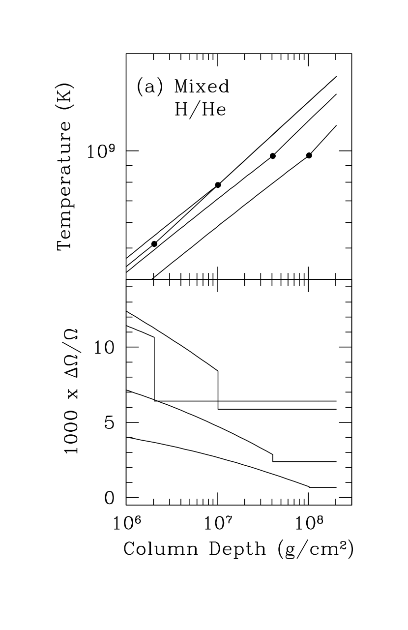
Figure 2.— Temperature profiles (upper panel) and spin down (lower panel) for the convective models of Table 3. In each case, the black dots mark the top of the convection zone at column depth $y_{c}$ (Table 3). (a) We show models for mixed H/He ignition with $\dot{m}=0.1\,\dot{m}_{\rm Edd}$, $Z_{\rm CNO}=0.01$, and $y_{b}=2.04\times 10^{8}\,{\rm g\,cm^{-2}}$. These models have $(y_{b}-y_{c})/y_{b}=0.5,0.8,0.95$ and $0.99$, $T_{b}/10^{9}\,{\rm K}=1.2,1.5,1.7$ and $1.7$, and $F/F_{\rm Edd}=0.31,0.74,1.15$ and $0.89$. (b) We show models for pure He ignition with $\dot{m}=0.015\,\dot{m}_{\rm Edd}$, $Z_{\rm CNO}=0.01$ and $y_{b}=2.53\times 10^{8}\,{\rm g\,cm^{-2}}$. These models have $(y_{b}-y_{c})/y_{b}=0.5,0.8,0.95$ and $0.99$, $T_{b}/10^{9}\,{\rm K}=1.3,1.6,1.95$ and $2.0$, and $F/F_{\rm Edd}=0.35,0.59,1.21$ and $1.06$. The difference in slope of the convective adiabat between models is due to the differing contribution of radiation pressure.

Figure 3.— Density as a function of height (solid lines) for the convective models of Table 3 and Figure 2 for (a) mixed H/He ignition and (b) pure He ignition. The density profile just before ignition is shown as a dashed line in each case. The black dots mark the height which encloses 90% of the mass. In (a) the density profiles of the two models with $F/F_{\rm Edd}=0.89$ and $1.15$ overlap.

Figure 4.— Temperature profiles (upper panel) and spin down (lower panel) for the fully-radiative models of Table 4. (a) We show constant flux models for mixed H/He ignition with $\dot{m}=0.1\,\dot{m}_{\rm Edd}$, $Z_{\rm CNO}=0.01$, and $y_{b}=2.04\times 10^{8}\,{\rm g\,cm^{-2}}$. These models have $F/F_{\rm Edd}=0.31,0.74$ and $1.15$ and $T_{b}/10^{9}\ {\rm K}=1.12,1.35$ and $1.49$. (b) We show constant flux models for pure He ignition with $\dot{m}=0.015\,\dot{m}_{\rm Edd}$, $Z_{\rm CNO}=0.01$, and $y_{b}=2.53\times 10^{8}\,{\rm g\,cm^{-2}}$. These models have $F/F_{\rm Edd}=0.35,0.59$ and $1.21$ and $T_{b}/10^{9}\ {\rm K}=1.19,1.34$ and $1.57$.

Figure 5.— Density as a function of height (solid lines) for the fully-radiative models of Table 4 and Figure 4 for (a) mixed H/He ignition and (b) pure He ignition. The density profile just before ignition is shown as a dashed line in each case. The black dots mark the height which encloses 90% of the mass.

Figure 6.— The $\Delta\Omega/\Omega$ profiles at different times as the convection zone shrinks, for mixed H/He ignition with $\dot{m}=0.1\dot{m}_{\rm Edd}$ and $Z_{\rm CNO}=0.01$. We take the initial extent of the convection zone to be $(y_{b}-y_{c})/y_{b}=0.8$ and the base temperature $T_{b}/10^{9}\,{\rm K}=1.5$. As the convection zone retreats, we assume the base temperature decreases linearly (eq. [21]) to $T_{b}/10^{9}\ {\rm K}=1.0$. We show $\Delta\Omega/\Omega$ as a function of depth for the initial model (80% of mass convective), an intermediate case (50%) and when the convective zone has almost vanished (5%). These models have $T_{b}/10^{9}\,{\rm K}=1.5,1.31,$ and $1.03$ and $F/F_{\rm Edd}=0.74,0.49,$ and $0.21$ respectively.

Figure 7.— Models of the cooling atmosphere in the tail of the burst. We show the physical thickness which encompasses 90% of the mass $\Delta z($90%$)$, as a function of the flux $F/F_{\rm Edd}$ for constant flux atmospheres. The solid curve is for the $\dot{m}=0.1\ \dot{m}_{\rm Edd}$, $Z_{\rm CNO}=0.01$ mixed H/He ignition model, where we take the composition to be pure ⁷³Kr. The dashed lines are for pure helium ignitions, $\dot{m}=0.01\ \dot{m}_{\rm Edd}$, $Z_{\rm CNO}=0.01$ (upper curve) and $\dot{m}=0.015\ \dot{m}_{\rm Edd}$, $Z_{\rm CNO}=0.01$ (lower curve). In this case, we take the composition to be ⁵⁶Ni. In each case, we show $\Delta z(90$%$)$ just before ignition by a horizontal solid line.

Figure 8.— Thermal time $t_{\rm therm}$ (eq.[22]) and wrap around time $\Delta\nu^{-1}$ for the convective models of Table 3. In each case, the solid line shows $t_{\rm therm}$, and the hatched region $\Delta\nu^{-1}$ for $\nu_{s}$=300–600 Hz. (a) Mixed H/He ignition convective models with (top to bottom) $F/F_{\rm Edd}=1.15,0.74$ and $0.31$. (b) Pure He ignition convective models with (top to bottom) $F/F_{\rm Edd}=1.21,0.59$ and $0.35$.

Figure 9.— Brunt-Väisälä frequency $N/2\pi$ and Richardson number ${\rm Ri}$ for (a) the fully-radiative, constant $F=0.74\ F_{\rm Edd}$ mixed H/He ignition model and (b) the fully-radiative, constant $F=0.59\ F_{\rm Edd}$ pure He ignition model. We show the total buoyancy by a solid line, the thermal buoyancy as a dotted line and the composition piece as a dashed line. The cross shows an estimate of $N/2\pi$ at the base, $N^{2}_{\rm base}=(g/H_{b})(\Delta\ln\mu)$, where we take the ashes as having $\mu=A/(1+Z)=2.1$. For the pure He ignition model (b), there is a peak in the buoyancy at the place where the hydrogen runs out ($y\approx y_{d}$), at this depth the composition piece of the buoyancy dominates the thermal piece.

Figure 10.— A section of the two-layer model. The burning layers and ashes are represented by layers of different constant density. The radial coordinate $z$ increases upwards, the transverse co-ordinate $y$ increases to the right. The vertical component of the rotation vector is $\Omega\cos\theta$, and the upper fluid (density $\rho_{+}<\rho_{-}$) is moving out of the page with velocity $R\Delta\Omega\sin\theta$. (a) The boundary between the two fluids (solid line) slopes because in the upper fluid there is horizontal pressure gradient which balances the Coriolis force (see text). (b) The nature of the baroclinic instability. If the fluid element is moved to point A, it is heavier than its surroundings, and experiences a restoring force. If it is moved to point B, however, it is heavier than its new surroundings but has dropped in the gravitational field, releasing energy. All motions within the so-called “wedge of instability” are convectively unstable in this way.

Figure 11.— Schematic of the evolution of the atmosphere during a burst for (a) mixed H/He ignition and (b) pure He ignition. The rapid energy release from helium burning reactions makes the initial stages of many bursts convective. After a time $\lesssim 1\ {\rm s}$ (see text for references to simulations of bursts), the convection zone shrinks and disappears, leaving a radiative atmosphere. For pure He ignition, the burst duration is typically $\approx 10\ {\rm s}$; for mixed H/He ignition, rp process H burning in the tail can prolong the burst for a further $\gtrsim 30\ {\rm s}$.

Figure 12.— The thickness of the atmosphere which contains 90% of the mass, $\Delta z(90$%$)$, as a function of the flux for constant flux radiative atmospheres (solid and dotted lines) and for the convective models of Table 3 (solid and open squares). For the radiative models, the upper curve is for composition profile the same as at ignition, while the lower curve is for a composition of ⁷³Kr (⁵⁶Ni) for the mixed H/He (pure He) case, chosen to represent the products of burning. Initially, the evolution of the thickness of the layer is along or above the upper curve as it ignites and heats up, depending on the extent of the convection zone. As nuclear burning proceeds, the mean molecular weight increases, and the thickness decreases, eventually moving back along the lower curve as the atmosphere cools. Just before ignition (upper curve, $F\ll F_{\rm Edd}$), the thickness of the accumulated layer is $\approx 5\ {\rm m}$. During the burst, the atmosphere expands hydrostatically by $\Delta z\approx 10$–$40\ {\rm m}$ ($\approx 5$–$20\ {\rm m}$). In the cooling tail, the thickness may differ by $\approx 1\ {\rm m}$ from that before the burst.

Figure 13.— The spin evolution of the atmosphere for convective (squares) and radiative (lines) models, assuming rigid rotation is maintained throughout the atmosphere. We plot the fractional spin frequency change of the burning shell, $\Delta\Omega/\Omega$, such that $\Delta\Omega/\Omega>0$ indicates spin down. As in Figure 12, the evolution during the burst is as shown by the arrows. We also indicate the observed frequency shifts for those objects listed in Table 1 by horizontal bars. For those bursts in which the oscillation frequency was seen only in the tail, we plot the $\Delta\Omega/\Omega$ value as a lower limit.

References

- (1) Ayasli, S., & Joss, P. C. 1982, ApJ, 256, 637
- (2) Benton, E. R., & Clark, A. 1974, Ann. Rev. Fluid Mech., 6, 257
- (3) Bhattacharya, D. 1995 in X-Ray Binaries, ed. W. H. G. Lewin, J. van Paradijs, & E. P. J. van den Heuvel (Cambridge: Cambridge University Press), 233
- (4) Bildsten, L. 1995, ApJ, 438, 852
- (5) Bildsten, L. 1998, in The Many Faces of Neutron Stars, ed. R. Buccheri, J. van Paradijs, & M. A. Alpar (Dordrecht: Kluwer), 419
- (6) Bildsten, L. 2000, in Cosmic Explosions, ed. S. S. Holt and W. W. Zhang (New York:AIP)
- (7) Bildsten, L., & Brown, E. F. 1997, ApJ, 477, 897
- (8) Bildsten, L., & Cumming, A. 1998, ApJ, 506, 842
- (9) Bildsten, L., & Cutler, C. 1995, ApJ, 449, 800
- (10) Bildsten, L., Ushomirsky, G., & Cutler, C. 1996, ApJ, 460, 827
- (11) Brekhovskikh, L. M., & Goncharov, V. 1994, Mechanics of Continua and Wave Dynamics (New York: Springer)
- (12) Brown, E. F., 2000, ApJ, 531, 988
- (13) Brown, E. F., & Bildsten, L. 1998 ApJ, 496, 915
- (14) Chakrabarty, D., & Morgan, E. H. 1998, Nature, 394, 346
- (15) Chandrasekhar, S. 1961, Hydrodynamic and Hydromagnetic Stability (New York:Dover)
- (16) Clayton, D. D. 1983, Principles of Stellar Evolution and Nucleosynthesis (Chicago: The University of Chicago Press)
- (17) Cox, J. P., & Giuli, R. T. 1968, Principles of Stellar Structure (New York: Gordon & Breach)
- (18) Dutton, J. A. 1995, Dynamics of Atmospheric Motion (New York: Dover)
- (19) Endal, A. S., & Sofia, S. 1978, ApJ, 220, 279
- (20) Fox, D. W., Muno, M. P., Morgan, E. H., & Bildsten L. 2000, in preparation
- (21) Fryxell, B. A., & Woosley, S. E. 1982, ApJ, 261, 332
- (22) Fujimoto, M. Y. 1988, A&A, 198, 163
- (23) Fujimoto, M. Y. 1993, ApJ, 419, 768
- (24) Fujimoto, M. Y., Hanawa, T., & Miyaji, S. 1981, ApJ, 247, 267 (FHM)
- (25) Fujimoto, M. Y., Sztajno, M., Lewin, W. H. G., & van Paradijs, J. 1987, ApJ, 319, 902
- (26) Fushiki, I., & Lamb, D. Q. 1987a, ApJ, 317, 368
- (27) Fushiki, I., & Lamb, D. Q. 1987b, ApJ, 323, L55
- (28) Greenspan, H. P., & Howard, L. N. 1963, J. Fluid Mech., 17, 385
- (29) Hanawa, T., & Fujimoto, M. Y. 1982, PASJ, 34, 495
- (30) Hanawa, T., & Fujimoto, M. Y. 1984, PASJ, 36, 199
- (31) Hanawa, T., & Sugimoto, D. 1982, PASJ, 34, 1
- (32) Hollingsworth, A. 1975, Quart. J. Roy. Meteorol. Soc., 101, 495
- (33) Hollingsworth, A., Simmons, A. J., & Hoskins, B. J. 1976, Quart. J. Roy. Meteo rol. Soc., 102, 901
- (34) Holton, J. R. 1965, J. Atmos. Sci., 22, 402
- (35) Hoyle, R., & Fowler, W. A. 1965, in Quasi-Stellar Sources and Gravitational Collapse, ed. I. Robinson, A. Schild, & E. L. Shucking (Chicago: University of Chicago Press)
- (36) Iben, I. Jr., 1991, in Evolution of Stars: The Photospheric Abundance Connection, ed. G. Michaud & A. Tutukov, 257
- (37) Joss, P. C. 1977, Nature, 270, 310
- (38) Joss, P. C. 1978, ApJ, 225, L123
- (39) Joss, P. C., & Li, F. K. 1980, ApJ, 238, 287
- (40) Knobloch, E., & Spruit, H. C. 1982, A&A, 113, 261
- (41) Koike, O., Hashimoto, M., Arai, K., & Wanajo, S. 1999, A&A, 342, 464
- (42) Kong, A. K. H., Homer, L., Kuulkers, E., Charles, P. A., & Smale, A. P. 2000, MNRAS, 311, 405
- (43) Langer, N., Heger, A., Wellstein, S., & Herwig, F. 1999, A&A, 346, L37
- (44) Lewin, W. H. G., van Paradijs, J., & Taam, R. E. 1995, in X-Ray Binaries, ed. W. H. G. Lewin, J. van Paradijs, & E. P. J. van den Heuvel (Cambridge: Cambridge University Press), 175
- (45) Livio, M., & Bath, G. T. 1982, A&A, 116, 286
- (46) Livio, M., & Truran, J. W. 1987, ApJ, 318, 316
- (47) Livio, M., & Truran, J. W. 1990, Ann. N. Y. Acad. Sci., 617, 126
- (48) McDermott, P. N., & Taam, R. E. 1987, ApJ, 318, 278
- (49) Miller, M. C. 1999, ApJ, 515, L77
- (50) Miller, M. C. 2000, ApJ, 531, 458
- (51) Moura, A. D., & Stone, P. H. 1976, J. Atmos. Sci., 33, 602
- (52) Muno, M. P., Fox, D. W., Morgan, E. H., & Bildsten L. 2000, Ap J, to appear
- (53) Nozakura, T., Ikeuchi, S., & Fujimoto, M. Y. 1984, ApJ, 286, 221
- (54) Paczynski, B. & Anderson, N. 1986, ApJ, 302, 1
- (55) Pedlosky, J. 1987, Geophysical Fluid Dynamics (New York: Springer)
- (56) Psaltis, D., & Chakrabarty, D. 1999, ApJ, 521, 332
- (57) Psaltis, D., & Lamb, F. K. 1998, in Neutron Stars and Pulsars, ed. N. Shibazaki, N. Kawai, S. Shibata, & T. Kifune (Tokyo: Univ. Acad. Press), 179
- (58) Sackmann, I.-J., & Boothroyd, A. I. 1991, in Evolution of Stars: The Photospheric Abundance Connection, ed. G. Michaud & A. Tutukov, 275
- (59) Sakurai, T., Clark, A. Jr., & Clark, P. A. 1971, J. Fluid Mech., 49, 753
- (60) Schatz, H., et al. 1998, Phys. Rep., 294, 167
- (61) Schatz, H., Bildsten, L., Cumming, A., & Wiescher, M. 1999, ApJ, 524, 1014
- (62) Schoelkopf, R. J., & Kelley, R. L. 1991, ApJ, 375, 696
- (63) Shapiro, S. L., & Teukolsky, S. A. 1983, Black Holes, White Dwarfs and Neutron Stars: The Physics of Compact Objects (New York:Wiley)
- (64) Shara, M. M. 1982, ApJ, 261, 649
- (65) Simmons, A. J., & Hoskins, B. J. 1976, J. Atmos. Sci., 33, 1454
- (66) Simmons, A. J., & Hoskins, B. J. 1977, J. Atmos. Sci., 34, 581
- (67) Smith, D. A., Morgan, E. H., & Bradt, H. 1997, ApJ, 479, L137
- (68) Spitzer, L. Jr. 1962, Physics of Fully Ionized Gases (2nd Ed.; New York: Wiley)
- (69) Spruit, H. C. 1999, A&A, 349, 189
- (70) Spruit, H. C., & Knobloch, E. 1984, A&A, 132, 89
- (71) Strohmayer, T. E. 1999a, ApJ, 523, L51
- (72) Strohmayer, T. E. 1999b, preprint (astro-ph/9911338)
- (73) Strohmayer, T. E., Jahoda, K., Giles, B. A., & Lee, U. 1997a, ApJ, 486, 355
- (74) Strohmayer, T. E., & Lee, U. 1996, ApJ, 467, 773
- (75) Strohmayer, T. E., & Markwardt, C. B. 1999, ApJ, 516, L81
- (76) Strohmayer, T. E., Swank, J. H., & Zhang, W. 1998a, Nucl. Phys. B (Proc. Suppl.), 69(1-3), 129
- (77) Strohmayer, T. E., Zhang, W., & Swank, J. H. 1997b, ApJ, 487, L77
- (78) Strohmayer, T. E., Zhang, W., Swank, J. H., & Lapidus, I. 1998b, ApJ, 503, L147
- (79) Strohmayer, T. E., Zhang, W., Swank, J. H., Smale, A., Titarchuk, L., Day, C., & Lee, U. 1996, ApJ, 469, L9
- (80) Strohmayer, T. E., Zhang, W., Swank, J. H., White, N. E., & Lapidus, I. 1998c, ApJ, 498, L135
- (81) Taam, R. E. 1980, ApJ, 241, 358
- (82) Taam, R. E., & Picklum, R. E. 1978, ApJ, 224, 210
- (83) Tassoul, J.-L., & Tassoul, M. 1982, ApJS, 49, 317
- (84) Truran, J. W. 1982, in Essays in Nuclear Astrophysics, ed. C. A. Barnes, D. D. Clayton, & D. Schramm (Cambridge: Cambridge University Press), 467
- (85) van der Klis, M. 2000, ARA&A, to appear September 2000 (astro-ph/0001167)
- (86) Walin, G. 1969, J. Fluid Mech., 36, 289
- (87) Wallace, R. K., & Woosley, S. E. 1981, ApJS, 45, 389
- (88) Wallace, R. K., Woosley, S. E., & Weaver, T. A. 1982, ApJ, 258, 696 (W82)
- (89) Warn, H. 1976, J. Atmos. Sci., 33, 1478
- (90) Wijnands, R., & van Der Klis, M. 1998, Nature, 394, 344
- (91) Zhang, W., Jahoda, K., Kelley, R. L., Strohmayer, T. E., Swank, J. H., & Zhang, S. N. 1998, ApJ, 495, L9
- (92)