CMB Cosmological Parameter Estimation: Methods and Current Results

The majority of present efforts to constrain cosmological parameters with cosmic microwave background (CMB) anisotropy data employ approximate likelihood functions, the time consuming nature of a complete analysis being a major obstacle. We have performed a full (unapproximated) likelihood analysis on several experiments that allows us to examine the various assumptions made in these approximate methods and to evaluate their performance. Our results indicate that care should be taken when using such approaches. With an improved approximate method, we present some constraints on cosmological parameters using the entire present CMB data set.

1 Introduction

Since their first detection by COBE, the CMB temperature fluctuations have become an essential tool for constraining cosmological parameters. The number of experiments measuring anisotropies at different scales is now close to 20. With time, the observations become more accurate and their angular resolution improves, increasing the number of pixels. This evolution towards higher precision measurements of CMB fluctuations inhibits complete (unapproximated) likelihood analyses over large sets of models (or free parameters). Approximate methods have thus been proposed in order to explore as much parameter space as possible with the complete CMB data set. Easy to use and fast, $\chi^{2}$ minimisation has been widely applied. The approximate nature of this method resides in two assumptions: (i) the one dimensional bandpower distribution is Gaussian; (ii) all pertinant information in a map is contained in the flat–band power. The latter is also assumed by other approximations, such as proposed by Bond et al. (1998), Wandelt et al. (1998) and Bartlett et al. (1999). Focussing on a small number of experiments (COBE, SASKATOON and MAX), we have performed a complete likelihood analysis over a reasonably representative set of (Inflationary) models. This allows us to compare our results with those from a $\chi^{2}$ minimisation and to quantitatively examine these two assumptions.

2 Testing the assumptions

In an inflationary scenario, the sky pixels are Gaussian distributed, and so also the $a_{lm}^{\prime}s$ in a spherical harmonic decomposition. But what is used in $\chi^{2}$ minimisation is the in–band power of the fluctuations; this corresponds to the square root of the temperature fluctuation variance and is not a Gaussian distributed quantity. This motivated us to look more carefully at the first assumption. Figure 1 shows an example where a 2-tailed Gaussian (with asymmetric errors; dot–dot–dashed line) is a rather bad approximation to the true likelihood curve (solid line). Even if the Gaussian appears relatively faithful near the maximum, it rapidly deviates from the likelihood function with the distance from the peak: the $\chi^{2}$ is thus very (overly) sensitive to the presence of outliers (which will be more common than it expects). By comparison, the approximation developed in Bartlett et al. (1999) reproduces quite well the likelihood function. More accurate (relative to a full likelihood treatment) parameter estimation can thus be obtained by using such approximate likelihood forms, or simply by direct interpolation of the one–dimensional in–band likelihood function, when available.

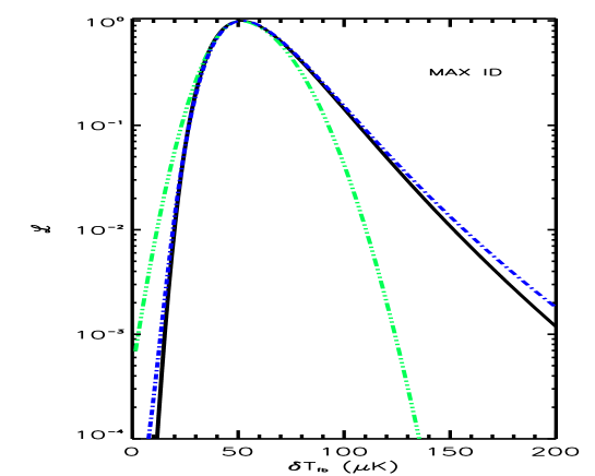
Figure 1: True likelihood (solid line), 2-tailed Gaussian (dot–dot–dashed) and our approximation (Bartlett et al. 1999, dot–dashed) for the MAX ID field.

The second assumption supposes that the flat–band power estimate contains all the information in a map. To check this assumption, we computed the flat–band power and its error bars for several bins of MAX and Saskatoon and will now compare the constraints suggested by these estimates to those from a full likelihood analysis. This is illustrated in Figure 2. By definition, models passing within the error bars are considered consistent with the flat–band estimates at the “one sigma confidence level”. This may be compared to the confidence level assigned by the full likelihood analysis: focussing on just the MAX PH point (at the extreme left in Figure 2–left), the likelihood analysis excludes the model plotted as the dotted line at more than 68%, but accepts the model shown as the dashed line, all in flagrent contradiction with the flat–band estimate. This can be understood by looking at Figure 2–right. Here, we show the results of a likelihood analysis over a family of spectra modeled by their in–band power ($\delta T_{N}$) and slope ($m$): $\delta T(\ell)=\delta T_{N}.(\ell/\ell_{eff})^{m}$. Figure 2–right displays likelihood contours in the plane ($\delta T_{N},m$) for MAX PH. We clearly see that MAX PH prefers spectra with positive slope and lower in–band power than the flat–band estimate (corresponding to the vertical line at m=0). The latter considers only the information available along the vertical line in Figure 2–right and looses signal contained in the rest of the plane. The symbols position the two models plotted in Figure 2–left, explaining the disagreement between the two analysis methods. The conclusion is that, at least in this example, the information contained in the original pixel set cannot be reduced to a flat–band estimate. In the case of MAX PH, any approximation using only the flat–band power will never result in the same constraints as a full likelihood analysis.

Incorporating all the information available in a map (in–band power, slope, …) will give more realistic constraints than possible with just flat–band estimates. A simple and efficient way to impliment this is by interpolation the likelihood surface over $\delta T_{N}$ and $m$ for each bin (instead of the one–dimensional curve for the flat–band power).

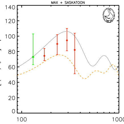
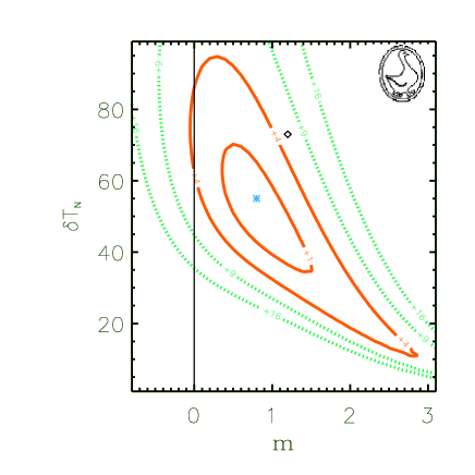
Figure 2: LEFT: Flat–band estimates for MAX PH and 4 bins of Saskatoon CAP. RIGHT: Likelihood contours over spectral power versus slope for MAX PH (see text). Flat–band power estimates are restricted to the vertical line.

3 Current Results

We took into account the above remarks in an attempt to obtain a more complete parameter estimation using the entire CMB data set and a large set of Inflationary models. In practice, we used our approximation for those experiments for which only the flat–band power estimate was given; interpolated the flat–band likelihood curve when it was available; and interpolated the likelihood surfaces (power, slope) of Saskatoon and MAX. Our analysis corresponds to 70 different data points representing 20 experiments, and more than 10 million models. The compute time required was 350 cpu–hours on a DEC workstation – equivalent to a simple $\chi^{2}$ minimisation.

Figures 3 show our principle results in the framework of open Inflationary models with a cosmological constant. The constraints are given as 2–dimensional (approximated) likelihood contours at roughly $68$ and $95\%$ confidence. In each case, the other investigated parameters $(H_{0},Q,n,\eta_{10})$ are marginalised by projection. A large number of the models are excluded in the plane $(\Omega_{k},\lambda_{0})$. Prefered models have very low curvature, although no the cosmological constant is relatively unconstrained. Figure 3–right is a nice summary of the status of the simplest of Inflationary predictions, namely that $n\sim 1$ and $\Omega_{k}=0$. These values are indeed favored by current CMB observations.

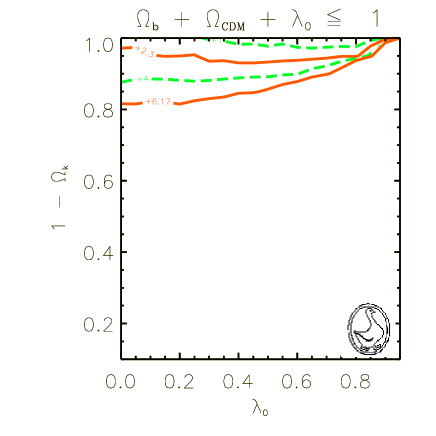
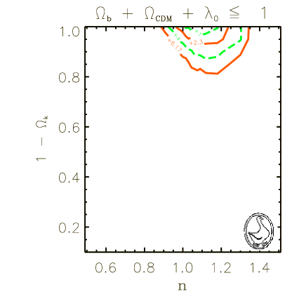
Figure 3: LEFT: Constraints in ($\Omega_{tot},\lambda_{0}$) plane obtained with our method. RIGHT: Constraints in in the ($\Omega_{tot},n$) plane.

4 Conclusion

We have seen how in some cases a Gaussian is a bad representation of the one–dimensional in–band power likelihood function. To improve on $\chi^{2}$ methods, we therefore recommend the use of other, more appropriate approximations, as proposed in the literature, or direct interpolation of the exact likelihood curve, when available. Even this may not be entirely satisfactory because flat–band power estimates do not always sufficiently represent a CMB data set. We have demonstrated that some of MAX and Saskatoon data (bins) prefer non–zero spectral slopes and different in–band powers. In these cases, the incorporation of additional information, for example, the in–band spectral slope, should lead to a better reproduction of the actual constraints. Taking these remarques into account, have also seen how the first generation experiments favor the simple Inflationary scenario predictions: curvature close to zero and spectral index close to one.

References

References

- [1] Bond J.R., Jaffe A.H. & Knox L. 1998, astro–ph/9808264
- [2] Bartlett J.G., Douspis M., Blanchard A. & Le Dour M. 1999, astro–ph/9903045
- [3] Douspis M., Bartlett J.G., Blanchard A. & Le Dour M. 2000, in preparation
- [4] Wandelt B. J., Hivon E. & Gorski K.M. 1998, astro–ph/9808292