Cosmological Constraints from the Cosmic Microwave Background

Abstract

Using an approximate likelihood method adapted to band–power estimates, we analyze the ensemble of first generation cosmic microwave background anisotropy experiments to deduce constraints over a six–dimensional parameter space describing Inflation–generated adiabatic, scalar fluctuations. The basic preferences of simple Inflation scenarios are consistent with the data set: flat geometries $(\Omega_{\rm tot}\equiv 1-\Omega_{\kappa}\sim 1)$ and a scale–invariant primeval spectrum ($n\sim 1$) are favored. Models with significant negative curvature ($\Omega_{\rm tot}<0.7$) are eliminated, while constraints on postive curvature are less stringent. Degeneracies among the parameters prevent independent determinations of the matter density $\Omega_{\rm m}$ and the cosmological constant $\Lambda$, and the Hubble constant $H_{\rm o}$ remains relatively unconstrained. We also find that the height of the first Doppler peak relative to the amplitude suggested by data at larger $l$ indicates a high baryon content ($\Omega_{\rm b}h^{2}$), almost independently of the other parameters. Besides the overall qualitative advance expected of the next generation experiments, their improved dipole calibrations will be particularly useful for constraining the peak height. Our analysis includes a Goodness–of–Fit statistic applicable to power estimates and which indicates that the maximum likelihood model provides an acceptable fit to the data set.

1 Introduction

The newest and perhaps most powerful tool in the cosmologist’s toolbox are the temperature fluctuations in the cosmic microwave background (CMB). Their very existence (e.g., Smoot et al. 1992) lends much credence to the general picture of gravitational instability forming galaxies and the observed large–scale structure. The last two decades have witnessed the elaboration of this idea, with numerical studies of gravitational growth permitting quantitative comparison to actual survey data, and with the introduction of a physical mechanism – namely, Inflation – for the creation of the initial perturbations. Daring in scope, the resulting scenario would encompass the evolution of the Universe from possibly the Planck era to the present, explaining not only the origin of the required density perturbations, but also dispelling a handful of misgivings about the initial conditions of Big Bang model, such as the impressive homogeneity on large scales (Kolb & Turner 1990; Peebles 1993; Peacock 1999) Like any theory, it can never be proved; but it may be tested. And like any good theory, it provides a physics, dependent on the validity of the theory, specific enough to be used as a tool to other ends: it is now well appreciated that detailed study of the CMB fluctuations may be applied to determine the fundamental parameters of the Big Bang model itself (Bond et al. 1994; Knox 1995; Jungmann et al. 1996).

Our object with the present study is to examine what may be learned from present CMB data within the Inflationary context. It should be noted at the outset that there are other models contending to explain the origin of density perturbations, for example, defect models (Durrer 1999). Neither these nor any other alternative shall be our concern in the following, and it is important to emphasize that our results are therefore limited to the Inflationary context. Very specifically, we shall be concerned only with temperature fluctuations caused by adiabatic, coherent and passively evolving density (scalar) perturbations, dominated by cold dark matter (CDM) (Bond & Efstathiou 1984; Vittorio & Silk 1984). Inflation can generate isocurvature modes, but we ignore these in the following, along with gravitational waves, the only non–scalar modes expected in Inflationary scenarios, and reionization. All model predictions have been calculated using the CAMB Boltzmann code developed by Lewis, Challinor & Lasenby (1999) and built upon CMBFAST (Seljak & Zaldarriaga 1996; Zaldarriaga, Seljak & Bertschinger 1998) The reason for these restrictions is of course that it is impossible to explore the otherwise vast parameter space.

Even in this seemingly restrained setting, the physics of CMB temperature anisotropies is quite rich, but it may nevertheless be boiled down to two regimes: large scales where purely gravitational effects operate [Sachs–Wolfe (SW) effect; Sachs & Wolfe 1967], and small scales, within the horizon at recombination where causal physics plays its role. In the latter regime, pressure of the coupled baryon–photon fluid resists the inward pull of gravity and therein establishes oscillating sound waves that will be observed in the CMB fluctuation power spectrum as a sequence of power peaks (so–called Doppler peaks; e.g., Hu & Sugiyama 1996). These are damped towards the smallest scales by smoothing due to the finite thickness of the last scattering surface from which emanates the CMB. The well defined aspect of these power peaks owes to the coherent nature and passive evolution of Inflation generated perturbations; the loss of both of these in defect models has the effect of broadening or completely smearing out the peaks (see, e.g,. Durrer 1999 and references therein). The very existence of such a series of power peaks is thus a strong discriminator between models.

Besides the exact details of the physics of Inflation, the development of such perturbations depends, unsurprisingly, on the constituents of the primordial plasma in which they reside, as well as on the metric background in which they evolve. This provides the link between the observable sky temperature fluctuations and the fundamental cosmological parameters. Actual data from the first generation of CMB experiments already indicates the existence of the first Doppler peak, a fact that leads to interesting and non–trivial conclusions, as noted by many authors and as detailed below.

In this paper we present our constraints over a six–dimensional parameter space (see Table 1) resulting from a large compilation of first generation experiments (see Table 2). Our conclusions are based not on a traditional $\chi^{2}$ approach, but on methods developed and presented elsewhere which attempt to account for the non–Gaussian nature of power spectrum estimates as well as information at times lost in simple band–power estimates [Bartlett et al. 1999 (BDBL); Douspis et al. 2000 (DBBL); Douspis, Bartlett & Blanchard (DBB)]; we have tested these methods against complete likelihood analyses over subsets of the present CMB data. Our parameter space here is spanned by the quantities listed in Table 1, namely, the Hubble constant $H_{\rm o}$; the total energy density $\Omega_{\rm tot}\equiv\Omega_{\rm m}+\lambda_{\rm o}$, where $\Omega_{\rm m}$ is the matter density and $\lambda_{\rm o}\equiv\Lambda/3$; the vacuum energy density parameter $\lambda_{\rm o}$; the baryon density, $\Omega_{\rm b}$, in terms of $\eta_{10}\equiv$ (baryon–to–photon number ratio)$\times 10^{10}$ ($\Omega_{\rm b}h^{2}=0.00366\eta_{10}$); and the primordial scalar spectral parameters $n$ and $Q$, i.e., the slope and normalization. Our data set is listed in detail in Table 2.

While some recent analyses have covered a larger parameter space (e.g., Tegmark & Zaldarriaga 2000), they are based on traditional $\chi$–squared methods. In a key work, Dodelson & Knox (1999) applied approximate likelihood methods similar to those employed here, although over a more restricted range of parameters. The present work thus extends the approximate likelihood approach to a larger parameter space and includes an appropriate GoF statistic. On the other hand, we have not considered the effects of calibration uncertainties; the agreement between our results and those of previous authors supports the idea that these do not make a drastic difference to the final conclusions.

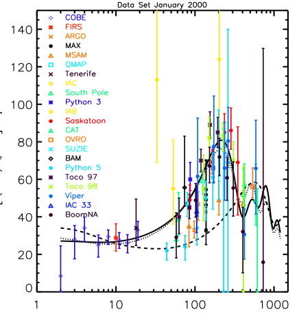
Figure 1: The power plane: measured flat–band power estimates and model spectra as a function of multipole. The solid line shows our best fit model (by approximate maximum likelihood) excluding the Python V points (see text): $(H_{\rm o},\Omega_{\rm tot},\lambda_{\rm o},\Omega_{\rm b}h^{2},n,Q)=(60\;$km/s/Mpc,$1.0,0.3,0.032,1.06,16.0\;\mu$K). Our GoF statistic indicates that this is an acceptable fit. We also plot as the dotted line the best model with with a fixed $\Omega_{\rm b}h^{2}=0.011$, falling $2\sigma$ below the prefered value: $(H_{\rm o},\Omega_{\rm tot},\lambda_{\rm o},\Omega_{\rm b}h^{2},n,Q)=(50\;$km/s/Mpc,$1.1,0.8,0.011,1.00,19.0\;\mu$K). The dashed line is an open model with $\Omega_{\rm tot}=0.2$ and $H_{\rm o}=60$ km/s/Mpc, shown for illustration and clearly excluded by the data.

The paper develops as follows: we begin in the next section with a presentation of our analysis methods; for the most part, this is a brief review of work presented in BDBL, DBBL and DBB. Our parameter constraints are then given in Section 3, followed by our conclusions in Section 4. The basic and robust result at this stage must be considered as the conclusion that the spatial curvature is close to zero and the primordial spectral index close to its scale–invariant value of unity. The results of our adapted statistical analysis are thus in agreement with many others (Lineweaver et al. 1997; Bartlett et al. 1998ab; Bond & Jaffe 1998; Efstathiou et al. 1998; Hancock et al. 1998; Lahav & Bridle 1998; Lineweaver & Barbosa 1998ab; Lineweaver 1998; Webster et al. 1998; Lasenby et al. 1998; Dodelson & Knox 1999; Melchiorri et al. 1999; Tegmark & Zaldarriaga 2000; Knox & Page 2000) and confirm the two fundamental predictions of the Inflationary model.

2 Analysis Method

The experimental results of Table 2 are shown in Figure 1 as standard band–power estimates, together with several theoretical curves. As for most current analyses, this will be our starting point. Simple as it may at first appear, a correct statistical approach to these data is in fact a non–trivial issue. The temptation is of course to apply a traditional $\chi^{2}$ minimization to the ensemble of points and errors. This, however, is not strictly allowed, for these points, being power estimates, are not Gaussian distributed. In addition, the given errors are usually computed from the the band–power likelihood function and do not therefore necessarily represent the errors on the power estimate (which a frequentist would argue must be found by simulation). In general, the best statistical method to constrain parameters with CMB data would be a likelihood analysis based on the original pixel values (or temperature differences; in this paper, we use the term ‘pixel’ to refer to differences as well), because this is guaranteed to use all relevant experimental information. Straightforward to construct in the (present) context of Gaussian theories as a multi–variant Gaussian in the pixel values, whose covariance matrix depends on the underlying model parameters (and noise characteristics), the likelihood is in practice computationally cumbersome due to the required matrix operations (Bond, Jaffe & Knox 1998; Borrill 1999ab; Kogut 1999).

	$H_{\rm o}$ (km/s/Mpc)	$\Omega_{\rm tot}$	$\lambda_{\rm o}$	$\eta_{10}$	$n$	$Q\;\mu$K
Min.	20	0.1	0.0	1.11	0.70	10.0
Max.	100	2.0	1.0	10.66	1.42	25.0
step	10	0.1	0.1	1.91	0.06	1.5

Table 1: Parameter space explored:

$\Omega_{\rm tot}\equiv 1-\Omega_{\kappa}$, where $\Omega_{\kappa}$ is the curvature parameter
$\lambda_{\rm o}\equiv\Lambda/3$
$\eta_{10}\equiv$ (baryon number density)/(photon number density)
         $\times 10^{10}$    (Note: $\Omega_{\rm b}h^{2}=0.00366\eta_{10}$)
$n\equiv$ primeval spectral index
$Q\equiv\sqrt{(5/4\pi)C_{2}}$

This difficulty has motivated us (BDBL; DBBL; DBB) and others (Bond, Jaffe & Knox 1998; Wandelt, Hivon & Górski 1998) to propose methods based on power estimates and aimed at reproducing as far as possible a complete likelihood analysis. Computation time is greatly reduced by working in the power plane (Bond, Jaffe & Knox 1998; Tegmark 1997), due to the much smaller number of data elements, but all proposed methods must be benched against the ultimate goal of recovering the likelihood results. In DBBL we evaluated at length the viability of several approximate methods by comparison to a complete likelihood analysis. We found that the traditional $\chi^{2}$ method over power estimates (such as shown in Figure 1) is subject to bias. Other approaches based on approximate band–power likelihood functions fare better, but still do not always fully reproduce the complete likelihood results. As discussed in DBBL, this may be traced to relevant experimental information lost by the simple band–power representation of an experiment; we demonstrated this explicitly by showing that some MAX and Saskatoon data are sensitive to the local slope of the power spectrum. In other words, the observations constrain not only an in–band power, but also a local effective spectral slope. This information is correctly incorporated by a complete likelihood analysis, but obviously missed by any method based solely on the band–power estimates of Figure 1.

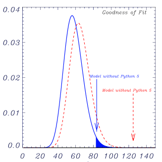
Figure 2: GoF statistic: shown are the distribution and observed value of our generalized $\chi^{2}$ for the fit without Python V (blue, solid distribution and arrow), and for the fit including the Python V points (dashed, red distribution and arrow). The fit is reasonable in the former case, but unacceptable in the latter (see text).

These comments motivate an approach in which all relevant experimental information is first identified by a set of parameters that are constrained by the data. A general likelihood function may then be constructed over this parameter space using the original pixel set; this need be done only once. Expressing a general power spectrum by these same parameters then permits one to assign a likelihood value to any model by extrapolation of the pre–calculated likelihood function. This value incorporates all pertinent information and should be the best possible approximation to the exact likelihood. The gain is that one manipulates the likelihood function with the full pixel set only once, and then simply interpolates over a much reduced set of parameters. Once the likelihood function has been calculated, the technique is hardly more complicated than the traditional $\chi^{2}$ employed for its facility. Unfortunately, the information needed for a general application of this technique to all of the current experimental results is not readily available. Because the number of points we are able to treat in this fashion is thus small, we elect to analyze the entire data set with the band–power approximation developed in BDBL.

We examine a set of Inflationary models over the parameter space spanned by $(H_{\rm o},\Omega_{\rm tot},\lambda_{\rm o},\eta_{10},n,Q)$, with respective ranges and step sizes given in Table 1. The likelihood of each model is calculated as just described, and the best model is found by maximizing the likelihood function over the explored space. We present our results as a series of two–dimensional contour plots of the likelihood projected onto various parameter planes. The contours are defined in the full six–dimensional space with values of $\Delta\log({\cal L})=1,4$ (dashed, in green), motivated as the 1 and 2 $\sigma$ contours of a Gaussian distribution when projected onto one of the axes, and of $\Delta\log({\cal L})=2.3,6.17$ (solid, in red), motivated by a Gaussian distribution with two degrees of freedom. Since the likelihood is not actually Gaussian, the confidence percentages associated with our contours are not exactly 1 and 2 “$\sigma$”; the technique is however standard practice. Our final results shown in the following figures have been obtained by excluding the Python V points. As discussed below, this is because the inclusion of this data set leads to a poor GoFfor the entire class of models considered. On formal grounds we would then be lead to reject the models, while on a technical note we worry that likelihood contours for a poor best–fit may give misleading constraints. Perhaps somewhat arbitrarly, we thus proceed in our analysis without these data. This difficulty would in part be alleviated by a complete treatment of calibration errors.

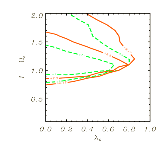
Figure 3: Constraints in the $(\Omega_{\rm tot},\lambda_{\rm o})$–plane, where the other parameters have been projected out; $1=\Omega_{\rm tot}+\Omega_{\kappa}=\Omega_{\rm m}+\lambda_{\rm o}+\Omega_{\kappa}$, and $\lambda_{\rm o}\equiv\Lambda/3$. Hyperbolic models are strongly ruled out, but the constraints are less stringent on spherical geometries. The degeneracy between $\Omega_{\rm m}$ and $\lambda_{\rm o}$ preventing independent determinations of the matter and vacuum contributions is manifest as the horizontal orientation of the contours.

Another aspect of our analysis not incorporated, as far as we are aware, in previous work is the application of an adequate goodness–of–fit statistic (GoF). Once the best model, i.e., the most likely model, has been found, one is obliged to evaluate the quality of its description of the data. As for the likelihood function itself, our situation is complicated by the fact that the power estimates shown in Figure 1 are not Gaussian distributed variables; in particular, a traditional $\chi^{2}$ GoF statistic is inadequate for the task. In DBB we proposed a GoF statistic readily applicable, if necessarily approximate, to band–power estimates. One requires distribution of these power estimates, $\hat{\delta T_{\rm fb}}$, for a given, underlying model; this distribution is not the same as the band–power likelihood function (frequentist point–of–view). Remarkably, we found in DBB that the same parameters introduced in BDBL to approximate the band–power likelihood function could be re–employed in a slightly different fashion to yield the distribution of the power estimator. The technique was tested with Monte Carlo simulations of experiments for which we performed complete likelihood analyses; details may be found in DBB. The important point is that with just the best power estimate and a confidence interval, we may construct an approximation to the complete distribution of the power estimate from an experiment and, hence, a GoF statistic for the data ensemble shown in Figure 1.

3 Results

Although perhaps at first glance the observational situation shown in Figure 1 seems confused, in fact the first Doppler peak would appear clearly detected. Several different experiments viewing different regions of sky on this scale, such as BOOMERanG, Python V, Saskatoon, Toco and QMAP, all indicate the presence of a rise in power and, in some cases, a hint of the subsequent fall–off, which is also supported by other experiments at higher $l$. This is not to say that all the data follow exactly the same party line, one example being the rather low MSAM points around the peak, but one could argue that the general trend favors the presence of a rise in power over the scales expected for first Doppler peak of Inflationary scenarios.

The way to quantify these statements is by fitting a model to the data and examining its GoF statistic. Over the parameter space explored and excluding the Python V points for the moment, the data identify the model with $(H_{\rm o},\Omega_{\rm tot},\lambda_{\rm o},\Omega_{\rm b}h^{2},n,Q)=(60\;{\rm km/s/Mpc},1.0,0.3,0.032,1.06,16.0\;\mu{\rm K})$ as the best fit; the corresponding model spectrum is shown in Figure 1 as the solid curve. The quality of the fit may be judged from the distribution of our GoF statistic (referred to as a generalized $\chi^{2}_{\rm gen}$) as shown in Figure 2. Assuming the data come from the adopted model, a value of $\chi^{2}_{\rm gen}$ as big or larger than the observed value (indicated by the heavy arrow) occurs with a probability of 0.014 (i.e., 1.4% of the time; indicated by the shaded area under the curve). Admittedly, this is a little low, but it does give a rather satisfying numerical representation of the impression given by the data (it seems reasonable). Although perhaps the fit is marginal, we certainly do not find the result sufficiently conclusive to eliminate the entire class of models from consideration. We are further comforted in this direction by the fact that the GoF is dominated by only a few outliers (see DBB). We thus do not hesitate to accept the model and move on to see what constraints the data provide over the parameter space considered. We remark in passing that a (incorrect) standard $\chi^{2}$ statistic is even less kind to the model with a value only 0.0016 (i.e., 0.16%) probable. Keeping the Python V points in the analysis yields a very poor best–fit model, quantified by a value of $\chi^{2}_{\rm gen}$ only $2\times 10^{-5}$ probable (marked on the figure by the dashed (green) curve and arrow). This is the reason for which we choose to exclude Python V in the following; thus, all our final results quoted hereafter and shown in the figures exclude this data set. Fully aware that such a procedure should always be undertaken only with caution (perhaps the fluctuations are not Gaussian, for example), we nevertheless feel that this is the most constructive approach at present. In some sense this is a purely formal argument, but we do worry about the interpretation of the contours from a likelihood with a poor GoF. In any case, the best–fit model is only slightly changed by inclusion of Python V: $(H_{\rm o},\Omega_{\rm tot},\lambda_{\rm o},\Omega_{\rm b}h^{2},n,Q)=(60\;{\rm km/s/Mpc},1.0,0.5,0.032,1.12,13.0\;\mu{\rm K})$. For comparison, we also calculated the GoF for the so–called “concordance model” $(H_{\rm o},\Omega_{\rm tot},\lambda_{\rm o},\Omega_{\rm b}h^{2},n,Q)=(65\;{\rm km/s/Mpc},1.0,0.3,0.018,1,20.0\;\mu{\rm K})$: we find a GoF 0.1% probable.

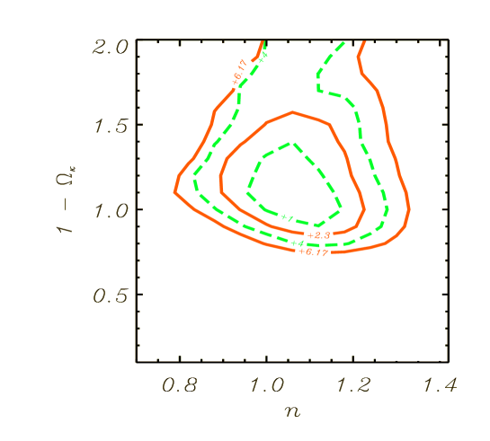
Figure 4: Constraints in the $(\Omega_{\rm tot},n)$–plane. We see that the fundamental expectations of simple Inflation models remain consistent with the data, namely, a flat geometry ($\Omega_{\kappa}\sim 0$) and a scale–invariant, primeval density perturbation power spectrum ($n\sim 1$).

The presence of the first Doppler peak in the data permits the elaboration of non–trivial constraints over our parameter space. Within our present context of adiabatic Inflation–generated perturbations, this peak appears on the physical scale of the horizon at the moment of recombination, $\sim H_{\rm o}^{-1}\sqrt{\Omega_{\rm m}}$. As the distance to the last scattering surface is also proportional to $H_{\rm o}^{-1}$ ($D_{\rm a}=H_{\rm o}^{-1}d_{\rm a}(\Omega_{\rm m},\lambda_{\rm o})$) the Hubble constant has relatively little influence on the projected angular scale of the peak; rather, $\Omega_{\rm m}$ and, most notably, the curvature of space (light ray focusing) control this observable scale (Blanchard 1984). For this reason, one should expect that the most robust result coming out of the present data set would be constraints in the $(\Omega_{\rm tot},\lambda_{\rm o})$–plane, as shown in Figure 3. The remarkable conclusion is that a flat universe is prefered and that, in particular, models with negative curvature (low $\Omega_{\rm tot}$) are eliminated. On the other hand, the data place only weak constraints on the value of the cosmological constant. This degeneracy between $\Omega_{\rm m}$ and $\lambda_{\rm o}$ is consistent with the expectation that one constrains instead their combination defining the quantity $\sqrt{\Omega_{\rm m}}/d_{\rm a}(\Omega_{\rm m},\lambda_{\rm o})$.

If spatial flatness may be considered as one of the motivating principals and a key “prediction” of the overall Inflation paradigm, then another is certainly the form of the primordial density perturbation spectrum, $n$. Figure 4 shows our constraints in the $(\Omega_{\rm tot},n)$–plane. The two most simple “predictions” of Inflation are rapidly evaluated on this diagram, and we see that the model fares quite well: zero spatial curvature ($\Omega_{\rm tot}=1-\Omega_{\kappa}=1$) and the spectral index of a scale–invariant spectrum ($n=1$) both fall within the inner contour.

As already mentioned, the best–fit model appears acceptable (marginally) according to our GoF statistic. Since our statistic is based on the assumption of Gaussianity, this in particular implies that the data are consistent with Gaussian anisotropies, as also expected in the simplest Inflationary scenarios. The general, overall conclusion from the first generation CMB anisotropy experiments must then be their coherence with the rudimentary concepts of Inflation.

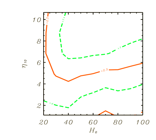
Figure 5: Constraints in the $(\eta_{10},H_{\rm o})$–plane. We find that high values of $\eta_{10}$ are favored by the present data set (see text). This appears to be primarily due to the height of the first Doppler peak and to the fact that some data (e.g., BOOMERanG N.A. and Viper) indicate a rapid fall–off before the second Doppler peak. For illustration, we also plot in Figure 1 a model with $\eta_{10}=3.0$ (other parameters chosen to maximize the likelihood for this value of $\eta_{10}$). Note that the low D/H abundances in some QSO systems would correspond to $\eta_{10}=5$ (Tytler et al. 2000).

One surprise of our analysis concerns the baryon density, $\Omega_{\rm b}$. As seen in Figure 5, the data indicate extremely high values of $\Omega_{\rm b}h^{2}$, and this almost independently of the value of the other parameters. So–called low D/H values observed in some QSO absorption systems yield $\eta_{10}\sim 5$ (Tytler et al. 2000), while here the CMB data prefer even higher baryon densities; although within “$2\sigma$” the two remain consistent. We believe the origin of this result to be related to the relative height of the first Doppler peak. Some data, such as Toco 97 & 98 and Saskatoon, suggest a high peak followed by a deep trough; low power at higher $l$ is also supported by other experiments, like Viper. For illustration, we show as the dotted line in Figure 1 the best–fit model with a fixed $\Omega_{\rm b}h^{2}=0.011$. The essential differences between this model and the overall best–fit model are (in the fomer case) a lower first peak and the absence of a deep trough before the appearance of the second peak. One important aspect (besides the anticipated large improvement in overall data quality) of the next generation mapping experiments (e.g., Archeops, BOOMERanG, and MAXIMA) is their ability to calibrate on the CMB dipole. This new calibration method, plus the fact that the entire first peak will be covered by a single instrument, should help to reduce the uncertainty surrounding the peak heights. As we have just argued, this is particularly important for determination of such quantities as the baryon density, and it will be an important test of the present result favoring a high baryon density.

4 Conclusions

Our purpose in this paper has been to analyze the ensemble of first generation CMB anisotropy experiments to see what conclusions may be drawn concerning certain fundamental cosmological parameters from the CMB data alone. Our approach employs approximate likelihood methods that are adapted to power estimates, and which have been detailed elsewhere (BDBL, DBBL and DBB). Our primary conclusions are that a flat geometry ($\Omega_{\kappa}\sim 0$ or $\Omega_{\rm tot}\sim 1$) and a scale–invariant primeval spectrum ($n\sim 1$) are favored, while strongly hyperbolic models are ruled out with high significance – in short, Inflation remains a good theory. Specifically, the best–fit model parameters are $(H_{\rm o},\Omega_{\rm tot},\lambda_{\rm o},\Omega_{\rm b}h^{2},n,Q)=(60\;{\rm km/s/Mpc},1.0,0.3,0.032,1.06,16.0\;\mu{\rm K})$. Our analysis includes a GoF statistic that indicates that this model, and therefore the entire class (Inflation with adiabatic, scalar perturbations and without re–ionization) provides an acceptable description of the data. Many authors have recently explored these issues (Lineweaver et al. 1997; Bartlett et al. 1998ab; Bond & Jaffe 1998; Efstathiou et al. 1998; Hancock et al. 1998; Lahav & Bridle 1998; Lineweaver & Barbosa 1998ab; Lineweaver 1998; Webster et al. 1998; Lasenby et al. 1998; Dodelson & Knox 1999; Melchiorri et al. 1999; Tegmark & Zaldarriaga 2000; Knox & Page 2000), with various combinations of the present data set, and most would agree with these conclusions. The extensive spectral coverage (in multipole order $l$) over the first, and perhaps second Doppler peaks, and the low noise expected of the next generation instruments should qualitatively change the confidence in and precision of this kind of study.

Very little may be said about $H_{\rm o}$ or about the relative contributions of matter, $\Omega_{\rm m}$, and vacuum, $\lambda_{\rm o}$, to the total energy density, the latter due to a well–known degeneracy when considering CMB data alone. One must turn to other observational constraints, coming from, for example, cluster evolution (Oukbir & Blanchard 1992), cluster baryon fractions (White et al. 1993), SNIa Hubble diagrams (Reiss et al. 1998; Perlmutter et al. 1999), weak cosmic shear (Blandford et al. 1991; Mellier 1999), etc…, to eliminate such degeneracies (so–called “cosmic complementarity”, Eisenstein, Hu & Tegmark 1999). Many of the authors listed above have included such constraints in their analysis; our own work along these lines is left to a forthcoming paper.

A surprising note is the very high baryon densities that we have found are prefered by the data set: $\eta_{10}\sim 8.9$ or $\Omega_{\rm b}h^{2}\sim 0.032$. This is even higher than the values indicated by the “low” D/H values found in several QSO absorption systems (Tytler et al. 2000), although within “$2\sigma$” (a little more for high values if $H_{\rm o}$; see Figure 5) the results are consistent. It remains to be seen if this intriguing result bears the scrutiny of the next generation experiments. In particular, their ability to significantly reduce overall calibration uncertainty by using the CMB dipole will be crucial to such issues.

Experiment	$\delta T\pm\sigma(\mu K)$	$\ell_{eff}$	reference
ARGO 1	$32.9^{+4.8}_{-4.1}$	98	Ratra et al. 1999
ARGO 2	$46.7^{+9.5}_{-12.1}$	98	Masi et al. 1996
BAM	$55.6^{+27.4}_{-9.8}$	74	Tucker et al. 1997
BOOM NA	$29.1^{+13.0}_{-11.0}$	58	Mauskopf et al. 1999
BOOM NA	$48.8^{+9.0}_{-9.0}$	102	Mauskopf et al. 1999
BOOM NA	$67.1^{+10.0}_{-9.0}$	153	Mauskopf et al. 1999
BOOM NA	$71.9^{+10.0}_{-10.0}$	204	Mauskopf et al. 1999
BOOM NA	$60.8^{+11.0}_{-12.0}$	255	Mauskopf et al. 1999
BOOM NA	$55.4^{+14.0}_{-15.0}$	305	Mauskopf et al. 1999
BOOM NA	$32.1^{+13.0}_{-22.0}$	403	Mauskopf et al. 1999
BOOM NA	$15.8^{+114.}_{-15.8}$	729	Mauskopf et al. 1999
CAT 1a	$51.8^{+13.6}_{-13.6}$	410	Scott et al. 1996
CAT 1b	$49.1^{+19.1}_{-13.6}$	590	Scott et al. 1996
CAT 2a	$57.3^{+11.}_{-13.6}$	422	Baker et al. 1997
CAT 2b	$0.0^{+55.0}_{-0.0}$	615	Baker et al. 1997
COBE 1	$8.5^{+16.}_{-8.5}$	2	Tegmark & Hamilton 1997
COBE 2	$28.0^{+7.4}_{-10.4}$	3	Tegmark & Hamilton 1997
COBE 3	$34.0^{+5.9}_{-7.2}$	4	Tegmark & Hamilton 1997
COBE 4	$25.1^{+5.2}_{-6.6}$	6	Tegmark & Hamilton 1997
COBE 5	$29.4^{+3.6}_{-4.1}$	8	Tegmark & Hamilton 1997
COBE 6	$27.7^{+3.9}_{-4.5}$	11	Tegmark & Hamilton 1997
COBE 7	$26.1^{+4.4}_{-5.3}$	14	Tegmark & Hamilton 1997
COBE 8	$33.0^{+4.6}_{-5.4}$	19	Tegmark & Hamilton 1997
FIRS	$29.4^{+7.8}_{-7.7}$	10	Ganga et al. 1994
IAB	$124.0^{+60.}_{-60.}$	203	Piccirillo et al. 1993
IAC 1	$113.0^{+49.}_{-44.}$	33	Femenia 1998
IAC 2	$55.0^{+27.}_{-28.}$	53	Femenia 1998
IAC 33	$43.0^{+12.5}_{-11.5}$	105	Dicker et al. 1999
MAX GUM	$54.5^{+16.4}_{-10.9}$	138	Tanaka et al. 1996
MAX HR	$27.9^{+11.5}_{-4.7}$	130	Our analysis
MAX ID	$52.7^{+32.1}_{-10.4}$	120	Our analysis
MAX PH	$72.9^{+30.6}_{-10.7}$	131	Our analysis
MAX SH	$82.0^{+53.0}_{-15.0}$	121	Our analysis
MSAM 1	$35.0^{+15.0}_{-11.0}$	84	Wilson et al. 2000
MSAM 1	$49.0^{+10.0}_{-8.0}$	201	Wison et al. 2000
MSAM 1	$47.0^{+7.0}_{-6.0}$	407	Wilson et al. 2000
OVRO	$56.1^{+8.5}_{-6.6}$	537	Leitch et al. 2000
Pyth A	$60.0^{+9.0}_{-5.0}$	87	Platt et al. 1997
Pyth B	$66.0^{+11.}_{-9.0}$	170	Platt et al. 1997
Python V	$22.0^{+4.0}_{-5.0}$	44	Coble 1999 thesis
Python V	$24.0^{+6.0}_{-7.0}$	75	Coble 1999 thesis
Python V	$34.0^{+7.0}_{-9.0}$	106	Coble 1999 thesis
Python V	$50.0^{+9.0}_{-12.0}$	137	Coble 1999 thesis
Python V	$61.0^{+13.0}_{-17.0}$	168	Coble 1999 thesis
Python V	$77.0^{+20.0}_{-28.0}$	199	Coble 1999 thesis
Python V	$69.0^{+71.0}_{-69.0}$	261	Coble 1999 thesis
Python V	$0.0^{+87.0}_{-0.0}$	230	Coble 1999 thesis
QMap,K1	$47.0^{+6.0}_{-7.0}$	80	de Oliveira-Costa 1998
QMap,K2	$59.0^{+6.0}_{-7.0}$	126	de Oliveira-Costa 1998
Sask 1	$51.5^{+8.4}_{-5.3}$	86	Netterfield et al. 1997
Sask 2	$72.5^{+7.4}_{-6.3}$	166	Netterfield et al. 1997
Sask 3	$89.3^{+10.5}_{-8.4}$	236	Netterfield et al. 1997
Sask 4	$90.3^{+12.6}_{-10.5}$	285	Netterfield et al. 1997
Sask 5	$72.5^{+20.}_{-29.4}$	348	Netterfield et al. 1997
SP91	$28.0^{+9.5}_{-6.7}$	58	Gundersen et al. 1995
SP94	$36.3^{+13.6}_{-6.1}$	62	Gundersen et al. 1995
SuZIE	$0.0^{+44.0}_{-0.0}$	2340	Ganga et al. 1997
Tenerife	$34.0^{+15.5}_{-9.3}$	18	Gutiérrez et al. 2000

Experiment	$\delta T\pm\sigma(\mu K)$	$\ell_{eff}$	reference
Toco 97	$40.0^{+10.0}_{-9.0}$	63	Torbet et al. 1999
Toco 97	$45.0^{+7.0}_{-6.0}$	85	Torbet et al. 1999
Toco 97	$70.0^{+6.0}_{-6.0}$	119	Torbet et al. 1999
Toco 97	$89.0^{+7.0}_{-7.0}$	155	Torbet et al. 1999
Toco 97	$85.0^{+8.0}_{-8.0}$	194	Torbet et al. 1999
Toco 98	$55.0^{+18.0}_{-17.0}$	128	Miller et al. 1999
Toco 98	$82.0^{+11.0}_{-11.0}$	152	Miller et al. 1999
Toco 98	$83.0^{+7.0}_{-8.0}$	226	Miller et al. 1999
Toco 98	$70.0^{+10.0}_{-11.0}$	306	Miller et al. 1999
Toco 98	$0.0^{+67.0}_{-0.0}$	409	Miller et al. 1999
Viper	$61.6^{+31.1}_{-21.3}$	108	Peterson et al. 2000
Viper	$77.6^{+26.8}_{-19.1}$	173	Peterson et al. 2000
Viper	$66.0^{+24.4}_{-17.2}$	237	Peterson et al. 2000
Viper	$80.4^{+18.0}_{-14.2}$	263	Peterson et al. 2000
Viper	$30.6^{+13.6}_{-13.2}$	422	Peterson et al. 2000
Viper	$65.8^{+25.7}_{-24.3}$	589	Peterson et al. 2000

Table 2: First generation CMB data set listed in alphabetical order. This information may also be found on our Web site (http://webast.ast.obs-mip.fr/cosmo/CMB/). Our final analysis excludes the Python V results (see text).

References

- (1) Baker J.C., Grainge K., Hobson M.P. et al. 1999, MNRAS 308, 1173
- (2) Bartlett J.G., Douspis M., Blanchard A. & Le Dour M. 1999, submitted to A& A, astro–ph/9903045 (BDBL)
- (3) Bartlett J.G., Blanchard A., Le Dour M., Douspis M. & Barbosa D. 1998a, in: Fundamental Parameters in Cosmology (Moriond Proceedings), Eds. J. Trân Thanh Vân et al. (Editions Frontières: Paris, France), astro–ph/9804158
- (4) Bartlett J.G., Blanchard A., Douspis M. & Le Dour M. 1998b, to be published in: Evolution of Large–scale Structure: from Recombination to Garching (Munich, Germany), astro–ph/9810318
- (5) Blanchard A. 1984, A&A 132, 359
- (6) Blandford R.D., Saust A.B., Brainerd T.G. & Villumsen J.V. 1991, MNRAS 251, 600
- (7) Bond J.R. & Jaffe A.H. 1998, to appear in Philosophical Transactions of the Royal Society of London A, 1998. ”Discussion Meeting on Large Scale Structure in the Universe,” Royal Society, London, March 1998, astro–ph/9809043
- (8) Bond J.R. & Efstathiou G. 1984, ApJ 285, L45
- (9) Bond J.R., Crittenden R., Davis R.L., Efstathiou G. & Steinhardt P.J. 1994, Phys. Rev. Lett. 72, 13
- (10) Bond J.R., Jaffe A.H. & Knox L. 1998, astro–ph/9808264
- (11) Borrill J. 1999a, in: 3K cosmology (EC-TMR Conference held in Rome Proceeding), Eds. Luciano Maiani, et al. (American Institute of Physics), astro–ph/9903204
- (12) Borrill J. 1999b, in: Proceedings of the 5th European SGI/Cray MPP Workshop, astro–ph/9911389
- (13) de Oliveira-Costa A., Devlin M. J., Herbig T., Miller A. D., Netterfield C. B., Page L. A. & Tegmark M. 1998, ApJ 509, L77
- (14) Dicker S.R., Melhuish S.J., Davies R.D. et al. 1999, MNRAS 309, 750
- (15) Dodelson S. & Knox L. 1999, astro–ph/9909454
- (16) Douspis M., Bartlett, J.G., Blanchard A. & Le Dour M. 2000, submitted to A& A (DBBL)
- (17) Douspis M., Bartlett J.G. & Blanchard A. 2000, in preparation (DBB)
- (18) Durrer R. 1999, New Astron. Rev. 43, 111
- (19) Eisenstein D., Hu W. & Tegmark M. 1999, ApJ 518, 2
- (20) Efstathiou G., Bridle S.L., Lasenby A.N., Hobson M.P. & Ellis R.S. 1998, MNRAS 303, L47
- (21) Femenia B.,Rebolo R., Gutierrez C. M., Limon M. & Piccirillo L. 1998, ApJ 498, 117
- (22) Ganga K., Page L., Cheng E. & Meyer S. 1994, ApJ 432, 15
- (23) Ganga K., Ratra B., Gundersen J. O., & Sugiyama N. 1997, ApJ 484, 7
- (24) Ganga K., Ratra B., Church S. E., Sugiyama N., Ade P. A. R., Holzapfel W. L., Mauskopf P. D., & Lange A. E. 1997, ApJ 484, 517
- (25) Gutiérrez C.M., Rebolo R., Watson R.A., Davies R.D., Jones A.W. & Lasenby A.N. 2000, ApJ 529, 47
- (26) Gundersen J.O., Lim M., Staren J. et al. 1995, ApJ 443, 57L
- (27) Hancock S., Rocha G., Lasenby A.N. & Gutierrez C.M. 1998, MNRAS 294, L1
- (28) Hancock S., Gutierrez C. M., Davies R. D., Lasenby A. N., Rocha G., Rebolo R., Watson R. A., & Tegmark M. 1997, MNRAS 289, 505
- (29) Hu W. & Sugiyama N. 1996, ApJ 471, 542
- (30) Kogut A. 1999, ApJ 520, L83
- (31) Knox L. & Page L. 2000, astro-ph/0002162
- (32) Kolb E.W. & Turner M.S. 1990, The Early Universe, Addison–Wesley
- (33) Lahav O. & Bridle S.L. 1998, to be published in: Evolution of Large–scale Structure: from Recombination to Garching (Munich, Germany), astro–ph/9810169
- (34) Lasenby A.N., Bridle S.L. & Hobson M.P. 1999, to be published in: The CMB and the Planck Mission (Santander, Spain), astro–ph/9901303
- (35) Leitch E.M., Readhead A.C.S., Pearson J., Myers S.T., Gulkis S. & Lawrence C.R. 2000, ApJ 532, L37
- (36) Lewis A., Challinor A. & Lasenby A. 1999, astro–ph/9911177
- (37) Lineweaver C., Barbosa D., Blanchard A. & Bartlett J.G. 1997, A&A 322, 365
- (38) Lineweaver C.H. & Barbosa D. 1998a, A&A 329, 799
- (39) Lineweaver C.H. & Barbosa D. 1998b, ApJ 496, 624
- (40) Lineweaver C.H. 1998, ApJ 505, 69
- (41) Mauskopf P.D., Ade P.A.R., de Bernardis P. 1999, astro–ph/9911444
- (42) Masi S., de Bernardis P., de Petris M., Gervasi M., Boscaleri A., Aquilini E., Martinis L. & Scaramuzzi F. 1996, ApJ 463, L47
- (43) Melchiorri A., Ade P.A.R., de Bernardis P. 1999, astro–ph/9911461
- (44) Miller A.D., Caldwell R., Devlin M.J. et al. 1999, ApJ 524, L1
- (45) Mellier Y. 1999, ARAA 37, 127
- (46) Netterfield C. B., Devlin M. J., Jarolik N., Page L. & Wollack E. J. 1997, ApJ 474, 47
- (47) Oukbir J. & Blanchard A. 1992, A&A 262, L21
- (48) Peacock J.A. 1999, Cosmological Physics, Cambridge University Press
- (49) Peebles P.J.E. 1993, Principles of Physical Cosmology, Princeton University Press
- (50) Perlmutter S., Aldering G., Goldhaber G. et al. 1999, ApJ 517, 565
- (51) Peterson J.B., Griffin, G.S., Newcomb M.G. et al. 2000, ApJ 532, L83
- (52) Piccirillo L. & Calisse P. 1993, APJ 411, 529
- (53) Platt S. R., Kovac J., Dragovan M., Peterson J. B. & Ruhl J. E. 1997, ApJ 475, L1
- (54) Ratra B., Ganga K., Stompor R., Sugiyama N. de Bernardis P. & Górski K. M. 1999, ApJ 510, 11
- (55) Riess A.G., Filippenko A.V., Challis P. et al. 1998, ApJ 116, 1009
- (56) Sachs R.K. & Wolfe A.M. 1967, ApJ 147, 73
- (57) Seljak U. & Zaldarriaga M. 1996, ApJ 469, 437
- (58) Scott P.F., Saunders R., Pooley G. et al. 1996, ApJ 461, L1
- (59) Smoot G.F., Bennett C.L., Kogut A. et al. 1992, ApJ 396, L1
- (60) Tanaka S.T., Clapp A.C., Devlin M.J. et al. 1996, ApJ 468, L81
- (61) Tegmark M. 1997, Phys Rev. D55, 5895
- (62) Tegmark M. & Hamilton A. 1997, astro–ph/9702019
- (63) Tegmark M. & Zaldarriaga M. 2000, astro-ph/0002091
- (64) Torbet E., Devlin M.J., Dorwart W.B. et al. 1999, ApJ 521, L79
- (65) Tucker G. S., Gush H. P., Halpern M., Shinkoda I. & Towlson W. 1997, ApJ 475, L73
- (66) Tytler D., O’Meara J.M., Suzuki N. & Lubin D. 2000, astro–ph/0001318
- (67) Vittorio N. & Silk J. 1984, ApJ 285, L39
- (68) Wandelt B.D., Hivon E. & Górski K.M. 1998, astro–ph/9808292
- (69) Webster M., Bridle S.L., Hobson M.P., Lasenby A.N., Lahav O. & Rocha G. 1998, ApJ 509, L65
- (70) Wilson G.W., Knox L., Dodelson S. et al. 2000, ApJ 532, 57
- (71) White S.D.M., Navarro J.F., Evrard A.E. & Frenk C.S. 1993, Nature 366, 429
- (72) Zaldarriaga M., Seljak U. & Bertschinger E. 1998, ApJ 494, 491