Can our Universe be inhomogeneous on large sub-horizon scales?

Abstract

We show that our Universe may be inhomogeneous on large sub-horizon scales without us being able to realise it. We assume that a network of domain walls permeates the universe dividing it in domains with slightly different vacuum energy densities. We require that the energy scale of the phase transition which produced the domain walls is sufficiently low so that the walls have a negligible effect on structure formation. Nevertheless, the different vacuum densities of different domains will lead to different values of the cosmological parameters $\Omega_{\Lambda}^{0}$, $\Omega_{m}^{0}$ and $h$, in each patch thus affecting the growth of cosmological perturbations at recent times. Hence, if our local patch of the universe (with uniform vacuum density) is big enough – which is likely to happen given that we should have on average about one domain per horizon volume – we might not notice these large-scale inhomogeneities. This happens because in order to see a patch with a different vacuum density one may have to look back at a time when the universe was still very homogeneous.

I Introduction

The last year or so has seen the first serious attempts to provide some direct connections between “fundamental” high-energy physics [1] and “low-energy” standard cosmology [2]. Although this “top-down” approach is still at a very early stage, a number of crucial general trends already became apparent. For example, since high-energy theories are formulated in higher dimensions, any low energy limit will necessarily involve dimensional reduction, and possibly also compactification [3]. This turns out to be crucial because as a result of this process the low energy, four-dimensional coupling constants become functions of the radii of extra dimensions, which are often variables. One can therefore end up with low-energy effective models in which some of the “fundamental” constants of nature are time and/or space-varying quantities. There are a number of known examples of such models [4, 5, 6, 7, 8]. On the other hand, there are recent tentative suggestions of a time-variation of the fine structure constant [9], but these require further confirmation. It is therefore interesting to study the possible observational signatures of such variations, and in particular to find out how such observational signatures constrain the possible models. It turns out to be easier to study this issue by constructing simple “toy models”. This provides a “bottom-up” approach, in which one gives up the possibility of testing particular assumptions from first principles, but instead has the possibility of exploring a larger patch of parameter space. This idea goes back at least to Dirac, and had its first detailed realization with the Brans-Dicke model [10], which has a varying $G$. A number of toy models have recently been constructed to analyse possible variations of the fine structure constant [11, 12, 13], the speed of light [14, 15, 16, 17, 18, 19, 20, 21, 22] and electric charge [23].

A somewhat related approach is that of “quintessence” (see for example [24, 25, 26, 27]). These are essentially models with a time-varying cosmological constant.

Here we consider the possible observational effects of having a universe made up of different domains, each with a different value of the cosmological constant. Such a structure would dramatically influence the future evolution of the universe [28, 29]. Recent observations of Type Ia Supernovae up to redshifts of about $z\sim 1$ [30, 31, 32], when combined with CMBR anisotropy data, seem to indicate that our patch of the universe is currently characterised by the parameters $\Omega_{\Lambda}^{0}\simeq 0.7$ and $\Omega_{m}^{0}\simeq 0.3$, implying that the cosmological constant become important only very recently. As has been pointed out before, the Supernovae measurements are local, and so they can not be extrapolated all the way to the horizon. For example, we could be living in a small, sub-critical bubble, and our local neighbourhood could have a value of $\Omega_{\Lambda}^{0}\simeq 0.7$ that is uncharacteristic. Here we discuss some basic consequences of such a scenario. We shall assume that different regions of space have different values of the vacuum energy density, separated by domain walls. This can be achieved if there is a scalar field, say $\phi$, which within each region sits in one of a number of possible minima of a time-independent potential. The above simplifying assumptions could be relaxed; for example one could instead consider quintessence-type fields. This would introduce quantitative differences, but would not change the basic qualitative results we are discussing.

In the following section we describe our numerical simulations of the evolution of the domain wall network. We then proceed to discuss the basic features of the structure formation mechanism for this scenario in section III. Finally we present our results in section IV and discuss our conclusions in section V.

II Evolution of the domain walls

We consider the evolution of a network of domain walls in a k=0 Friedmann-Robertson-Walker universe with line element:

$$ds^{2}=a^{2}(\eta)(d\eta^{2}-dx^{2}-dy^{2}-dz^{2}),$$ (1)

where $a(\eta)$ is the cosmological expansion factor and $\eta$ is the conformal time. The dynamics of a scalar filed $\phi$ is determined by the Lagrangian density,

$${\cal L}=-{1\over{4\pi}}\left({1\over 2}\phi_{,\alpha}\phi^{,\alpha}+V(\phi)\right),$$ (2)

where we will take $V(\phi)$ to be a generic $\phi^{4}$ potential with two degenerate minima

$$V(\phi)=V_{0}\left({\phi^{2}\over\phi_{0}^{2}}-1\right)^{2}+C(\phi).$$ (3)

where $C(\phi)$ smoothly interpolates between $V_{-}$ at $\phi=-\phi_{0}$ and $V_{+}$ at $\phi=+\phi_{0}$ and is otherwise such that the potential $V(\phi)$ has two minima at $\pm\phi_{0}$ which have different energies. This obviously admits domain wall solutions [33]. The precise form of the function $C(\phi)$ is not important as it will not affect domain walls dynamics if $C(\phi)\ll V_{0}$ for all possible values of the scalar field $\phi$. By varying the action

$$S=\int d\eta\int d^{3}x{\sqrt{-g}}{\cal L},$$ (4)

with respect to $\phi$ we obtain the field equation of motion:

$${{\partial^{2}\phi}\over{\partial\eta^{2}}}+2\frac{\dot{a}}{a}{{\partial\phi}\over{\partial\eta}}-{\nabla}^{2}\phi=-a^{2}{{\partial V}\over{\partial\phi}}.$$ (5)

with

$${\nabla}^{2}={{\partial^{2}}\over{\partial x^{2}}}+{{\partial^{2}}\over{\partial y^{2}}}+{{\partial^{2}}\over{\partial z^{2}}}.$$ (6)

When making numerical simulations of the evolution of domain wall networks (or indeed other defects) it is also often convenient to modify the equation of motion for the scalar field $\phi$ in such a way that the comoving thickness of the walls is fixed in comoving coordinates. This is known as the PRS algorithm [34] and it will not significantly affect the large-scale dynamics of domain walls.

Hence, we will modify the evolution equation for the scalar field $\phi$ according to the PRS prescription:

$${{\partial^{2}\phi}\over{\partial\eta^{2}}}+\beta_{1}\frac{\dot{a}}{a}{{\partial\phi}\over{\partial\eta}}-{\nabla}^{2}\phi=-a^{\beta_{2}}{{\partial V}\over{\partial\phi}}.$$ (7)

where $\beta_{1}$ and $\beta_{2}$ are constants. We choose $\beta_{2}=0$ in order for the walls to have constant comoving thickness and $\beta_{1}=3$ by requiring that the momentum conservation law for how a wall slows down in an expanding universe is maintained [34].

We perform two-dimensional simulations of domain wall evolution for which $\partial^{2}\phi/\partial z^{2}=0$. These have the advantage of allowing a larger dynamic range and better resolution than tree-dimensional simulations. We assume the initial value of $\phi$ to be a random variable between $-\phi_{0}$ and $\phi_{0}$ and the initial value of ${\dot{\phi}}$ to be equal to zero everywhere. We normalise the numerical simulations so that $\phi_{0}=1$. We have checked [35] that the initial conditions are unimportant (as expected), because the domain wall network rapidly approaches a scaling solution with its statistical properties being independent of the initial configuration.

III Evolution of cosmological perturbations

As described previously, we shall assume that the universe is made up of several regions (domains), with different vacuum energy densities. We will discuss the case where there are two such possible values, but it would be easy to generalise this to a distribution with a continuous range of values. Moreover, one assumes that the thin region separating any two of the domains considered (domain wall) is not relevant for structure formation. This happens if the potential of the field is small enough at the origin. Vacuum energy becomes dominant only for recent epochs and so we shall be concerned with the evolution of perturbations only in the matter-dominated era, neglecting the contribution of the radiation component. The average vacuum density is $\rho_{\Lambda}=(V_{+}+V_{-})/2$, so that

$${\overline{\Omega}}_{\Lambda}\equiv\rho_{\Lambda}/\rho_{c}={{V_{+}+V_{-}}\over{2\rho_{c}}},$$ (8)

where $\rho_{c}$ is the critical density. We define $\Delta\Omega_{\Lambda}$ in a particular domain as

$$\Delta\Omega_{\Lambda}=\Delta\rho_{\Lambda}/\rho_{c}={{2V-V_{+}-V_{-}}\over{2\rho_{c}}}$$ (9)

where $V$ is the value of the vacuum energy density inside the domain. In our case $\Delta\Omega_{\Lambda}$ can have one of two possible values $\Delta\Omega_{\Lambda}=\pm|V_{+}-V_{-}|/2\rho_{c}$.

In the synchronous gauge, the linear evolution equation for cold dark matter density perturbations, $\delta_{m}$, in a flat universe with a non-zero cosmological constant can be written as

$$\ddot{\delta}_{m}+{\cal H}\dot{\delta}_{m}-{3\over 2}{\cal H}^{2}\,\left({{\overline{\Omega}}_{m}\delta_{m}-2\Delta\Omega_{\Lambda}}\right)=0,$$ (10)

where the evolution of the scale factor $a$, is governed by the Friedmann equation

$${\cal H}^{2}={\cal H}^{2}_{0}\left({\overline{\Omega}}_{m}^{0}a^{-1}+(1-{\overline{\Omega}}_{m}^{0})a^{2}\right).$$ (11)

Here a dot represents a derivative with respect to conformal time, the superscript ‘0’ means that the quantities are to be evaluated at the present time, and ${\cal H}={\dot{a}}/a$. Note that the average matter and vacuum energy densities at an arbitrary epoch can be written as

$${\overline{\Omega}}_{m}=\frac{{\overline{\Omega}}_{m}^{0}}{{\overline{\Omega}}_{m}^{0}+(1-{\overline{\Omega}}_{m}^{0})a^{3}}$$ (12)

and ${\overline{\Omega}}_{\Lambda}=1-{\overline{\Omega}}_{m}$, where we have also chosen $a_{0}=1$. We start the simulation sufficiently early (say at a red-shift $z_{i}=10^{3}$) so that we do not have to worry about the initial compensation. Because our aim is to investigate the average equation of state of each domain we shall assume the following initial conditions for eq. (10):

$$\delta_{m}(\eta_{i})=0,\qquad{\dot{\delta}_{m}}(\eta_{i})=0.$$ (13)

We will parametrise the density perturbations $\delta_{m}$ in each domain as a fluctuation $\Delta\Omega_{m}=\rho_{m}\delta_{m}/\rho_{c}=\delta_{m}{\overline{\Omega}}_{m}$ in the local value of the matter density. It is easy to show that the time component

$$\tau_{00}=\frac{3}{8\pi G}{\cal H}^{2}\left(\Delta\Omega_{m}+\Delta\Omega_{\Lambda}\right)+\frac{2}{8\pi G}{\cal H}{\dot{\delta}},$$ (14)

of the pseudo-stress-energy tensor, $\tau_{\mu\nu}$, must be compensated on super-horizon scales (with $\tau_{00}\propto k^{4}$) [36]. Here, the quantity $-{\dot{\delta}}/3{\cal H}$ can be interpreted as a fractional variation in the local expansion rate parametrised by $h$. We verified that:

$$\Delta\Omega_{\Lambda}+\Delta\Omega_{m}-2\frac{\Delta h}{h}\sim 0,$$ (15)

where $\Delta h/h=-{\dot{\delta}}/3{\cal H}$ except near the boundary between different domains as expected from the previous discussion. Note that the factor of two in the ‘Hubble’ term of the above expression arises because the Friedmann equation relates ${\cal H}^{2}$ to the average matter and vacuum energy densities.

This can be confirmed in Fig. 1, which shows the value of the three terms above, as well as of its sum, for a particular simulation.

The cancellation is almost perfect everywhere except where there are domain walls. A more detailed study also shows that at the domain walls the area where the sum of the three terms is positive is equal to that where the sum is negative, so that these average out to zero over the whole box.

IV Results and discussion

One key assumption of our model is that the energy scale of the phase transition which produced the domain walls is sufficiently low so that the domain walls have a negligible effect on structure formation. The standard bound of 1 MeV [33] obviously applies here. The main consequence of this assumption is that the inhomogeneities are not generated by the domain walls but are due to the different vacuum densities in different domains. The fact that the vacuum densities only become important at late times explains why these inhomogeneities in the local values of the cosmological parameters $\Omega_{\Lambda}^{0}$, $\Omega_{m}^{0}$ and $h$ are created only at recent times. Different values of $\Omega_{\Lambda}^{0}$ and $\Omega_{m}^{0}$ lead to different linear growth factors from early times to the present. For primordial perturbations in a flat $\Lambda CDM$ model, the quantity

$$g(\Omega_{m}^{0})={{5\Omega_{m}^{0}}\over 2}{\left({\frac{1}{70}+\frac{209\Omega_{m}^{0}}{140}-\frac{(\Omega_{m}^{0})^{2}}{140}+(\Omega_{m}^{0})^{4/7}}\right)}^{-1}$$ (16)

provides a very good fit to the suppression of growth of density perturbations relative to that of a $\Omega_{m}^{0}=1$ universe [37, 38]. This rescaling was also shown to be valid for generic topological defect models for structure formation on all scales of cosmological interest and for any reasonable combination of the cosmological parameters $h$, $\Omega_{m}^{0}$ and $\Omega_{\Lambda}^{0}$ [39]. Our model will thus lead to a universe made up of several domains, in which the growth factor $g(\Omega_{m}^{0})$ has different values. The result is an inhomogeneous universe today with, for example, the abundance of clusters of galaxies varying from one position to another. Hence, we expect the presence of occasional ‘great walls’ separating domains with different values of the cosmological parameters at high red-shift. However, given that in our model the domain walls do not generate any cosmologically relevant fluctuations these ‘great walls’ will simply provide a smooth transition between domains with different values of the cosmological parameters. This can clearly be seen in Figs. 1 and 2.

Given that the length-scale corresponding to these inhomogeneities is expected to be close to the horizon scale (simply due to the dynamics of the domain walls), we may not be able to realize that we live in an inhomogeneous universe. This happens because as we look far away we are also looking backwards in time and the universe will get more and more homogeneous as the red-shift of the cosmological objects we are looking at increases (note that $\Delta\Omega_{\Lambda}=\Delta\Omega_{\Lambda}^{0}/({\overline{\Omega}}_{m}^{0}(1+z)^{3}+(1-{\overline{\Omega}}_{m}^{0}))$ decreases very rapidly with red-shift). In fact, the higher the red-shift we are looking at the larger is the possibility of finding a domain with different local values of the cosmological parameters but the harder is to realize that. This is clearly illustrated in Fig. 2, which shows the values of $\Omega_{\Lambda}$, $\Omega_{m}$ and $\Delta h/h$ for a particular simulation. One should notice the different colour schemes being used for $z=0$ and $z=1$; had we used the same colour scheme for the earlier redshift, no significant fluctuations would be detectable by visual inspection. This also explains why CMB fluctuations created at last scattering will be completely negligible. Significant CMB fluctuations can only be created at late times but even these are expected to be small if we do not live near the edge of our domain. However, we know that to be true (if $\Delta\Omega_{\Lambda}^{0}$ is not too small) because otherwise the Universe would look very anisotropic.

This makes the observational detection of this effect somewhat non-trivial. The best way of doing it should be through the determination of the number density of objects as a function of redshift in different directions, assuming that one has a reliable understanding of other possible evolutionary effects. Specific examples would be the counting of X-ray or Sunyaev-Zel’dovich galaxy clusters as a function of the red-shift $z$ such as can be performed by XMM or Planck [40, 41], large-scale velocity flows [42] or gravitational lensing statistics of extragalactic surveys [43]. Another possibility is to look for cosmological anisotropies out to $z\sim 1$ with Supernovae Ia. Results from a recent analysis [44] using a combined sample of 79 high and low red-shift supernovae are consistent with an homogeneous and isotropic universe but do not exclude the existence of significant anisotropies on cosmological scales. Unfortunately, some of their assumptions and results do not apply to our model. Such an investigation within the scope of our model is more complex because the allowed variations on the local values of the cosmological parameters are not independent and the spatial distribution of the patches with different values of the cosmological parameters is unknown. A simplified analysis of Supernova and CMB data constraints was recently performed in [45, 46]

V Conclusions

In this paper we have provided a simple example of a cosmological scenario where the universe becomes inhomogeneous at a very recent epoch, in a way which is perfectly consistent with current observations assuming that we are not very close to one of the boundaries. The inhomogeneity arises due to the onset of vacuum energy domination, if the value of the ‘cosmological’ constant is different in different domains. This in turn implies that the subsequent dynamics of each patch of the universe will be different, leading to different values of other cosmological parameters in each patch, such as the matter density and the Hubble constant. The size of each patch is determined by the dynamics of the domain walls but is expected to be of the order of the horizon (although causality prevents it from exceeding it). This fact makes the detection of the cosmological signatures of this kind of model more difficult given that the contribution of the vacuum energy density rapidly becomes negligible with increasing red-shift.

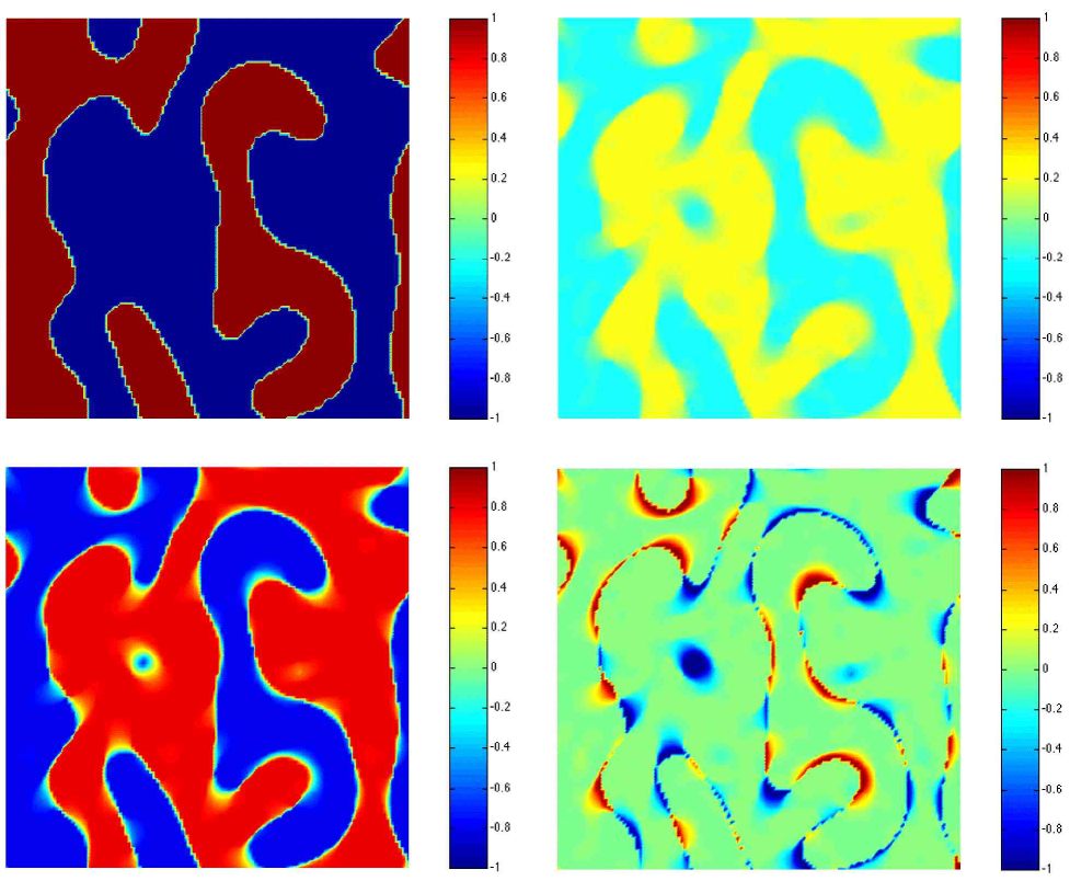
FIG. 1.: The present day values of $\Delta\Omega_{\Lambda}$ (top left), $\Delta\Omega_{m}$ (top right) and $-2\Delta h/h$ (bottom left), together with their sum (bottom right) for a particular numerical simulation in units of $|\Delta\Omega_{\Lambda}^{0}|$. The horizon size is about $1/4$ of the box size.

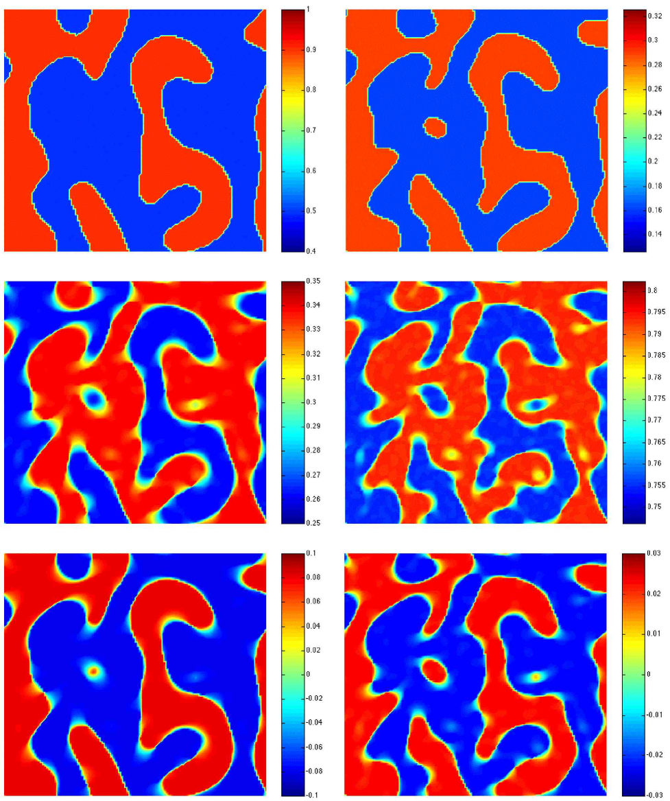
FIG. 2.: The values of $\Omega_{\Lambda}={\overline{\Omega}}_{\Lambda}+{\Delta\Omega}_{\Lambda}$ (top panels), $\Omega_{m}={\overline{\Omega}}_{m}+{\Delta\Omega}_{m}$ (middle panels) and $\Delta h/h$ (bottom panels) for a particular simulation box, for $z=0$ (left) and $z=1$ (right). Notice the different colour scales in the left and right panels. The horizon size at $z=0$ and $z=1$ is respectively about $1/4$ and $1/5$ of the box size.

- [1] J. Polchinski, String Theory, Cambridge University Press (1998).
- [2] E. W. Kolb & M. S. Turner, The Early Universe, Addison-Wesley (1994).
- [3] T. Banks, hep-th/9911067 (1999).
- [4] A. Chodos & S. Detweiler, Phys. Rev. D21, 2167 (1980).
- [5] W. J. Marciano, Phys. Rev. Lett. 52, 489 (1984).
- [6] Y. S. Wu & Z. W. Wang, Phys. Rev. Lett. 57, 1978 (1986).
- [7] E. Kiritsis, J.H.E.P. 10, 10 (1999).
- [8] S. H. S. Alexander, hep-th/9912037 (1999)
- [9] J. K. Webb et al., Phys. Rev. Lett. 82, 884 (1999).
- [10] C. Brans & R. H. Dicke, Phys. Rev. D124, 925 (1961).
- [11] S. Hannestad, Phys. Rev. D60, 023515 (1999).
- [12] M. Kaplinghat, R. J. Scherrer & M. S. Turner, Phys. Rev. D60, 023516 (1999).
- [13] L. Bergstrom, S. Iguri & H. Rubinstein, Phys. Rev. D60, 045005 (1999).
- [14] J. W. Moffat, Int. J. Mod. Phys. D2, 351 (1992).
- [15] J. W. Moffat, astro-ph/9811390 (1998).
- [16] J. D. Barrow & J. Magueijo, Phys. Lett. B443, 104 (1998).
- [17] A. Albrecht & J. Magueijo, Phys. Rev. D59, 043516 (1999)
- [18] J. D. Barrow, Phys. Rev. D59, 043515 (1999).
- [19] P. P. Avelino & C. J. A. P. Martins, Phys. Lett. B459, 468 (1999).
- [20] J. D. Barrow & J. Magueijo, astro-ph/9907354 (1999).
- [21] P. P. Avelino, C. J. A. P. Martins & G. Rocha, Phys. Lett. B483, 210 (2000).
- [22] P. P. Avelino & C. J. A. P. Martins, Phys. Rev. Lett. 85, 1370 (2000a).
- [23] J. D. Bekenstein, Phys. Rev. D25, 1527 (1982).
- [24] P. J. Peebles & B. Ratra, ApJ, 325, L17 (1988).
- [25] C. Wetterich, Nucl. Phys. B302, 668 (1988).
- [26] R. R. Caldwell, R. Dave, & P. J. Steinhardt, Phys. Rev. Lett. 80, 1582 (1998).
- [27] G. Huey G. et al., Phys. Rev. D59, 063005 (1999).
- [28] G. Starkman, M. Trodden & T. Vachaspati, Phys. Rev. Lett. 83, 1510 (1999).
- [29] P. P. Avelino, J. P. M. de Carvalho & C. J. A. P. Martins, Phys. RevLett. B501, 257 (2001). (2000).
- [30] S. Perlmutter et al., ApJ, 517, 465 (1999).
- [31] A. G. Riess et al., Astron. J., 116, 1009 (1998).
- [32] P. M. Garnavich et al., ApJ Lett., 493, L53 (1998).
- [33] A. Vilenkin & E. P. S. Shellard, Cosmic Strings and other Topological Defects, Cambridge University Press (1994).
- [34] W. H. Press, B. S. Ryden & D. N. Spergel, ApJ, 347, 590 (1989).
- [35] P. P. Avelino & C. J. A. P. Martins, Phys. Rev. D62, 103510 (2000).
- [36] S. Veeraraghavan & A. Stebbins, ApJ, 365, 37 (1990).
- [37] S. M. Carroll, W. H. Press & E. L. Turner, Annu. Rev. Astron. Astrophys. 30, 499 (1992).
- [38] D. J. Eisenstein, astro-ph/9709054 (1997).
- [39] P. P. Avelino & J. P. M. de Carvalho, M.N.R.A.S. 310, 1170 (1999)
- [40] A. K. Romer, P. T. P. Viana, A. R. Liddle & R. G. Mann, accepted for publication in ApJ, (astro-ph/9911499) (2000).
- [41] A. C. da Silva, D. Barbosa, A. R. Liddle & P. A. Thomas, astro-ph/9907224 (1999).
- [42] I. Zehavi & A. Dekel, Nature 401, 252 (1999).
- [43] R. Quast & P. Helbig, Astron. Astroph. 344, 721 (1999).
- [44] T. S. Kolatt &O. Lahav, astro-ph/0008041 (2000).
- [45] P. P. Avelino, J. P. M. de Carvalho & C. J. A. P. Martins, astro-ph/0103075 (to appear in Phys. Rev. D).
- [46] P. P. Avelino, A. Canavezes, J. P. M. de Carvalho & C. J. A. P. Martins, astro-ph/0106245.