Determining the reality of X-ray filaments

Abstract

A number of authors have reported filaments connecting bright structures in high-resolution X-ray images, and in some cases these have been taken as evidence for a physical connection between the structures, which might be thought to provide support for a model with non-cosmological redshifts. In this paper I point out two problems which are inherent in the interpretation of smoothed photon-limited data of this kind, and develop some simple techniques for the assessment of the reality of X-ray filaments, which can be applied to either simply smoothed or adaptively smoothed data. To illustrate the usefulness of these techniques, I apply them to archival ROSAT observations of galaxies and quasars previously analysed by others. I show that several reported filamentary structures connecting X-ray sources are not in fact significantly detected.

1 Introduction

With the advent of high-resolution X-ray telescopes it is now routine to see structure in X-ray images. Assessing the level at which one should believe this structure presents more of a challenge in X-ray observations than in optical or radio images of comparable resolution, because X-ray data are very often photon-noise limited. The problem is made worse by the common (and necessary) practice of smoothing the data with a Gaussian. This is carried out in order to make the images conform to our expectations of what the ‘true’ sky image with infinite exposure time would look like; but it is important to remember that in general it does not in fact take away the photon-limited nature of the underlying data.

A number of smoothed X-ray images of extragalactic objects appear, on published contour maps, to show quite clear ‘filamentary’ connections between X-ray sources in the field. (The term ‘filament’ does not have a single definition in the literature; I shall use it to mean any extended, apparently linear connection between two sources.) In this paper I discuss the techniques necessary to determine whether such filamentary connections are real, and apply them to some sample observations of galaxies and quasars, previously analysed by other authors (Arp 1996, Dahlem et al. 1996, Arp 1997), which I have taken from the ROSAT archives.

2 Significance and contouring

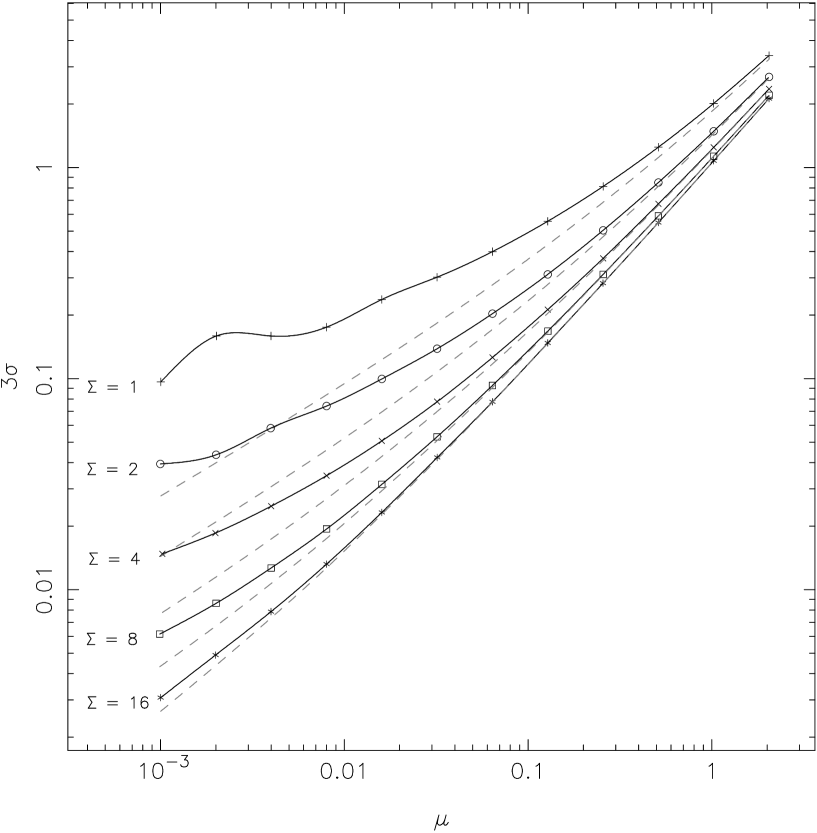
Figure 1: The true $3\sigma$ level derived from simulation as a function of the mean number of counts per pixel in the background ($\mu$) and the width $\Sigma$ of the convolving Gaussian (defined in the text; FWHM = $2.345\Sigma$). The solid lines are cubic splines fit through the data points derived from simulation. Deviations from a smooth curve seen for low $\mu$ and $\Sigma$ are a result of the Poisson-limited nature of the data. At high $\mu$, it will be seen that the $3\sigma$ level converges on a value close to $\mu$, as expected. At low $\mu$ and $\Sigma$, the difference between the $3\sigma$ level and $\mu$ is highly significant. The dashed lines below each solid line show the ‘mean plus three times r.m.s.’ contour levels derived from the same simulations. While they join the true $3\sigma$ lines at high $\mu$ and $\Sigma$, this quantity is clearly a very poor, systematically low estimator of the true $3\sigma$ value at low $\mu$ and $\Sigma$.

The first problem in assessing the reality of features in smoothed X-ray maps is that of the significance levels to be chosen when contouring. If the mean background count density is $\mu$ counts per unit area and the convolving Gaussian has the form $f(r)\propto\exp(-r^{2}/2\Sigma^{2})$, then, as pointed out in Appendix A of Hardcastle et al. (1998), the background noise is not normally distributed unless $\mu\Sigma^{2}\gg 1$, a condition which does not typically apply in the sort of datasets being considered here. It is therefore incorrect, for example, to take the r.m.s. dispersion of the background noise after smoothing, multiply by three, add the mean and call the resulting contour level ‘$3\sigma$’ as though it were the corresponding confidence level for normally-distributed noise. In general it is not. Contours for noise which is not normally distributed should ideally have the same properties as those for normally distributed noise, so that the contour referred to as the ‘$3\sigma$’ contour, for example, should exclude all but 0.135% of the background. But in the case where $\mu\Sigma^{2}\la 1$, there is no analytic solution to the question ‘what is the contour level corresponding to the $n\sigma$ level for normally distributed noise, for some $n$?’. Instead, Hardcastle et al. (1998) outline a Monte Carlo procedure for determining the correct significance level. In this procedure, fields of simulated Poisson noise are convolved with a Gaussian and the ‘$n\sigma$’ level is derived directly from the distribution of the resulting noise. (Results of this process for some sample values of $\mu$ and $\Sigma$ are plotted in Fig. 1.) If, on the other hand, $\mu\Sigma^{2}\gg 1$, then the noise will be approximately normally distributed and a simple analysis, described in Hardcastle et al. (1998), shows that the $3\sigma$ contour should be at $\mu+3\sqrt{\mu/4\pi\Sigma^{2}}$ counts per unit area.

It is common for authors not to state the method by which the ‘$3\sigma$’ (or other) levels in published contour plots of smoothed X-ray images were derived; in some cases, even the size of the convolving Gaussian and/or the binning scheme is not given. This practice makes it very difficult to assess the reality of features in such plots, and it is recommended that in all cases where the noise is not, or might not be, normally distributed authors should explain what they mean by ‘$3\sigma$’. In what follows, wherever I refer to a $2\sigma$ or $3\sigma$ level calculated by me, it will imply that I have derived it from simulated Poisson noise as described above.

3 The effect of the PSF

However, even when the $3\sigma$ level is correctly defined, such that a contour at this level would exclude all but 0.135% of the Gaussian-smoothed background noise, it is unfortunately not necessarily the case that we can say that all ‘structure’ around a bright source enclosed by such a contour is detected at a corresponding significance level. The radially averaged point-spread function (PSF) of X-ray instruments often has a very broad tail, so that there are expected to be significant count densities at large distances from the centroid; the shape of the PSF can be energy-dependent, so that these off-centre counts are likely to have a peculiar spectrum compared to either the point source itself or the background. When two point sources are placed close to each other, the natural consequence of this feature of the PSF is that we get an enhancement of the count rate which is at its greatest directly between them. Smoothing the data with a Gaussian may well bring this feature up above the noise, giving the appearance of a filament connecting the sources.

Figure 2: Simulated ROSAT HRI observations of the Seyfert NGC 4151 and a neighbouring BL Lac object, binned in 10-arcsec pixels and smoothed with a $\Sigma=3$ pixel Gaussian. At low contour levels, a variety of apparent filamentary structures of the type shown can be seen connecting the sources in about one in five simulated observations. The actual observations of this object are discussed in section 4.6.

So to assess the reality of filaments observed at a given contour level in smoothed images we must ask what is the probability of seeing such filaments under the null hypothesis, which is that the two sources are in fact not connected by any real feature on the X-ray sky. In general this too must be done by Monte Carlo simulation. I have written code which generates a Poisson-distributed noise background and two or more simulated sources, convolved with a suitable PSF, which match those seen on the sky. The simulated data are then smoothed with a Gaussian, and then either automatically or by eye it is possible to see whether a ‘filament’ at a given contour level joins them (in practice, the code does this using a simple recursive flood-fill algorithm). By repeating this procedure many times, we can directly estimate the probability that an observed filament would be seen under the null hypothesis, and so characterise its statistical significance. Only connections which have a very small chance of being seen under the null hypothesis can be described as statistically significant. An example of the kinds of apparent filaments that can result from low choices of contour levels even under the null hypothesis is given in Fig. 2.

4 Data and simulations

Table 1: ROSAT observations obtained from the public archive. The ROR number is the ROSAT Observation Request; an ‘h’ as the second letter denotes HRI data, a ‘p’ indicates PSPC.

Object	ROR number	Livetime (s)
Mrk 474	rp600448	12381
NGC 4651/3C 275.1	rp600450	10147
	rh800719	25157
NGC 3067/3C 232	rp700468	5376
NGC 4319/Mrk 205	rh600441	12272
	rh600834	34991
NGC 3628	rp700010	13387∗
	rh700009	13484
NGC 4151	rh700023	9162

^∗ After master veto rate filtering; see the text.

Using the techniques discussed above, it is possible to re-examine objects discussed in the literature. The ROSAT data listed in Table 1 were obtained from the public archive. Data were analysed using the IRAF Post-Reduction Offline Software (PROS).

The radially averaged ROSAT PSPC PSF is well known (e.g. Hasinger et al. 1995) and so, using a suitably integrated version of an analytical approximation to the PSF, it is simple to simulate PSPC observations. One complication is that the PSF is both energy-dependent and dependent on the off-axis angle of the source. Dealing with the energy dependence of the PSF is not hard, but would involve generating an energy-weighted PSF for each source. For simplicity, I choose to use the PSF at a single energy, in most cases 1 keV (the energy at which ROSAT is most sensitive); this is a conservative choice, in the sense that the PSF is narrowest at approximately this energy. The off-axis angle dependence of the width of the PSF is incorporated, though not the distortions which appear at far-off-axis angles; no source considered here is significantly affected by them. The actual PSF observed in a given observation is also affected by the ROSAT aspect reconstruction problems, which can introduce various kinds of elongation, but since it is very hard to determine the extent to which this affects a given observation, I have not included it in the simulations.

The ROSAT HRI PRF is more strongly affected by the aspect reconstruction problems, but, for simplicity, in the two cases where it is used in this paper I have just used the standard parametrization of David et al. (1997).

4.1 Mrk 474

Mrk 474 is a $z=0.041$ Seyfert galaxy adjacent to a $z=1.94$ quasar (Arp 1996). The Seyfert is a very strong X-ray source, while the point X-ray source identified by Arp with the quasar, located 170 arcsec to the NW, is only weakly detected in the PSPC observations.

Arp (1996) analysed the 0.5-2.0 keV PSPC data, and saw a filament connecting the Seyfert and quasar. It is not clear what binning scheme and smoothing Gaussian was used to produce his figures 1 and 2, but I obtain very similar results by binning by a factor 7 (so that each pixel is 3.5 arcsec) and smoothing with a Gaussian of $\Sigma=4$ pixels (14 arcsec). The results are insensitive to the exact values of binning and smoothing used. The mean number of background counts in the image per 3.5-arcsec pixel, close to the central source and after excluding all visible background sources is 0.0135, which, using the techniques described in section 2, corresponds to $2$- and $3\sigma$ levels in the smoothed dataset of 0.032 and 0.044 counts pixel^-1 respectively. The image is contoured with these levels in Fig. 3. Comparing this figure with Arp’s figures 1 and 2, it can be seen that my $2\sigma$ level is more or less equivalent to his $4\sigma$ level, while my $3\sigma$ level is close to his $5\sigma$ level. As shown in Fig. 3, the connecting ‘filament’ is not represented except at the $2\sigma$ level when the confidence limits are calculated correctly. Moreover, when I simulated this situation (using 30 net counts for the quasar, as measured by Arp (1996), and 6700 net counts for the Seyfert galaxy), I found that we expect to see a connection between the two sources at the $2\sigma$ level 65% of the time, and even at the $3\sigma$ level 30% of the time, if the two sources are in fact just adjacent point sources, because of the increased count density close to Mrk 474. The detection of the filament in this source is thus certainly not statistically significant.

Figure 3: The ROSAT PSPC image of Markarian 474 smoothed and binned as described in the text, with contours at $0.0319,0.0435,0.07,0.09,0.12\dots 0.30$ counts pixel^-1. The lowest contours correspond to the $2$ and $3\sigma$ levels derived from simulation.

4.2 NGC 4651/3C 275.1

The nearby (Virgo cluster) galaxy NGC 4651 is adjacent to the radio-loud quasar 3C 275.1 ($z=0.557$). In this case the quasar is a reasonably strong X-ray source, while the galaxy shows some weaker extended emission. Hardcastle & Worrall (1999) found the PSPC emission from the quasar to be consistent with that of a point source, although the HRI observations of the source suggest some extension on small scales, consistent with emission from a cluster (Hardcastle & Worrall 1999, Crawford et al. 1999). NGC 4651 has an optical jet or tail; Arp (1996) views this as evidence for ejection, while Wehrle, Keel & Jones (1997) suggest that the optical colours are evidence for a tidal origin.

Binning and smoothing the 0.1-2.0 keV energy band with the same parameters as I used for Mrk 474, and with a measured mean background count level of 0.0534 counts pixel^-1, the elongation of NGC 4651 in the direction of 3C 275.1 is clearly visible. The $3\sigma$ contour after smoothing is at about 0.110 counts pixel^-1, and the elongation is seen at this level [corresponding to a level somewhere between the $4$ and $8\sigma$ contours in figure 7 of Arp (1996)]. Taking the quasar as containing about 200 counts in the 0.1-2.0 keV energy band, and the galaxy as containing 120, I used simulations to determine whether, if the galaxy were really a point source, the effect of the quasar’s proximity could cause the observed extension; as expected from the images and from the comparative weakness of the quasar, the probability of obtaining such a strong result by chance is negligible. We can safely conclude that the extension of NGC 4651 is likely to be real. However, there is no evidence for a compact jet-like structure in NGC 4651 in the HRI image.

4.3 NGC 3067/3C 232

The radio-loud quasar 3C 232 ($z=0.534$) is adjacent to the starburst galaxy NGC 3067. In this case, too, the effect of contamination by the quasar’s PSF is small and the elongation seen by Arp (1996) in the 0.7–2.0 keV X-ray emission of NGC 3067 appears real; simulation shows that this degree of extension in the smoothed image is too great to be produced by chance, particularly as it is not directed towards the quasar (which is what we would expect for an artefact of the sort discussed in section 3).

Arp (1996) also reports filaments in smoothed 0.1-2.0 keV images connecting 3C 232 to stellar objects to the north and northeast. Arp binned the data here in 5-arcsec pixels and smoothed with a small Gaussian of $\Sigma=3$ pixels. The background noise level per 5-arcsec pixel in this energy band is 0.068 counts; the corresponding $3\sigma$ level is 0.15 counts pixel^-1, whereas Arp’s lowest contour appears to have been at 0.11 counts pixel^-1, somewhat below the $2\sigma$ level. Simulation shows that we would not expect a filament even at this level connecting 3C 232 with the northern stellar object by chance under the null hypothesis, which suggests that there is some real emission in between 3C 232 and the northern stellar object, but the data provide no significant evidence for such a filament rather than, for example, an intervening point source.

4.4 NGC 4319/Mrk 205

Arp (1996) observed the X-ray bright $z=0.07$ Seyfert galaxy Mrk 205 with the ROSAT HRI. The Seyfert lies 44 arcsec south of the galaxy NGC 4319, which was not detected in the HRI observations; but a number of other sources are detected in the field, including the early-type galaxy NGC 4291, 6.4 arcmin away to the NE, which is extended in the X-ray. Three of the brightest of these sources, at off-axis distances from 8 to 15 arcmin, are identified with intermediate-to-high redshift quasars. In addition to Arp’s data, a deeper exposure centred on NGC 4291 exists in the archive; this shows similar detections. Having adaptively smoothed his dataset (this process involves smoothing the pixels containing small numbers of photons with larger Gaussians than those containing larger numbers, and then summing the results) Arp obtained the ‘startling’ result that many — indeed, almost all — of the point sources were joined to the central source, Mrk 205, by ‘filaments’ of X-ray emission.

I began to investigate this field by analysing the data in a similar way to the other sources. Adopting Arp’s binning scheme of 8-arcsec pixels, the mean number of background counts per pixel $\mu$ is then about 1.08. I smoothed the whole image with a Gaussian of 16 pixel FWHM, or $\Sigma=6.80$ pixels; the corresponding $3\sigma$ level is 1.21 counts pixel^-1. (This result was derived from numerical simulation, but since $\Sigma^{2}\mu\gg 1$ in this case, the background noise is close to being normally distributed, and the analytic approximation described in section 2 in fact applies and gives the same answer.) At this level, or even at the corresponding $2\sigma$ level, no filaments connected any of the sources. Only at the $1\sigma$ contour level did the filamentary structure seen in Arp’s figure 10 begin to become apparent.

However, Arp’s use of adaptive smoothing is intended to improve the visibility of low-surface-brightness features. The characteristics of Poisson noise smoothed in this way are even less clear than for the single-Gaussian case, but the question may still be answered by Monte Carlo simulation as discussed in section 2. Arp’s description of his binning scheme is somewhat ambiguous, but I obtained a reasonable match to the image in his figure 10 by smoothing the 8-arcsec pixels containing one count with a Gaussian of $\Sigma$ (not FWHM) of 16 pixels, pixels with two counts with a Gaussian of $\Sigma=16/\sqrt{2}$ pixels, and so on ($\Sigma=16\times 2^{-(n-1)/2}$ pixels, where $n$ is the number of counts) up to pixels with more than 12 counts, which were not smoothed.

I then simulated the effects of smoothing Poisson-distributed noise with $\mu=1.08$ counts pixel^-1 with this adaptive filter. The resulting $3\sigma$-equivalent level (1.29 counts pixel^-1) is, as expected, higher for this smoothing method than for the case where the whole field is smoothed with the largest Gaussian (on the analytic approximation, this would be 1.13 counts pixel^-1), both because the ‘average’ smoothing Gaussian is smaller and because the method accentuates the difference between bright and faint noise pixels. As shown in Fig. 4, when contoured at this level my adaptively smoothed image shows no significant filaments; a much lower level of contouring is required to show up the structures in Arp’s figure 10. In fact, it appears from the caption from Arp’s figure 11a that his ‘$3\sigma$’ level is 1.08 counts pixel^-1, which is similar to the expected number of counts per pixel (unchanged, of course, as a result of smoothing). It is therefore not at all surprising that contouring at this level shows connections between adjacent sources; since the median for these data is close to the mean, this contour level corresponds to contouring about half the area of the map (preferentially the central regions, because of the effects of vignetting on the external component of the X-ray background). Simulating adaptive smoothing of the HRI field of view, neglecting vignetting, I find that we expect to see a connection at this level between the central source and the northernmost point source (identified with a $z=0.464$ quasar) approximately 25% of the time under the null hypothesis; the filaments in Arp (1996) are therefore not statistically significant. They are similarly undetected on the deeper HRI image centred on NGC 4291 (where the $3\sigma$ level of the adaptively smoothed image is lower as a fraction of $\mu$ because of the higher number of background counts per pixel).

Figure 4: The ROSAT HRI Markarian 205 field adaptively smoothed as described in the text. The lowest contour, 1.05 counts pixel^-1, shows up non-significant structure comparable to that in the image of Arp (1996). The next contour, 1.29 counts pixel^-1, is the $3\sigma$ level derived from simulation. This image shows the whole HRI field of view, which is approximately square with the vertices lying on the axes of the plot to the N, S, E and W of Mrk 205. (Note that some detected but faint point sources are not enclosed by the $3\sigma$ contour; this is because adaptive smoothing is optimized to emphasize low-surface-brightness extended emission, and tends to smear out the counts from weak point sources.)

4.5 NGC 3628

The starburst galaxy NGC 3628 was observed by Dahlem et al. (1996) and shows a striking filamentary structure, extending south from the galactic nucleus to a point source 2.7 arcmin away, in images in the 0.75 keV band (0.44–1.21 keV) and 1.5 keV band (0.73–2.04 keV); this point source itself appears connected to another point source a short distance to the SE, which Flesch & Arp (1999) identify with a $z=2.15$ quasar.

The contour levels selected by Dahlem et al. correspond quite well to the $3\sigma$ levels derived from simulation; after master veto rate filtering to match theirs and binning in 15-arcsec pixels I find a background count rate away from NGC 3628 in the 0.75-keV band of 0.23 counts pixel^-1, corresponding to a $3\sigma$ level of 0.73 counts pixel^-1, which is actually below their adopted $2.5\sigma$ level. The filament is thus apparent in contours at better than the $3\sigma$ level. Simulation (using a PSF appropriate for an energy of 0.75 keV) shows that the connection between the two adjacent point sources is not significant, but that a connection at the observed level between NGC 3628 and the source to the S is not expected to occur by chance. However, this does not take account of the extended X-ray halo found by Dahlem et al. (1996) around NGC 3628 (and clearly visible as excess emission in their figure 2). If we model this crudely as an extra uniform contribution to the background — taking the average in a region between NGC 3628 and the southern source, the background is pushed up to $0.59\pm 0.04$ counts pixel^-1 — then the connection between NGC 3628 and the point source can occur by chance in a few per cent of cases, so the feature is only marginally significant. Again, the filamentary emission is not seen in the HRI image, which supports the notion that we are seeing a region of extended emission rather than a true X-ray jet; but it will clearly be of great interest to obtain more sensitive images of this field. At the time of writing, a scheduled short Chandra observation has not yet been processed.

4.6 NGC 4151

Arp (1997) suggests that a filament connects this well-studied Seyfert galaxy to a $z=0.615$ BL Lac object 5 arcmin to the N in a ROSAT HRI image. Arp binned the HRI data into 10-arcsec (20-pixel) square bins; the off-source background is then 1.21 counts pixel^-1. It is not clear what Arp means when he says that he smoothed the data with a ‘$5\sigma$ Gaussian’; a $\Sigma=5$ arcsec Gaussian is very small given this binning scheme while a $\Sigma=5$ pixel Gaussian is very large, causing the two sources to overlap. I obtain images quite similar to those of Arp (1997) if I smooth with a $\Sigma=3$ pixel Gaussian (Fig. 5). The $3\sigma$ level derived from simulation is then 1.53 counts pixel^-1 (since $\mu\Sigma^{2}\approx 10$, the analytic approximation of section 2 gives a very similar answer). As Fig. 5 shows, the sources are not connected at the $3\sigma$ level with this choice of smoothing. A connection between the sources does appear at a much lower significance level, 1.35 counts pixel^-1, which is about $1.5\sigma$. Simulation shows that a connection at this level can occur by chance 20% of the time under the null hypothesis (some examples of the connections seen in simulations are shown in Fig. 2, where the lowest contour is at 1.35 counts pixel^-1). The connection seen in Fig. 5 is therefore not significant.

Figure 5: The ROSAT HRI NGC 4151 field smoothed and binned as described in the text, with contours at $1.35,1.53,2,3,4\dots 10$ counts pixel^-1. The lowest contour shows up non-significant structure at the level of the features seen in figure 17 of Arp (1997). The next contour is the $3\sigma$ level derived from simulation. This image may be compared to the simulated images of Fig. 2.

5 Conclusions

Using Monte Carlo techniques to find the distribution of pixel values in smoothed noise fields and to assess the reality of connections between adjacent sources, I have found that the filamentary X-ray connections between low- and high-redshift Seyfert galaxies and quasars reported by Arp (1996) are not statistically significant. I have confirmed that the X-ray extension of two low-redshift galaxies located near high-redshift radio-loud quasars, reported in the same paper, is significant. The filament extending south from NGC 3628, discussed by Dahlem et al. (1996), was shown to be marginally significant. The connection between NGC 4151 and a BL Lac object reported by Arp (1997) is also apparently not statistically significant.

These results suggest that it is necessary to be cautious in the interpretation of smoothed X-ray images, and I urge authors to apply the techniques I have described to any situation where the detection or non-detection of faint extended X-ray emission has important scientific implications.

- (1) Arp H., 1996, A&A, 316, 57
- (2) Arp H., 1997, A&A, 319, 33
- (3) Arp H., 1998, Seeing red: redshifts, cosmology and academic science, Apeiron, Montreal
- (4) Crawford C.S., Lehmann I., Fabian A.C., Bremer M.N., Hasinger G., 1999, MNRAS, 308, 1159
- (5) Dahlem M., Heckman T.M., Fabbiano G., Lehnert M.D., Gilmore D., 1996, ApJ, 461, 724
- (6) David L.P., Harnden F.R., Kearns K.E., Zombeck M.V., Harris D.E., Prestwich A., Primini F.A., Silverman J.D., Snowden S.L., 1997, U.S. ROSAT Science Data Center report, available at URL: http://hea-www.harvard.edu/rosat/rsdc_www/hricalrep.html
- (7) Flesch E., Arp H., 1999, A&A, submitted, astro-ph/9907219
- (8) Hasinger G., Boese G., Predehl P., Turner T.J., Yusaf R., George I.M., Rohrbach G., 1995, MPE/OGIP Calibration Memo CAL/ROS/93-015, version 1995 May 08
- (9) Hardcastle M.J., Worrall D.M., Birkinshaw M., 1998, MNRAS, 296, 1098
- (10) Hardcastle M.J., Worrall D.M., 1999, MNRAS, 309, 696
- (11) Wehrle A.E., Keel W.C., Jones D.L., 1997, AJ, 114, 115