Central cusp due to a super-massive black hole in axisymmetric models of elliptical galaxies

Abstract

We use numerical simulations to investigate the cusp at the centre of elliptical galaxies, due to the slow growth of a super-massive black hole. We study this problem for axisymmetric models of galaxies, with or without rotation. The numerical simulations are based on the ‘Perturbation Particles’ method, and use GRAPEs to compute the force due to the cusp. We study how the density cusp is affected by the initial flattening of the model, as well as the role played by initial rotation. The logarithmic slope of the density cusp is found to be very much insensitive to flattening; as a consequence, we deduce that tangential velocity anisotropy– which supports the flattening– is also of little influence on the final cusp. We investigate via two different kinds of rotating models the efficiency with which a rotation velocity component builds within the cusp. A cusp in rotation develops only for models where a net rotation component is initially present at high energy levels. The eventual observation of a central rotational velocity peak in E galaxies has therefore some implications for the galaxy dynamical history.

1 Introduction

HST observations have shown that a central density cusp is present in most, if not all, elliptical galaxies (Lauer et al. 1995, and companion papers). Furthermore the slope of the density cusp has shown a dichotomy between high mass (luminosity) systems and low mass (luminosity) ones, analogous to what has been found for other observational properties (Bender et al. 1989). Low mass ellipticals tend to host steep cusps, the radial profile of their luminosity $\rho(r)$ having a logarithmic slope $\gamma\equiv-{\rm d}log(\rho)/{\rm d}log(r)\simeq 1.9\pm 0.5$. On the other hand, luminous ellipticals have shallower cusps, with $\gamma\simeq 0.8\pm 0.5$ (Gebhard et al. 1996).

The most popular explanation for the formation of a density cusp is a central super-massive black hole (BH)– see Richstone et al. (1998), Kormendy & Richstone (1995) for reviews. Such BHs are believed to be present in a large fraction (possibly close to 1, Haenelt & Rees 1993, Tremaine 1997) of present day galaxies. Their influence on a collisionless galactic nucleus was first addressed by Peebles (1972), Young (1980), Goodman & Binney (1984) using semi-analytic models.

All these models suppose an isolated galaxy, at the center of which a BH grows by gas accretion. The slope of the cusp produced in such models is within the range observed for the less massive E galaxies. In this paper we shall also consider the formation of a cusp in an isolated galaxy, as we are interested in the origin for the steep cusp ($\gamma\simeq 1.9$) of low luminosity ellipticals. On the other hand, numerical simulations (Makino & Ebisuzaki, 1996, Quinlan & Hernquist 1997, Nakano & Makino 1999) have shown that a BH sinking within the core of an elliptical galaxy, or a binary of BHs produce a shallow cusp, similar to that observed for massive E galaxies. Such a BH binary could result from a merger. This picture is therefore compatible with the general belief (e.g. Nieto & Bender 1989) that the apparent existence of two classes of ellipticals is related to a more important role played by merging and interactions in the history of massive E galaxies.

All the semi-analytic models of cusp formation due to a central BH use the adiabatic invariance of actions to derive the distribution function after a BH has slowly grown (see Young 1980). Since actions are explicitly known for spherical systems, analytical models have been derived in spherical symmetry. Based on such quasi-analytic computations for spherical models, Quinlan et al. (1995) investigated the consequences of the initial density profile on the slope of the cusp, and addressed the influence of a velocity anisotropy.

For non-spherical systems – except for Stäckel potentials – an expression for the actions is unknown, and therefore models based on the conservation of actions have not been computed hitherto. In this paper, we propose to use numerical simulations with high central resolution, based on the PP method (Leeuwin et al. 1993), to investigate the cusp formed in axisymmetric systems by the growth of a BH.

Many low luminosity galaxies display little evidence for triaxiality, but are close to axisymmetry; they can be modeled as two-integral models, with $f(E,L_{z})$. Such a distribution function (d.f.) implies velocity dispersions obeying $\sigma_{R}=\sigma_{z}$, meaning that flattening would be due to an excess of azimuthal motion (which increases the net rotation, or the tangential anisotropy). This does not preclude that three-integral models would not do as well, or better (e.g. review by Merritt, 1998). Many of those galaxies however exhibit kinematic features consistent with isotropic rotators models: at least for them, an excess of tangential motion is plausibly the main support for their flattening.

The BH itself may have perturbed orbits sufficiently to erase the part of memory for initial conditions that corresponds to conservation of a third integral (Norman et al. 1985, Gerhard & Binney 1985, Merritt & Quinlan 1998). In this case axisymmetry is a consequence of the BH growth. Nevertheless, one still ought to investigate the scenario in which, for some of these galaxies, the presently observed axisymmetry already existed before the BH growth.

This is the goal of this paper, where we will study the cusp generated by the growth of a central BH within axisymmetric systems having various degrees of rotation. If a BH grows in a roughly axisymmetric galaxy, do the initial flattening and rotation have a sizeable effect on the evolution, so that it deviates from that of the well known spherical case? Could we in certain cases be able, eventually with more detailed observational data, to infer from the properties of presently observed cusps any information about the pre-black hole galaxy? Should one be cautious in certain cases about deriving the BH mass using the spherical adiabatic model?

This paper is organized as follows: first, the existing models are briefly recalled in section 2. We then specify the initial conditions (section 3) and the numerical techniques used for this work (section 4). Results for non-rotating and rotating models are given in sections 5 and 6, respectively. We conclude in section 7.

2 Previous models for galactic cusps

Previous models are based on a few basic assumptions, and ours will follow suit. The growth of the BH is supposed to be due to gas accretion, and thus does not deplete the original stellar component. The existence of the gaseous component is otherwise neglected, so that the models follow the evolution of a purely stellar component. The growth time $t_{BH}$ of the black hole is taken to be at maximum $\sim 10^{7}$ Yrs. This is long enough with respect to the stellar dynamical times, so that we can compare our models with the adiabatic computations, but not too long for obvious computation time reasons. It is furthermore reasonnable if compared to the ‘Salpeter time’, or timescale for the mass accretion onto a black hole:

$$t_{S}=M_{BH}/\dot{M}_{BH}\simeq\epsilon\times 4\times 10^{8}Yrs.$$ (1)

In the above, $\epsilon$ is the radiative efficiency, which is most often $\epsilon\leq 0.1$ in current models of accretion disks (cf. Richstone et al. 1998), or in estimates derived from quasars number counts (van der Marel 1997).

Furthermore the models neglect collisions. It has been estimated in the past that only some of the spiral galaxies bulges are dense enough to experience significant two-body interactions (see e.g. Kormendy 1988), although these estimates were based on the belief that elliptical galaxies had cores. Let us suppose for instance that up to $\sim 0.1-1\%$ of an E galaxy mass, corresponding to say $N\sim 10^{6}-10^{9}$ stars, is enclosed in the central $\sim 10$ pc, where velocity is of order a few times $\sim 100$ km/s. The crossing time in these regions should be $T_{cr}\simeq 10^{5}\;\left(\frac{R({\rm pc})}{10}\right)\;\left(\frac{100}{\sigma({\rm km/s})}\right)$ Yrs. Therefore the relaxation time would be (e.g. Binney & Tremaine 1987): $t_{rel}\simeq N/(8{\rm ln}N)\,t_{cr}\simeq 10^{9}\;\left(\frac{R({\rm pc})}{10}\right)\;\left(\frac{100}{\sigma({\rm km/s})}\right)\;\left(\frac{N}{10^{6}}\right)$ Yrs. Stellar collisions are liable to play some role over the age of the universe in such a system with an already highly concentrated density. For the models we consider here, however, a collisionless model is justified, given that the initial galaxy has a large core, and that the BH grows in $\sim 10^{7}$ Yrs. Nevertheless it should be kept in mind that collisional processes could play a role in the evolution of the center-most part after the cusp has developed.

The spatial extent of the cusp is given approximately by the influence radius $r_{I}$ of the BH, which is the distance up to which the BH potential dominates. This is estimated as:

$$\frac{M_{BH}}{r_{I}}\simeq\sigma^{2}_{0},$$ (2)

where $\sigma_{0}$ is the central velocity dispersion, and $M_{BH}$ is the BH mass.

2.1 Analytical models: spherical adiabatic models

Analytical models assume that the central BH grows over time scales that are long compared to dynamical times in the central region. The final d.f. can then be deduced from adiabatic conservation of actions (Peebles 1972, Young 1980).

In an isotropic system having initially a core, the cusp is predicted to have a slope $\gamma=3/2$ (Young 1980; see also Tremaine 1997). This value, however, holds if the BH mass is less than roughly the core mass; when larger, the self-gravity of the cusp becomes important and the slope increases up to values $\simeq 2$ (e.g. Young 1980). For centres that are initially ‘non-analytical’ – i.e. whose density profile has a non-zero derivative at the origin– Quinlan et al. (1995) derive larger slopes $\gamma$, with higher values for stronger initial cusps.

Goodman & Binney (1984) provide the following simple picture for the way orbits are transformed as the cusp grows. The fact that radial action is conserved plays an especially important role in the shape evolution of elongated orbits. It means that the radial excursion $r_{max}-r_{min}$ does not change much, but the potential center, which is originally at the orbit center (roughly harmonic potential), is finally at one of its foci (keplerian potential). Thus for elongated orbits eccentricity has decreased, which means also that the motion is more circularly biased. The adiabatic analytical models already cited predict indeed a moderate tangential anisotropy. This trend for rounder orbits is also present in numerical results by Norman et al. (1985), who studied how the shape of orbits close to a growing point mass is modified.

Initial anisotropies in the stellar velocities appear to have a weaker influence than an initial cusp (Quinlan et al. 1995). Due, however, to the small number of available analytical anisotropic models, this problem could not be thoroughly examined. One of the few anisotropic cases for which the cusp slope has been semi-analytically evaluated is a spherical model fully made of circular orbits. From conservation of energy and angular momentum, the final logarithmic slope is found to be $\gamma=9/4$ (Quinlan et al. 1995 ), significantly higher than for the isotropic case ($\gamma=3/2$). Therefore we could expect that in a model with some intermediate degree of tangentially biased motion, $3/2<\gamma<9/4$. Since our axisymmetric models are flattened in their centre by an excess of tangential motion, it is interesting to ask whether such an anisotropy will have a sizeable influence on the cusp slope. We may also ask whether a systematic rotation will bring any changes. These are some of the questions we will try to answer in this paper.

For the very few galaxies which had been observed ten years ago with sufficient central resolution, observations showed rotation velocities rising towards the center. This prompted attempts to compute the amount of angular momentum brought to the center by the forming cusp (Lee & Goodman 1989, hereafter LG89 ; see also Cipollina & Bertin 1994, hereafter CB94). These works, however, had to assume a spherical potential in order to derive analytical solutions. One aim of this paper is to address this problem anew without any such approximation. In sections 5 & 6, we investigate the influence of initial rotation for self-consistent axisymmetric models. Our motivations do not follow those of LG89, because higher quality, more recent observations no longer show evidence for more rotation than dispersion in the centre (see e.g. van der Marel et al. 1997, Joseph et al. 2000 for HST observations of M32, and Kormendy et al. 1998, regarding NGC 3377).

2.2 Numerical methods

The pioneering simulation by Norman et al. (1985) did not search for any detailed feature in the center, but was meant instead to measure the shape changes caused at moderate and large radii by a central growing BH. Due to the limited numerical capacity available at the time, their results displayed substantial particle noise, but showed already the trend towards axisymmetrization. Merritt & Quinlan (1998) recompute this problem with a considerably improved accuracy, obtained by using a larger number of particles ($N\sim 1.1\times 10^{5}$ instead of $N=2\times 10^{4}$ for Norman et al. 1985), and by enhancing the central particle density. To this end, they replace each strongly bound particle by a number of less massive particles distributed over its orbit (see §4.4).

Sigurdsson et al. (1995) built a numerical code to follow the growth of the cusp itself, and tested it for the spherical case. Their code makes use of the self-consistent field method (Hernquist & Ostriker 1992). This is formulated as a perturbation method, in the sense that it uses a family of density-potential functions, of which the zero-order term corresponds, or is close, to the initial model. At each time step during the simulation, the coefficients of the expansion for the density yield the new potential. The less the system evolves, the fewer are the terms required in the expansion to provide a given level of accuracy. In the implementation by Sigurdsson et al. (1995), the number of particles in the central parts is enhanced by using a mass spectrum for the particles. This is achieved by considering for the particles distribution, instead of the initial d.f. $f_{0}(E)$, a distribution $f_{0}(E)/m(E,L)$, such that the mass $m$ of a particle is less than unity if the pericenter of its orbit is smaller than some radius, and is unity if it is larger. This way, orbits reaching close to the centre are represented by more numerous, lighter particles. A numerical simulation based on this code, and using $512,000$ particles, has been performed by van der Marel et al. (1997), in order to check the stability of their dynamical model for M32, i.e. an axisymmetric model including a central supermassive BH.

In the present paper, we use a numerical perturbation technique which allows to concentrate particles at the center of the model, without entailing at the same time high particle-noise for the potential at larger radii (§4). In addition, we perform a subdivision of the central particles when necessary, to further increase the resolution at the center. These numerical simulations are used here in order to extend the models of BH induced cusps to non-spherical systems.

3 The initial axisymmetric model

3.1 Axisymmetric, non-rotating model

Fully analytical axisymmetric models for elliptical galaxies are scarce (Lynden-Bell 1962, Dejonghe 1986, Evans 1994, cf. discussion in Hunter & Qian 1993). Most of them are sums –often infinite sums – of Fricke terms. We take here the simple model by Lynden-Bell (1962), which uses only two Fricke terms:

$$f_{0}(E,L_{z})= F_{1}E^{7/2}+F_{2}L_{z}^{2}E^{13/2} ~{}~{}{\rm if}E>0$$ (3)

$$~{}= 0~{}~{}~{}~{}~{}~{}~{}~{}~{}~{}~{}~{}~{}~{}~{}~{}~{}~{}~{}~{}~{}~{}~{} ~{}~{}{\rm otherwise}$$

where $E$ is the binding energy $E=\Phi_{0}-v^{2}/2$ and $L_{z}$ is the component of angular momentum about the symmetry axis. This distribution corresponds to a flattened Plummer potential:

$$\Phi_{0}(R,z)=\frac{M_{0}}{((R^{2}+z^{2}+a_{P}^{2})^{2}-2b_{P}^{2}R^{2})^{1/4}},$$ (4)

where we have used cylindrical coordinates. In the above, $M_{0}$ is the total mass of the model, $a_{P}$ and $b_{P}$ are two parameters, and $F_{1}$ and $F_{2}$ are normalizing numerical constants, which expression is given by Lynden-Bell (1962):

$$\begin{array}[]{l l}F_{1}&=\frac{\sqrt{2}}{4\pi^{3/2}}\frac{5!}{7/2!}\frac{3a_{P}^{2}-2b_{P}^{2}}{M^{4}}\\ F_{2}&=\frac{\sqrt{2}}{4\pi^{3/2}}\frac{9!}{13/2!}\frac{5b_{P}^{2}(2a_{P}^{2}-b_{P}^{2})}{M^{8}}\\ \end{array}$$

We take in the following $a_{P}=4$ and $M_{0}=1$ in the units of the simulation. These are such that the mass unit is $10^{11}\,M_{\odot}$, the length unit is $1\,$ kpc, and $G=1$.

The core radius is usually defined as the radius at which the surface brightness $\Sigma(R,z)$ has decreased to half its central value $\Sigma_{0}$. This corresponds for the present model to $R_{1/2}\simeq 0.76~{}a_{P}$. The mass enclosed within the $\Sigma=cst$ isodensity level passing at $(R_{1/2},z=0)$ is $M_{core}\simeq 0.2~{}M_{0}$.

The flattening decreases with radius, so that the models tend towards spherical symmetry at large radii. The larger $b_{P}$, the larger the central flattening. $b_{p}$ however must be smaller than $b_{P~{}max}\simeq 0.64\,a_{p}$ otherwise the isodensity contours have a dimple on the z-axis. We shall consider a model close to the model with maximum flattening, by taking $b_{P}=0.55\,a_{P}$. For this model the axis ratio is about constant, with value $c/a\simeq 0.55$ (Fig. 1) within the region where the cusp will develop (see above the definition of the influence radius),

Since the d.f. depends only on $E$ and $L_{z}$, the velocity dispersions obey $\sigma_{R}=\sigma_{z}$. The flattening is sustained by an excess of motion in the $\phi$ direction, with respect to motion in the $R$ or $z$ directions. If velocity fields that are moderately biased towards tangential motion can affect the final density cusp, we should witness it in our computations.

The distribution function in Eq. 3.1 is even in $L_{z}$ and corresponds to a non-rotating system. In this case (cf. Lynden-Bell 1962):

$$\sigma_{R}^{2}= \frac{\Phi_{0}}{6}\left(1-0.2\frac{CR^{2}\Phi_{0}^{9}}{\rho_{0}}\right)\,=\,\sigma_{z}^{2}$$ (5)

$$\sigma_{\phi}^{2}= \frac{\phi_{0}}{6}\left(1+0.4\frac{CR^{2}\Phi_{0}^{9}}{\rho_{0}}\right) \hfil,$$ (6)

with $C=5b_{P}^{2}(2a_{P}^{2}-b_{P}^{2})/(4\,\pi M_{0}^{8})$.

                                 

Figure 1: Left panel: isodensity contours of the Lynden-Bell model with $a_{P}=4$ and $b_{P}=2.2$; the axis ratio for the density is shown as a function of the cylindrical radius in the insert. Right panel: velocity dispersion profiles $\sigma_{R}^{2}=\sigma_{z}^{2}$ and $\sigma_{\phi}^{2}$ along the $R$ axis for the same model

Fig. 1 displays the isocontours for the density, as well as the profile along $R$ for the velocity dispersions along each direction.

3.2 Rotating models

Models with positive net rotation are obtained by changing the sign of $L_{z}$ for a fraction of the orbits having negative $L_{z}$. If $\eta$ is the fraction of orbits being reversed, we obtain:

$$f^{r}(E,L_{z})=\left\{{f_{0}(E,L_{z})(1-\eta),\quad L_{z}<0}\atop{f_{0}(E,L_{z})(1+\eta),\quad L_{z}>0}\right.$$ (7)

In order however to avoid a discontinuity at $L_{z}=0$, the distribution function must have $f(E,L_{z})=f(E,-L_{z})$ for $L_{z}\rightarrow 0$. We therefore take for initial model:

$$f_{0}^{r}(E,L_{z})\equiv f_{0}(E,L_{z})\times(1+\eta p(L_{z})),$$ (8)

where $p(L_{z})$ is some function having value $\pm 1$, except for a small range around the origin, where it goes to zero. A simple choice is:

$$p(L_{z})=\left\{\begin{array}[]{l r}{\rm sin}\left(\frac{\pi}{2}\frac{L_{z}}{L_{m}}\right),&|L_{z}|<L_{m}\\ {\rm sign}(L_{z}),&{\rm otherwise}\end{array}\right.$$ (9)

Here $L_{m}$ is a parameter which determines the extent of the $L_{z}$ region where rotation is smaller than $\eta$. Its choice is of special interest for what follows.

The simplest choice for $L_{m}$ is a constant, independent of energy (cf. CB94). However, by taking some function $L_{m}(E)$, we can build models where, for any given energy, a constant fraction of orbits contribute to rotation. This is similar to the case studied by LG89. We investigate both types of models, as we know from comparing these two papers that they yield different results.

We thus consider two kinds of initial distributions, that use respectively:

$$p_{1}(L_{z})= p(L_{z}) \hskip-4.0pt{\rm with}\,L_{m}=L_{0}~{}~{}~{}~{}~{}~{}~{}~{}~{}~{}~{}$$ (10)

$$p_{2}(L_{z},E)= \hskip-4.0ptp(L_{z};E) \hskip-4.0pt{\rm with}\,L_{m}=xL_{c}(E),~{}0<x<1~{}$$ (11)

In the above definition, $L_{c}(E)$ is the angular momentum for the circular orbit with energy $E$, whereas $L_{0}$ is some constant, which is conveniently expressed in units of $l_{0}=a_{P}\sqrt{\Phi_{0}(0)}$.

The mean tangential velocity is given by:

$$v_{\phi}(R,z)=\frac{\int d^{3}v\,f_{0}^{r}(E,L_{z})(L_{z}/R)}{\int d^{3}v\,f_{0}^{r}(E,L_{z})}.$$ (12)

The effective rotation is measured by:

$$\eta_{e}=\frac{\int d^{3}r\,d^{3}v\,f(E,L_{z})L_{z}}{\int d^{3}r\,d^{3}v\,f(E,L_{Z})|Lz|},$$ (13)

which is in practice slightly smaller than $\eta$ in the definition of $f_{0}^{r}$ given by Eq. (8) (and exactly $\eta$ in the limit $L_{m}\rightarrow 0$).

4 Numerical method

A crucial feature for any $N$-body code aimed at studying the density cusp is of course the central resolution. Most particles should ideally orbit within a few times the ‘influence radius’ $r_{I}$ of the BH (Eq. 2). In this paper, we use a scheme which is formulated as a perturbation method, and allows to choose freely the sampling in phase-space. The main advantage of our scheme is that even if we have few particles outside $r_{I}$, where evolution is weak, the potential is fairly well represented (since it is dominated by the analytical $\Phi_{0}$ term, which has zero particle-noise).

4.1 The ‘perturbation particles’ scheme

The PP scheme has been described in detail elsewhere (Leeuwin et al. 1993). In this scheme, one writes the collisionless Boltzmann equation (CBE) as a perturbation problem. The unperturbed state corresponds to the initial analytical model, while the perturbation corresponds to the evolution of the system. Thus, the system d.f. is formally written as $f=f_{0}+f_{1}(t)$, where $f_{1}(t)$ is found by integrating explicitly the CBE along orbits in an N-body realization. The choice of the orbits to be integrated during the run –that is to say the initial distribution of particles $f_{S}({\bf r},{\bf v})$– is in principle arbitrary, but one should aim at a good sampling of phase-space regions where large perturbations are expected. The function $f_{S}$ is chosen to be a function of the system classical integrals (here $E,L_{z}$), so that in the absence of time evolution the sampling of phase-space is stationary.

If the system potential varies with time, $f_{S}$ can not be made a stationary function. However, both $f_{S}$ and $f$ obey the CBE equation. Therefore, noting the phase-space coordinate $w\equiv({\bf r},{\bf v})$, we may simply record the initial value $f_{S}(w(t_{0}))$ for each particle, since along each orbit $f_{S}(t)=f_{S}(t_{0})$. The mass attributed to the particle running on that orbit is weighted according to the local phase-space density:

$$m_{1}(t)=\frac{f_{1}(w(t))}{f_{S}(w(t_{0}))},$$ (14)

as explained in Leeuwin et al. (1993) and Wachlin et al. (1993).

On the other hand, the CBE is explicitly solved for $f_{1}$: the accuracy of orbits integration can then be monitored through the relative variations of $f$. The perturbation along an orbit is given by:

$$\frac{{\rm d}f_{1}(t)}{{\rm d}t}=-\left[f_{0},\Phi_{BH}+\Phi_{s.g.}\right]$$ (15)

where $\Phi_{BH}=M_{BH}/r$, and $\Phi_{s.g.}$ is the self- gravitating potential of the cusp.

The computation of moments for $f_{1}$ amounts in fact to a Monte-Carlo integral with sampling $f_{S}$. For instance, the perturbed total mass is evaluated as:

$$M_{1}\equiv\int f_{1}(w)~{}d^{6}w\simeq\Sigma_{i=1}^{N}\frac{f_{1}(w_{i})}{f_{S}(w_{i})}\simeq\Sigma_{i=1}^{N}m_{1i}.$$ (16)

To compute local values of the density field, or of any other field, the sum over the particles is of course limited to a small region of space where the quantity of interest is roughly constant. Moments of the total distribution $f=f_{0}+f_{1}$ are given by:

$$<V^{n}>=\frac{\int(f_{0}+f_{1})~{}V^{n}~{}d^{6}w}{\int(f_{0}+f_{1})~{}d^{6}w},$$ (17)

where $V$ represents any component of the velocity vector. This is estimated as:

$$<V^{n}>({\bf r}) = \frac{\int f_{0}~{}V^{n}~{}d^{6}w~{}+~{}\int f_{1}~{}V^{n}~{}d^{6}w}{\rho_{0}({\bf r})+\rho_{1}({\bf r})}$$ (18)

$$\simeq \frac{\rho_{0}~{}<V^{n}>_{0}~{}+~{}\Sigma_{i}\frac{f_{1}(w_{i})}{f_{S}(w_{i})}V^{n}_{i}}{\rho_{0}+\rho_{1}}$$

$$= \frac{\rho_{0}~{}<V^{n}>_{0}~{}+~{}\Sigma_{i}m_{1i}V^{n}_{i}}{\rho_{0}+\rho_{1}}$$

The sampling distribution $f_{S}$ is most efficient for the evaluation of the above Monte-Carlo integrals, when it is most similar to the integrants. The integration accuracy can be checked by monitoring the total mass in the perturbation, which should remain equal to zero. A convenient measure for the associated error is $M_{1}/||M_{1}||$, where we note $||M_{1}||\equiv\Sigma_{i}|m_{1i}|$.

The self-gravity of the cusp corresponds to the force due to the perturbation mass. Thus, a particle $j$ will be subject to a self-consistent force term:

$$\nabla\Phi_{s.g.}({\bf r}_{j})\simeq\Sigma_{i\neq j}\frac{m_{1i}}{|{\bf r}_{i}-{\bf r}_{j}|^{3}}({\bf r}_{i}-{\bf r}_{j}).$$ (19)

4.2 Orbit integration

Close to the BH, the force gradients are of course very large. Some orbits therefore demand extremely short time-steps during small time intervals. For such problems, adaptative time-steps is the most convenient scheme. In a 1D simulation (Leeuwin & Dejonghe 1998) that we ran to check whether the PP method could be advantageous for the present problem, we have experimented block time-steps integration (using either a leap-frog, or a RK4 scheme). In a block time-step scheme, the particles are sorted into groups at regular time intervals, and each group advanced with its smallest time-step until the next sorting out. This makes the scheme a costly one, since a set of particles may be advanced with a needlessly tiny timestep.

Symplectic methods (Wisdom & Holman 1991, Saha & Tremaine 1992), because they conserve phase-space volume, would in principle be useful to guarantee conservation of our sampling phase-space density (Binney, private communication). Unfortunately, symplectic integrators with adaptive time-steps do not yet exist (see Duncan, Levison & Lee 1998 for a version with block time-steps).

We use in this work the ODEINT routine due to Press et al. (1986), which is an adaptative individual time-steps scheme, based on a 4th-order Runge-Kutta time interpolation. The conservation of $f$ along orbits is better than $10^{-4}$ over each entire simulation.

4.3 Force computation with GRAPE machines

The BH mass was updated at each time-step. This is straightforward since the time dependence is explicit. Moreover, within the BH influence radius where the BH force term dominates, a precise evaluation is required.

The self-gravitating force (Eq. 19) is computed by direct summation of the individual particles contributions, using a GRAPE machine. A small modification of the standard software was necessary since the PP masses can be either positive or negative, a possibility not foreseen for GRAPE . Furthermore, timesteps within the cusp are very small, so that the cost of re-evaluating by direct summation the inter-particles force at each time-step for the most bound orbits would be prohibitive. Since the BH grows very slowly ($\sim 10^{7}$ Yrs) compared to the central dynamical times ($\sim 10^{5}$ Yrs, see §2.1), the force field due to the cusp also changes slowly with respect to individual crossing times. Moreover, it is negligible at large radii where dynamical times are larger (see Fig. 6). Therefore the self-consistent force field was evaluated using GRAPE only at regular time intervals $\Delta t$. To derive the self-gravity force experienced by each particle at intermediate times, we proceed as follows:

• The self-consistent forces are evaluated using  GRAPE   at regular time intervals $\Delta t$. This yields the three components $(F_{xi},F_{yi},F_{zi})$ of the force for each particle $i$. We infer for each particle the two components $(F_{Ri},F_{zi})$ along $R$ and $z$ in cylindrical coordinates.

• Using a cell-in-cloud (CIC, cf. Hockney & Eastwood 1981) scheme in polar coordinates, we compute the force field $(F_{R},F_{z})$ on a grid in $R,z$ (we average over the azimuthal angle $\phi$).

• At each time-step within $\Delta t$, the force $(F_{R},F_{z})(r_{i}(t))$ at the current position of each particle is interpolated from the grid values (with again a CIC).

The grid has $20\times 20$ cells, and extends in both directions from $x_{1}=r_{I}/200$ to $x_{20}=4\,a_{p}$. Points are spaced with a logarithmic increment:

$$x_{i+1}=x_{i}+dx_{i}\,k^{a},$$ (20)

where $a$ and $k$ are two real parameters numerically determined after the choice of $x_{1},dx_{1}$ and $x_{20}$. We have taken $dx_{1}=x_{1}$.

For the force evaluation with GRAPE we use a softening length $\epsilon=10^{-4}\,a_{P}$. The force is computed $1000$ times during the BH growth. At each time-step, the value for the self-gravity force is linearly interpolated from the grid values, using again a CIC scheme.

A run using $\simeq 3\times 10^{5}$ particles, and the parameters for the standard case defined hereafter (§5.1), takes approximately $2$ days on the Marseille 5 board GRAPE-3AF system, and somewhat longer on the GRAPE-4 system with 41 chips (see Athanassoula et al. 1998 for the characteristics of the Marseille GRAPE -3AF system, and Makino et al. 1997, Kawai et al. 1997 for the characteristics of the GRAPE -4 system). For $N=300,000$ particles, one force evaluation by GRAPE -3AF takes approximately $140$ s, therefore $\sim 38$h in the simulation are devoted to the computation of the self-gravity force field.

4.4 Choice of the sampling distribution

In order to ensure a stationary distribution (in the absence of any perturbation), $f_{s}$ must be a function of the isolating integrals of motion for the unperturbed potential $\Phi_{0}$. We are limited in the choice of analytical distribution functions $f_{s}(E,L_{z})$, as we were for $f_{0}(E,L_{z})$, because such models are scarce in the iterature. The known d.f.’s for axisymmetric systems are in general expressible as Fricke series, for which the self-consistent density can be calculated. The simplest choice is thus to consider a term from a Fricke series

$$f_{s}(E,L_{z})=F\,E^{\alpha}\,L_{z}^{\beta},$$ (21)

where $E=\Phi_{0}-\frac{v^{2}}{2}$ and $F$ is a normalizing constant. The corresponding density (see e.g. Dejonghe & de Zeeuw 1988) is given by:

$$\rho_{s}(R,z)=A\,F\,R^{\beta}\,\Phi_{0}^{\alpha+\beta/2+3/2},$$ (22)

with $A=\frac{\Gamma(\alpha+1)\Gamma(\beta/2+1/2)}{\Gamma(\alpha+\beta/2+1/2)}$. We can not generate a density of particles with a strong cusp using such a term. Models with a cusp in $R$ can in principle be built by choosing $-1<\beta<0$, however (i) their cusp in $R$ has a rather faint logarithmic slope $-1<\beta<0$; (ii) these are d.f.’s with a cusp in $L_{z}$, so their sampling of velocity space is very inhomogeneous. This is actually less unfavourable than it seems, since it favours nearly-radial orbits, which are actually those which experience the strongest perturbation (see §5.5). More freedom is available regarding the density decay at large radii. A steeper decline of density, with respect to the unperturbed model, follows from taking $\alpha>7/2+\beta/2$, as can be easily verified. We are not worried by the low corresponding particle density at large radii, since the potential there will be dominated by the analytical term.

Figure 2: Histogram for the normalized distribution of particles for each of the two sampling distributions $f_{S1}$ and $f_{S2}$ discussed in the text, as a function of the cylindrical radius $R$ (left) and of the spherical radius $r$ (right)

Here we experiment with two very different Fricke terms for $f_{s}$, in order to make sure that the choice of the sampling does not affect the measure of the cusp slope, which is our main objective. We use:

1. $f_{S1}$: $\beta=0,\,\alpha=8$.
   This is a model with a core, but its density falls much faster than the mass density of the unperturbed model. The central particle density is enhanced by splitting particles according to their energy and angular momentum, in a way similar to Merritt & Quinlan (1998). First particles are binned according to their binding energy $E_{0}$. For the most bound particles, we evaluate their pericenter $R_{min}(E,L_{z})$. If $R_{min}$ is smaller than the final BH influence radius (see §4.3), the orbit is selected for splitting. It is then integrated, within the unperturbed potential, for sufficient dynamical times. A number $n$ of phase-space positions along the orbit are recorded. Then the initial particle $(r(t_{0}),v(t_{0}))$ is replaced by $n$ particles, each of which is given one of the $n$ recorded positions and a statistical weight $\Gamma=1/[n\,f_{S}(r(t_{0}),v(t_{0}))]$. Usually, out of 20 equally sized bins in energy, we consider for splitting the $j=17\dots 20$ bins, take $n=(j-17)^{2}$, and repeat the whole procedure a second time (with $n=(j-15)$).

2. $f_{S2}$: $\beta=-0.9,\,\alpha=7$.
   This choice ensures a central density with cusp $\propto R^{-0.9}$, which proves an effective way to increase the central number of particles. We do not perform any splitting. On the other hand the sampling is very inhomogeneous in $R$ and $z$, as already mentioned.

The two particles distributions arising from the two sampling distributions just described are displayed on Fig. 2.

5 Cusps in non-rotating models

5.1 Cases considered

We assume a point mass is growing at the center of the model, by gas accretion, without depleting the stellar component (as in Young 1980, Quinlan et al. 1995, CB94, LG89). The BH mass grows over a time $t_{BH}$ from $M=0$ at $t=0$, to the final value $M_{BH}$ following (cf. Merritt & Quinlan 1998):

$$M(t)=M_{BH}\,\left(\frac{t}{t_{BH}}\right)^{2}\left(3-2\,\frac{t}{t_{BH}}\right).$$ (23)

For most of the runs discussed hereafter, we took $t_{BH}=10^{7}$ Yrs.

The potential due to the BH is modeled using a Plummer potential with smoothing length $\epsilon_{BH}$:

$$\Phi_{BH}=M/\sqrt{r^{2}+\epsilon_{BH}^{2}}.$$ (24)

We can choose $\epsilon_{BH}$ by imposing e.g.: $\epsilon_{BH}\ll r_{I}$. For instance, $\epsilon_{BH}\leq 10^{-3}r_{I}$. For the standard case, where $r_{I}\simeq 8\times 10^{-2}$, we have taken $\epsilon_{BH}=5\times 10^{-5}$, and verified that this value was small enough (§5.2).

We consider as the standard case one where the BH has a mass of $2\%$ the galaxy mass. This is supposed to be roughly representative of observational data. However, our flattened Plummer model does not have a realistic density profile, so that a more meaningful figure may be the ratio of the BH mass to the initial core mass. The latter is roughly $0.2\,M_{0}$ (see §3.1).

In addition, we discuss below experiments with higher BH masses, and different growth times. The summary of all the cases considered is to be found in Table 3. We will also consider, in the next section, models having initially some rotation. Those will be summarized in Table 4 of that section.

We display on Fig. 3 the results for the standard case. The sampling distribution used was $f_{S1}$. For that case, and other ones where the BH mass is very small, statistical noise is reduced by adding $10$ snapshots taken within a small time interval after $t_{BH}$. This is much less useful for the runs with larger BH masses (see below, Table 3). A polar grid has been used to produce the graphs, with $20$ points logarithmically spaced along $r$ (based on Eq. 20), and $10$ points equally spaced within $[0,\pi/2]$ along $\theta$, which is the angle from the $z$ axis. The smallest value $r_{1}$ of the $r$- grid is chosen so that the total snapshot has at least $1,000$ particles with $r<r_{1}$.

Quantities associated to the particles correspond to perturbed quantities. The related grid quantities ${\bf a}_{1,kl}$ at grid points $(r_{k},\theta_{l})$ are derived by applying a CIC scheme in the polar geometry. The total fields are finally recovered by adding the corresponding unperturbed analytical terms evaluated on the grid points. Thus for the total density:

$$\rho_{kl}=\rho_{0}(r_{k},\theta_{l})+\rho_{1,kl}.$$ (25)

Similarly the velocity components and dispersions are derived by adding the analytical terms, using Eq. 18, for $V=V_{R},V_{\phi},$ and $V_{z}$, and $n=1,2$. Fig. 3 shows isolevel contours for the total density at the end of the simulation, as well as for the total velocity dispersion $\sigma^{2}=\sigma_{R}^{2}+\sigma_{z}^{2}+\sigma_{\phi}^{2}$. The dash-dotted curves show the initial, unperturbed quantities. Also displayed (first row) are the curves $\rho_{k,1}$ and $\rho_{k,10}$, which give approximately the profiles of the total density along $R$ and $z$, respectively. The same is drawn on the bottom row for the square total dispersion $\sigma^{2}$. The dotted segments on these graphs indicate a line with logarithmic slope respectively $3/2$ for the density, and $1$ for the square total dispersion.

Therefore, the figure shows that even for the less massive BHs considered in this work, the central cusp is well resolved in two-dimensions. The maps also show that the central region has become very nearly spherical; the final axis-ratio is displayed on Fig. 4 as a function of the major-axis radius, scaled to $r_{I}$. By eye inspection of 3, the slope for the velocity is very similar to what is expected theoretically; also the density cusp appears to be similar to what is predicted for an initially spherical model. The cusp slopes will be measured with more care and discussed further in §5.4. We now turn to some runs performed in order to check our computations.

Table 1: Parameters for the ‘standard’ run

Final $M_{BH}/M_{0}$	$0.02$
Time for BH growth	$10^{7}$ Yrs
Smoothing length for the BH …	$5\times 10^{-5}a_{p}$
Number of particles	$\sim 300,000$

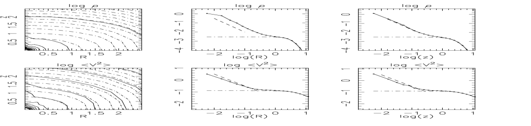
Figure 3: The two left panels show iso- contours for the density (top) and the total velocity dispersion (bottom), for the final model in the standard run (solid lines). The levels are logarithmically spaced. The initial model is shown by the dash-dotted lines (using different logarithmically spaced levels). The initial (dots) and final (full line) profiles along resp. the $R$ axis, and the $z$ axis, are also displayed, using logarithmic scales.

Figure 4: Minor to major axis ratio, as a function of $R$ scaled to the influence radius $r_{I}$, for the standard run (solid line). The dashed line shows the axis ratio for the initial model.

5.2 Numerical checks

A run was first made for $b_{P}=0$, in order to check that the slope obtained for a spherical potential agrees with the analytical estimates for this case. Its slope is measured, in the way we will explain in §5.4, both for the density and the velocity dispersion. We measure respectively $\gamma_{\rho}\simeq 1.52\pm 0.02$ for the density, in good agreement with the adiabatic model (and the simulation by Sigurdsson et al. 1995), and $\gamma_{\sigma^{2}}\simeq 0.94\pm 0.05$, very close to unity, as expected in the nearly Keplerian potential produced around the BH.

We also made some numerical checks for the standard axisymmetric run. First of all, the simulation was pursued after the BH growth time for an equal duration, in order to verify that a stationary model had been reached. The influence of the smoothing length $\epsilon_{BH}$ used in the BH potential was tested, by comparing runs using either a larger ($\epsilon_{BH}=10^{-4}\,a_{P}$) or a smaller ($\epsilon_{BH}=2\times 10^{-5}\,a_{P}$) smoothing length. The larger value produced a slightly shallower cusp, but results were unaffected for the smaller value. Therefore we use $\epsilon_{BH}=5\times 10^{-5}\,a_{P}$ in all subsequent runs –including those with larger BH masses, where a larger value of $\epsilon_{BH}$ could have sufficed.

We have experimented with both the $f_{S}$ described in §4.4. The final model obtained, for the parameters of the standard case, but using $f_{S2}$ instead of $f_{S1}$, is shown on Fig. 5. Results can be seen, by comparing to Fig. 3, to be extremely similar to those obtained when using the other sampling distribution, in spite of the fact that $f_{S1}$ and $f_{S2}$ are very different functions. The first sampling ($f_{S1}$) turned in practice to yield results with apparently somewhat less particle-noise for the density. This is probably due to the fact that $f_{S1}$ corresponds to a particle distribution which is similar along the $R$ and $z$ axes, while $f_{S2}$ has a cusp only in $R$. This may for instance explain why the spherically averaged cusp has more mass for $f_{S1}$ than for $f_{S2}$ (see Fig. 8). Some perturbation mass may be less well sampled in the $z$ direction. The differences, however, remain marginal. The two sampling functions give estimates for the logarithmic slope of the cusp (see 5.4) that can not be distinguished, within the error bars. Therefore we are confident that our results are not affected by the initial particle distribution.

A few runs were also performed in order to make sure that the results do not depend significantly on numerical parameters, such as the spacing of the grid used for the force evaluation (§4.3), the total number of force computations by GRAPE (§4.3), or the choice that we made for the number of particles $N=3\times 10^{5}$.

Figure 5: Same as the previous figure, also for the parameters of the standard case, but using $f_{S2}$ for the particles initialization, instead of $f_{S1}$. The layout is as for Fig. 3.

5.3 Importance of the cusp self-gravity

The perturbed central densities are high, but within small volumes. Therefore the mass in the cusp is not necessarily very large. Applying Eq. 2 to the Lynden-Bell model we find for the influence radius:

$$r_{I}\simeq 2\,a_{P}\frac{M_{BH}}{M_{0}}.$$ (26)

For the standard run $M_{BH}/M_{0}=0.02$, thence $r_{I}\simeq 0.16$. Initially, the mass enclosed in this radius is roughly (neglecting the effects of flattening): $M_{0}(r_{I})\simeq M_{0}(r_{I}/\sqrt{r_{I}^{2}+a_{P}^{2}})^{3}\simeq 2\times 10^{-5}M_{0}$. At the end of the simulation, we find it is: $M(r_{I})=M_{0}(r_{I})+M_{1}(r_{I})=M_{0}(r_{I})+\Sigma_{(r_{i}<r_{I})}\,m_{1i}\simeq 2\times 10^{-5}+6\times 10^{-4}\simeq 6\times 10^{-4}\,M_{0}$. Therefore the mass within the cusp remains a small fraction of the system mass.

On the other hand, the system has been affected by the central mass in a region much larger than the cusp itself. This can be seen from the radial distribution of the perturbation mass density, displayed on Fig. 6 for the standard case. For $r\geq 2$, $\frac{dM_{1}(r)}{dr}<0$, corresponding to orbits that have been requisitioned in order to build the cusp; this negative perturbation extends far from the center. As a consequence, the cumulated mass $M_{1}(r)$ decreases after $r\simeq 2$. It is $10\%$ of its maximum value at $r\simeq 5$. Outside this radius the cusp force is practically zero (Fig. 6). The orbital participation will be further described below (§5.5).

                                     

Figure 6: Left: The radial distribution of perturbation mass $dM_{1}/dr$ (solid line) and the cumulated distribution $M_{1}(r)$ (dashed line), for the standard case with $M_{BH}/M_{0}=0.02$, in percents of $M_{0}$. Right: Comparison between the forces due to the unperturbed mass distribution (dashed line), the BH (solid line), and the cusp gravity (dotted line). The insert shows the ratio of the cusp force $F_{1}$ to the total force $F_{0}+F_{1}+F_{BH}$, in percents.

We may estimate the self-consistent force (due to the cusp itself) $F_{s.g.}=\nabla\Phi_{1}$ within the influence radius, where we assume $\rho_{1}(R,z)\approx K\,r^{-3/2}$. A reasonable rough guess for $K$ is such that $\rho_{1}(r_{I})\approx\rho_{0}(r_{I})$. This yields a roughly correct ‘calibration’ for the central value, in agreement with the numerical value at the end of the simulation. Fig. 6 displays the different radial force terms: $F_{0}=\nabla_{R}\Phi_{0}$, $F_{1}=\nabla_{R}\Phi_{1}$, $F_{BH}$. Within a substantial fraction of the initial core radius ($\sim 0.75~{}a_{P}=3$), the unperturbed force is negligible. The BH dominates the central region, within roughly $a_{P}/4$, by a factor scaling from $10^{4}$ at $R\simeq 0$ to $10^{2}$ at $R\simeq r_{I}$. The self-consistent force contribution reaches at most $\sim 1\,\%$ for $M_{BH}/M_{0}=0.02$. Therefore we have neglected it for most runs with this BH mass. The self-gravity contributes at most for $\simeq 2\%$ when $M_{BH}/M_{0}=0.03$ (see Table 3). This is still very small, therefore we have also neglected the cusp self-gravity for models with $M_{BH}/M_{0}=0.03$.

The self-consistent term is not negligible, however, for the larger mass ratio $M_{BH}/M_{0}=0.2$ considered in this work, since it contributes for up to $\sim 15\%$ of the total force at $R\simeq a_{P}/4$ (Fig. 7).

                                    

Figure 7: Same as Fig. 6 but for a BH with mass $M_{BH}=0.2\,M_{0}$

5.4 Measure of the cusp slope

The Poisson noise due to the discretisation into particles varies with the number of particles as $1/\sqrt{N}$. To reduce it, we continue the simulation for another $0.5\times 10^{7}$ Yrs, and draw 10 snapshots, at regular time intervals. The snapshots are then merged, and this snapshot of $10\,N\simeq 3\times 10^{6}$ particles is analyzed. This is especially useful for the runs with $M_{BH}/M_{0}=0.02$, and, to a lesser extent, $M_{BH}/M_{0}=0.03$.

The central region (within $\sim~{}r_{I}$) is very nearly spherical, as can be seen from the 2D contour map of $\rho(R,z)$ (Fig. 3). Therefore, in order to measure the cusp slope, we can integrate over the $\theta$ angle of the polar coordinates $(r,\theta)$. A logarithmic grid in $r$ is built, using Eq. 20 and such that the sphere with radius the first grid point $r_{1}$ encloses $\simeq 1000$ particles. The spherically symmetrized density and velocity dispersions are evaluated at the grid points, and these grid values used to derive the corresponding logarithmic slopes.

Figure 8: Spherically symmetrized profiles for the density and velocity dispersions for the standard run. The total velocity dispersion (thick line) and the dispersions along each direction are displayed. The sampling distribution used is resp. $f_{S1}$ (top) and $f_{S2}$ (bottom). The positions of the filled squares indicate the grid used; the lines indicate slopes $\gamma=3/2$, for the density, and $\gamma=1$ for $\sigma^{2}$

The logarithmic slopes $\gamma_{\rho}$ for $\rho(r)$, and $\gamma_{\sigma}^{2}$ for $\sigma^{2}(r)$, are evaluated by computing the respective average logarithmic derivative over the grid points in some interval $I_{r}=[0,r_{max}]$. To estimate the error in this measure, we also compute the slope for each individual snapshot, and infer the mean deviation.

The radius $r_{max}$ should in theory be $r_{max}\approx r_{I}$. In practice, we take the maximum interval in which the radial profile appears as a straight line when plotted in logarithmic axes. This leads actually to consider a slightly smaller interval than $[0,r_{I}]$ for $\sigma^{2}(r)$, in order to avoid the transition region from cusp to core (see Fig. 8). Including grid points that belong to this transition region would obviously lead to a systematic under-estimate for the cusp slope.

This point is illustrated in Table 2, for the standard case with $M_{BH}/M_{0}=0.02$. This is the case where the measure depends the most on the choice of $I_{r}$. Indeed, the less massive the BH, the fewer the grid points contained within $r_{I}$. As a consequence, each of the grid points has a larger statistical weight in the average slope.

Of course, the value of the slope for $\sigma^{2}$ must be $1$ in the region where the BH dominates the dynamics. As can be seen from the table, the effects of excluding successively $r_{N}$, $r_{N-1}$ etc. from the $N$ grid points within $[0,r_{I}]$ are, for $\gamma_{\sigma^{2}}$: (i) to increase the average slope estimate (ii) to increase the mean deviation around the average value, as fewer data points are made available.

If we exclude the $2$ points lying within the cusp/core transition, the logarithmic slope measured for $\sigma^{2}$ is very nearly equal to unity, as it should be.

Table 2: The value of the logarithmic slope, estimated for respectively $\rho(r)$ and $\sigma^{2}(r)$; the mean deviation is also indicated. The case shown is for $M_{BH}/M_{0}=0.02$, and $f_{S}=f_{S1}$. The successive columns correspond to taking different fractions of the total number $N$ of grid points within $[0,r_{I}]$ –see text.

	$n=N=8$	$n=N-1$	$n=N-2$
	$(r_{max}=r_{I})$
$\gamma_{\rho}$	$1.46\pm 0.06$	$1.43\pm 0.05$	$1.43\pm 0.06$
$\gamma_{\sigma^{2}}$	$0.93\pm 0.05$	$0.99\pm 0.06$	$1.01\pm 0.08$

As for the density, there are up to 8 points that lie well within the cusp (Fig. 8). Our density profile deviates slightly from a pure power-law at the 2 inner points. Therefore we obtain a better estimate of the slope in the linear section by taking into account the full set of points within $r_{I}$. With these grid points, we find for the standard case:

• using $f_{S1}$ : $\gamma_{\rho}\simeq 1.46\pm 0.06$

Fig. 8 also displays the density and velocity profiles obtained when the sampling distribution is $f_{S2}$. The central density value is slightly smaller than with the previous case, probably because the sampling is not as efficient due to its strong spherical asymmetry. The value measured for the density logarithmic slope is now:

• using $f_{S2}$ : $\gamma_{\rho}\simeq 1.35\pm 0.15$,

This value is somewhat smaller than the value for the other sampling, but still consistent with it. We therefore conclude that the two sampling distributions tested, in spite of their different behaviour in the centre, yield similar results. We therefore believe the results are not an artifact of the method used. The value of $\gamma_{\rho}$ is consistent, within its error bars, with the value given in the literature for the spherical case, $\gamma=3/2$. We find no evidence for a significantly larger, nor smaller, slope.

Table 3: List of experiments with non-rotating models, with their numerical results. Column 4 gives the logarithmic slope measured for the density, and column 5 gives that for the total velocity dispersion. $||M_{1}||$ gives an estimate of the mass in the perturbation. $F_{max}$ is the maximum relative contribution to the total force of the self-gravity force. The last column gives an estimate of the relative error made in evaluating the perturbed quantities (see §4.1).

$\begin{array}[]{c}M_{BH}\\ \hline\cr M_{0}\end{array}$ $\begin{array}[]{c}M_{BH}\\ \hline\cr M_{core}\end{array}$ $\begin{array}[]{c}T_{grow}\\ {\rm(Yrs)}\end{array}$ $\gamma_{\rho}$ $\gamma_{\sigma^{2}}$ $||M_{1}||$ F_max $\begin{array}[]{c}M_{1}\\ \hline\cr||M_{1}||\end{array}$ 0.02 (spherical) 0.1 $10^{7}$ $1.52\pm 0.02$ $0.94\pm 0.05$ $0.05$ 0.01 $0.08$ 0.02 (standard) 0.1 $10^{7}$ $1.46\pm 0.06$ $1.01\pm 0.08$ $0.05$ 0.02 $0.05$ 0.03 0.15 $10^{7}$ $1.50\pm 0.04$ $0.98\pm 0.02$ $0.06$ $0.02$ 0.03 0.2 1 $10^{7}$ $1.71\pm 0.01$ $0.99\pm 0.01$ 0.4 0.15 $-0.02$ 0.03 0.15 $10^{6}$ $1.31\pm 0.1$ $0.92\pm 0.06$ $0.07$ $0.02$ $0.02$ 0.03 0.15 $10^{5}$ $0.92\pm 0.27$ $0.96\pm 0.08$ $0.07$ $0.02$ $0.02$

The results found for experiments using a larger final BH mass are discussed in §5.7. For such cases, the dispersion in the measures is very small (see Table 3), as the number of points useful for the measure is larger.

5.5 Orbital response to the BH

When we use the PP method, we have direct access to the distribution functions $f_{0},f_{1}$ and $f(E,L_{z})=f_{0}+f_{1}$. Those are available with a large signal-to-noise ratio, even for the case where the BH mass is only $1\%$ of the model mass, that we analyse in this paragraph.

The initial model can be viewed by plotting the surface $f_{0}(E_{0},L_{z})$, with $E_{0}=\Phi_{0}-{v^{2}}/{2}$ the unperturbed energy. Since $\Phi_{0}(r=0)=0.25$, $0<E_{0}<0.25$. This surface, drawn from a set of initial conditions for the particles, is shown on Fig. 9 (central panel). We use a regular grid in $E_{0}$ and $L_{z}$ to bin the particles, and sum the masses $m_{0i}=f_{0}(w_{i})/f_{S}(w_{i})$ within each cell of the grid. It could of course have been drawn analytically, but, as it is, the figure shows how smooth the numerical realization is. A map using a linear grey scale is shown on top of the surface. At fixed energy, the d.f. increases with increasing $L_{z}$, as can be seen from the figure. This is related to the excess of tangential motion supporting the flattening.

In a similar way, using snapshots at the end of the standard run, we can build the surfaces $f_{1}(E,L_{z})$ and $f(E,Lz)$. We plot in fact two slightly different maps. (i) A map of $f_{1}$ as a function of the initial values of $E_{0}$ and $L_{z}$ – $L_{z}$ is anyway conserved during the BH growth– reveals which orbits have been most perturbed. (ii) On the other hand, a map for $f(E,L_{z})=f_{0}(E,L_{z})+f_{1}(E,L_{z})$ (with $E=\Phi_{0}+\Phi_{BH}+\Phi_{s.g.}-\frac{v^{2}}{2}$ the total final energy) yields information about the orbital structure in the final model. In practise and for the sake of simplicity, we neglect the self-gravity of the cusp (we have shown in §5.3 that the self-gravity contribution is small for $M_{BH}/M_{0}\leq 0.03$), and plot $f(E^{*},L_{z})$, where $E^{*}\equiv\Phi_{0}+\Phi_{BH}-\frac{v^{2}}{2}$.

The map for $f_{1}$ is show on Fig. 9 (left panel). Positive values of $f_{1}$ are displayed in grey shades darker than the background (with white contour lines), whereas negative values appear as lighter shades (with black contour lines). The map shows that orbits having $E_{0}\simeq\Phi_{0}$ have been the most perturbed. Also, at a given energy, the perturbation is more important for orbits with small angular momentum $|L_{z}|$. For the most bound orbits ($E_{0}\simeq\Phi_{0}$), $f_{1}>0$, reflecting the fact that they now belong to phase-space regions more populated than initially. By contrast, a negative perturbation ($f_{1}<0$) can be found for smaller values of $E_{0}$, and $L_{z}\simeq 0$. These orbits have an apocenter located at a radius much larger than the influence radius. The fact that the perturbation extends much further than the influence radius was already seen in Fig. 6 (§5.3).

                                                                                           

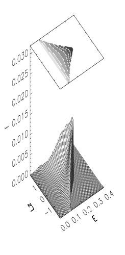
Figure 9: Distribution functions for the case without net rotation. The left panel shows the perturbation distribution $f_{1}(E_{0},L_{z})$ as a function of the initial unperturbed energy and angular momentum of the particles. The grey scale is dark for positive values, scaling linearly from $10^{-5}$ to $4\times 10^{-3}$ (with white contours over-imposed), and light (with black contours) for negative values. The 3-D plots display the initial $f_{0}(E_{0},L_{z})$ (center) and final $f(E,L_{z})$ (right) distribution functions– see text for details on the corresponding $E,L_{z}$ axes.

We have used 10 snapshots, issued at the end of the simulation and merged together, in order to produce the surface $f(E^{*},L_{z})$ shown on the right panel of Fig. 9. The final total distribution shows most clearly that only orbits with $L_{z}\simeq 0$ have a final energy $E^{*}>\Phi_{0}(r=0)$ (Fig. 9). These are orbits such that $\Phi_{BH}-\frac{v^{2}}{2}>0$, i.e. orbits that have become bound to the BH potential. Such orbits must provide an important contribution to the cusp. However, the fact that nearly radial orbits are more efficiently attracted into the cusp, does not imply radially biased motion within the cusp, since these orbits get rounder (see also CB94). In models with a central cusp, constructed either with, or without, a BH, Dehnen (1995) and Dehnen & Gerhard (1994) find that such orbits typically have $L_{z}\simeq L_{c}(E)$.

The final d.f. appears remarkably constant at high binding energies ($f(E)\simeq cst$ for $E>\Phi_{0}(0)$ and $Lz\simeq 0$). Tremaine et al. (1994) have built analytical models for spherical systems with a central density cusp and a central BH. For a cusp with slope $\gamma=3/2$, their d.f. tends to a constant for high binding energies, in a way very similar to our results.

The final d.f. can therefore be said ‘degenerate’ at high binding energies, in the sense that different energy levels have the same probability. Such a degeneracy is also typical of violently relaxed systems (see Lynden-Bell 1967, Chavanis & Sommeira 1998). Our results therefore support those by Stiavelli (1998), who has shown that the observable signatures of an adiabatically grown BH, on the one hand, and of violent relaxation around a pre-existing BH, on the other hand, are very similar. We have shown that this is due to the fact the distribution functions themselves have very similar behaviour at high energies.

5.6 Influence of growth time

The influence of the BH growth time on the final cusp has been checked, by experimenting with shorter times ($T_{BH}=10^{6}$, $10^{5}$ Yrs), for the case $M_{BH}/M_{0}=0.03$. The dynamical times within the cusp are close to $10^{5}$ Yrs, therefore the assumption of adiabaticity does not hold for the latter case. Moreover, some orbits may not have had time to rearrange into an equilibrium during the BH growth. Therefore all simulations are pursued after the BH has reached its final mass, so that the total time is $10^{7}$ Yrs for all cases.

Results for the logarithmic slopes are reported in Table 3. In good agreement with Sigurdsson et al. (1995), we found that the adiabatic model is still roughly valid for growth times of order $\sim 10\,T_{dyn}$. Nevertheless small growth times introduce some differences, and already for $T_{BH}=10^{6}$ Yrs, there is a tendency for the cusp to spread over a larger diameter. Whereas the density profile follows a power-law in a smaller region around the center, the transition zone around $r_{I}$ is much larger than in the case $T_{BH}=10^{7}$ Yrs. There is therefore a trend for the average cusp slope to be slightly smaller than $3/2$.

This trend towards a shallower cusp is more evident in the case where $T_{BH}=10^{5}$ Yrs (Fig. 10). Actions are not expected to be conserved in this case where $T_{grow}\sim T_{dyn}$, as orbits are deflected by the rapidly varying central potential. Probably as a result of such deflections, we find an excess of radial velocity dispersion ($\sigma_{R}\simeq\sigma_{z}>\sigma_{\phi}$) in the central region, as found also by Sigurdsson et al. (1995) for experiments with a similar growth time. Less orbits settle in the vicinity of the BH, and the cusp appears less strong than in the adiabatic case, with a logarithmic slope $\gamma_{\rho}\simeq 0.9$.

                                 

Figure 10: Density profile for a model with final $M_{BH}/M_{0}=0.03$ and with BH growth time respectively $T_{BH}=10^{6}$ Yrs (left) and $T_{BH}=10^{5}$ Yrs (right). The line segments indicate the $\gamma=3/2$ power-law.

5.7 Varying the BH mass

We also experiment with BH masses which are a larger fraction of the model mass (see Table 3). The mass of the dark matter concentrations betrayed by a central cusp in early-type galaxies is evaluated to be at most $2\%$ of the galaxy mass (e.g. Richstone et al. 1998). Maybe more significant for the cusp morphology and kinematics, is the ratio between the BH mass and the initial core mass of the galaxy.

Semi-analytic works (Young 1980, Quinlan et al. 1995) predict that the density profile of the cusp remains roughly self-similar, as long as the final values of the BH mass are smaller than the mass within the initial core. On the other hand, for $M_{BH}$ larger than the core mass, the cusp is steeper, with $\gamma_{\rho}$ approaching a value of $2$ when the mass ratio is $M_{BH}/M_{core}\gg 1$. Of course no variation is seen in the velocity dispersion cusp, which is always what we expect in an essentially keplerian potential ($\gamma_{\sigma^{2}}=1$).

The cases reported in Table 3 correspond to a BH with mass equal respectively to $0.05$, $0.15$ and $1$ times the core mass $M_{core}$. The first case has already been discussed in §5.4; the two other cases are illustrated on Fig. 11, which displays the spherically symmetrized profiles for the density and the velocity dispersions.

Figure 11: Spherically symmetrized profiles for $\rho(r)$ and $\sigma^{2}(r)=1/3(\sigma^{2}_{R}+\sigma^{2}_{z}+\sigma^{2}_{\phi})$, shown for $M_{BH}/M_{core}=0.15$ (top panels) and $M_{BH}/M_{core}=1$ (bottom panels). The dispersions along individual directions $\sigma^{2}_{r}$, $\sigma^{2}_{R}$ and $\sigma^{2}_{\phi}$ have a shape very similar to that of the total velocity dispersion.

As can be seen from this Figure, the number of points within the power-law cusp is much larger than for the standard case. For a BH whose mass is a substantial fraction of the core mass, the statistics on the results is therefore much better than in the standard case $M_{BH}/M_{core}=0.1$.

A single snapshot (with $N\simeq 320,000$ particles) suffices to trace clearly the cusp, and measure its slope with good accuracy. The dispersion in this measure is very small, as can be seen in the results summarized in Table 3. Fig. 12 shows in more detail the case with $M_{BH}=0.2\,M_{0}$, corresponding to $M_{BH}/M_{core}\simeq 1$. It was plotted using one snapshot.

The logarithmic slope $\gamma_{\rho}$ that we measure for the total density is an increasing function of the final BH mass (see Table 3). It takes values within $[3/2,2]$, very much as expected from the spherical adiabatic model. Fig. 13 compares the density profiles obtained for the different $M_{BH}/M_{core}$ values considered.

We also ran a simulation where the final BH mass was $2\,M_{core}$. Although results seemed very reasonable in all the cases considered, the error in the mass conservation increases in this case to non-negligible values ($M_{1}/||M_{1}||\sim 20\%$). The computation is therefore at the limit of credibility for the method. The perturbation technique used here is indeed better suited to small or moderate values of $M_{BH}/M_{0}$, rather than larger ones. The reason is not that the method is limited to the linear regime: the computation is fully non-linear, since we compute perturbed orbits within the full potential. The reason is rather that the sampling is more difficult to control for larger perturbations. The non-conservation of the total mass reflects the sampling inadequacies. For higher mass ratios than those considered in this work, a standard $N$-body technique should probably be preferred.

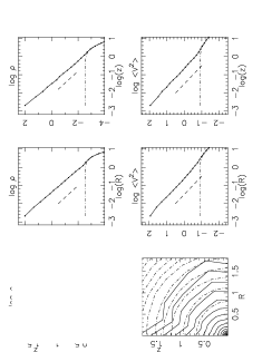
Figure 12: Left: Isocontours for the final density, and profiles along $R$ and $z$, for $M_{BH}/M_{0}=0.2$. Isocontours and profiles for the velocity dispersion are displayed on the second line.

Figure 13: Density profile along $r$ obtained for a BH with final mass resp. $0.05,0.15,1.$ times the initial core mass

6 Cusps in rotating systems

In this section, we investigate the effects of an initial rotation of the host galaxy. LG89 and CB94 both study the rotation brought to central regions by a growing cusp, but find different results. Is the galaxy response somehow affected in these works by the approximation of a spherical potential? Here we can study this case in its true geometry, without any such approximation. Moreover, we would like to clarify which difference in these works is responsible for the difference in the final velocity field. The net rotation within the influence radius is weak in CB94, unless the BH has a mass much larger than the initial core mass. On the other hand, LG89 obtain a cusp in the rotation velocity for any initial BH mass. We therefore investigate in turn models that are built similarly to those considered by CB94, and LG89.

Table 4: List of numerical experiments with rotating models. See Table 3 for the symbols definition. The results are shown for $p=p_{1}(E,L_{z})$; experiments with $p=p_{2}(E,L_{z})$ yield practically identical measures for the logarithmic slopes of both $\rho$ and $\sigma^{2}$.

$\begin{array}[]{c}M_{BH}\\ \hline\cr M_{0}\end{array}$ $\begin{array}[]{c}M_{BH}\\ \hline\cr M_{core}\end{array}$ $\begin{array}[]{c}T_{grow}\\ {\rm(Yrs)}\end{array}$ $\gamma_{\rho}$ $\gamma_{\sigma^{2}}$ $||M_{1}||$ F_max $\begin{array}[]{c}M_{1}\\ \hline\cr||M_{1}||\end{array}$ 0.01 0.05 $10^{7}$ $1.48\pm 0.1$ $0.9\pm 0.1$ $0.02$ 0.01 $0.02$ 0.03 0.15 $10^{7}$ $1.53\pm 0.04$ $0.92\pm 0.1$ $0.05$ $0.02$ 0.03 0.2 1 $10^{7}$ $1.66\pm 0.04$ $1.01\pm 0.03$ 0.4 0.08 $-0.02$

6.1 Models with $p_{1}(L_{z})$

We first experiment with rotating models built using $p(E,L_{z})=p_{1}(L_{z})$ (Eq. 11). The motivation for considering this kind of rotation tapering for small $L_{z}$, is obviously its simplicity. Furthermore, such models are not unplausible if a galaxy has formed through a major merger. Violent relaxation in the central regions can erase net rotation for very bound orbits, whereas less bound orbits may still exhibit a preference for one sense of rotation. An example of merger remnant with this sort of angular momentum distribution is found in numerical simulations by Barnes & Hernquist (1996; their Fig. 17).

The parameters in $p_{1}$ have been chosen as follows:

$$L_{m}=0.2\,l_{0}~{}~{}~{}~{}~{}~{}~{}~{}\eta=0.5.$$ (27)

Figure 14: Initial rotation velocity profile along the $R$ axis, for the model with resp. $p=p_{1}$ (solid line), and $p=p_{2}$ (dashed line), as given by Eq. 11

The corresponding rotation curve is displayed on Fig. 14.

For each BH mass considered, the slope of the cusp is the same, within the error bars, as in the corresponding non-rotating case. These results are summarized in Table 4.

The initial distribution $f_{0}(E_{0},L_{z})$ is displayed on the middle panel of Fig. 15, for a mass ratio $M_{BH}/M_{0}=0.01$, corresponding to $M_{BH}/M_{core}\simeq 0.05$. Again, even for this small final BH mass, the distribution function exhibits little noise. Preference for the positive sense of rotation is reflected by the distortion of the surface $f_{0}(E_{0},L_{z})$, which is higher for $L_{z}>0$ values.

The left panel of Fig. 15 shows the perturbation $f_{1}$ as a function of the initial integrals of motion $E_{0},L_{z}$. The grey shades and contour lines are as in the left panel of Fig. 9. Again, perturbation is strongest for large $E_{0}$ values, and small $L_{z}$ values. The peak of positive perturbation (at $E\simeq E_{0}$) is roughly even in $L_{z}$, corresponding to an energy range where the initial distribution $f_{0}$ is itself roughly even in $L_{z}$. We have indeed considered a model like the model in CB94, where the net rotation is mainly due to orbits having $L_{z}\geq L_{0}$, with $L_{0}$ some finite value. For orbits with high binding energy, $L_{c}(E)$ is smaller than $L_{0}$, so that practically none of them can contribute to the net rotation. On the other hand, for smaller energies $E_{0}$, the perturbation $f_{1}$ is odd with respect to $L_{z}$. This is a consequence of the odd term $\eta p(L_{z})$ that has been added to the distribution function $f_{0}$ in order to construct $f_{0}^{r}$ – see Eq. 8.

The final total distribution function $f(E,L_{z})$ is displayed on the same figure (right panel). At high energies, the distortion of this surface towards positive $L_{z}$ has slightly decreased in amplitude, corresponding to the negative perturbation $f_{1}$ for the positive $L_{z}$. The strip of particles having $E>\Phi_{0}(0)$ is very narrow around $L_{z}=0$, as can be best seen on the grey scale map on top of the right panel. Thus, only orbits with $L_{z}\simeq 0$ become bound to the cusp. As a consequence, orbits confined to the central regions do not create a significant global rotation.

                                                                                           

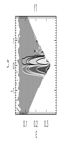
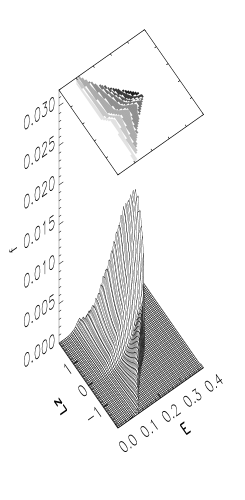
Figure 15: Distribution functions for the case $M_{BH}/M_{0}=0.01$ with rotation, and $p=p_{1}$. The three panels are as in Fig. 9, displaying respectively $f_{1}(E_{0},L_{z})$ (left), $f_{0}(E_{0},L_{z})$ (middle) and $f(E,L_{z})$(right). The grey scales and contour lines used for the left panel are defined as in Fig. 9

Fig. 16 shows the rotation at the end of the BH growth for different mass ratios. Similar to results by CB94, we find that a moderate BH mass does not bring a significant rotation within the influence radius. This result therefore was not affected by simplifications in the analytical derivation of CB94. Our results are indeed very close to those of CB94, as can be seen by comparing our Fig. 16 and their Fig. 3.

As the BH mass increases well above the core mass, its influence radius eventually overcomes the radius corresponding to the circular orbit with angular momentum $L_{0}$, and rotation becomes more important in the centre. However, for the mass ratios we consider (up to $M_{BH}/M_{core}\sim 1$), we find that no cusp is produced in the rotation velocity.

Figure 16: Rotation velocity profiles, along the $R$ axis, for three different mass ratios $M_{BH}/M_{core}=0.05,0.15,1$, as labeled; the dotted line shows the initial rotation of the model

6.2 Models with $p_{2}(E,L_{z})$

We now experiment with a rotating model that uses $p(E,L_{z})=p_{2}(L_{z}/L_{c}(E))$ given by Eq. 11. This model is similar to that by LG89, with their parameter $\omega$ corresponding roughly to $\pi/(2x)$ in our models. We obtain a model with an initial rotation very close to the rotation for the models with $p_{1}$ previously considered, by taking:

$$x=0.2,~{}~{}~{}~{}~{}~{}~{}\eta=0.5.$$ (28)

The corresponding rotation profile along the $R$ axis can be seen on Fig. 14.

In the models now considered, an identical fraction of orbits, at any energy level, contributes to the net rotation. Orbits having initially $E\approx\Phi_{0}(0)$ have $L_{c}(E)\approx 0$, so that even orbits with very small values of $L_{z}$ contribute to the net rotation. These orbits are those which will bring rotation within the cusp. A map for $f_{1}(E_{0}(t=0),L_{z})$ (see §5.5), displayed on Fig. 17, shows indeed that, for orbits with high initial energies, the perturbation has grown positive for $L_{z}>0$, and negative for $L_{z}<0$. Therefore a rotational velocity has efficiently built within the cusp.

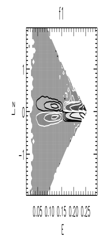
Figure 17: Perturbation distribution function $f_{1}$ as a function of the initial energy $E_{0}$ and $L_{z}$, for the case $M_{BH}/M_{0}=0.01$ with rotation, and $p=p_{2}$.

The effects on the final distribution function are best seen from Fig. 18. We have plotted the case with$M_{BH}/M_{0}=0.03$, rather than the standard case with $M_{BH}/M_{0}=0.01$, because the structure within the total final d.f. is more easily visible. The fact that rotation has been dragged within the density cusp is disclosed by the bent of the surface strip of particles with high binding energies.

This explains why a cusp in rotation velocity is now produced for any BH mass considered, in agreement with the models described by LG89. The cusp follows from the fact that, initially, rotation was present at all levels of energy, including high energies. The rotation velocity profiles along the $R$ axis are shown on Fig. 19, for different masses of the BH. The different curves are labeled as in Fig. 16.

Therefore we have shown that the rotation in the cusp region depends on the orbital structure that existed in the galaxy prior to the BH growth. The formation of a cusp in $V_{rot}$ around a BH that grows adiabatically is sensitive to the way the initial d.f. depends on $L_{z}$. If rotation is not present initially at high binding energies, only very massive BHs –with respect to the initial core mass – will produce an observable signature onto the $V_{rot}$ profile.

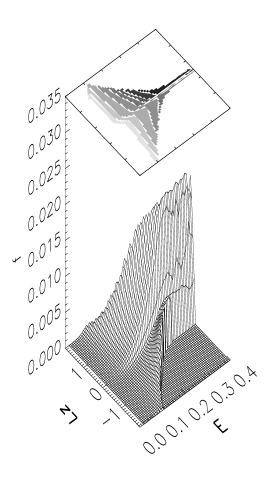
Figure 18: Final total distribution functions for the case with rotation, and $p=p_{2}$; the case with $M_{BH}/M_{0}=0.03$ is shown, for greater legibility.

Figure 19: Same as Fig. 16, but for an initial model with $p(E,L_{z})=p_{2}$ – see text. The label next to each curve refers to the mass ratio $M_{BH}/M_{core}$.

There has been some debate about the role played by a nuclear disk onto the light profile in the center of E galaxies (see Jaffe et al. 1994, and Lauer et al. 1995). Such a disk would of course demand a different model for the rotation profile. The suggestion that the power-law galaxies (those with steep cusps) owed their inner luminosity profile to the presence of a disk has been much weakened by the fact that Lauer et al. (1995) find little evidence for inner disks in the power-law E’s of their sample. More evidence for central disks, at the scale of $\sim 10$ pc, has been collected for SO galaxies (van den Bosch et al. 1994, Scorza & van den Bosch 1998), or giant E’s with shallow cusps (Forbes 1994). Obviously the statistics on the detection of such disks is still too small, and the dynamical models far from entering such detail.

7 Conclusion

This paper aims at investigating the cusp induced in elliptical galaxies by the growth of a central, supermassive black hole. The spherical case is the only one to have been studied in detail in the literature previously, using an adiabatic model. In this paper we study the cusp due to a growing BH by numerical means, in order to free ourselves from the assumption of spherical symmetry.

We thus investigate the possible influence of flattening and rotation, by considering a simple axisymmetric model. For our models, which have a substantial central flattening, we do not find any sizeable signature on the cusp slope with respect to the spherical case. We deduce from this result that a reasonable degree of tangential anisotropy in the stellar velocities, which sustains the flattening, has little effect on the cusp slope. The spherical adiabatic models appear very robust with respect to the geometry of the initial galaxy. We find a cusp slope of $1.5$ in the models where the BH mass is less than the initial core mass, whereas the observed preferred value for low mass E’s is larger, around $1.9$. This fact remains to be explained. One possibility is that the BH grew in a galaxy with initially a very small core, as suggested by van der Marel (1999), or even no core at all. The observational trends (steeper cusps for low luminosity E galaxies, and smaller cores for less massive core Ellipticals) are roughly consistent with this suggestion (see van der Marel 1999). Violent relaxation during a merger or a gravitationnal collapse favours highly concentrated systems (Farouki et al. 1983; see also Chavanis & Sommeira 1998), specially if dissipation occurs (Udry 1993). Gas or stellar collisions around the BH may also have favoured steeper cusps in low $L$ galaxies. The relaxation time is indeed shorter for less massive E galaxies as they have denser centers (cf. Magorrian & Tremaine 1999) and we know that the cusp induced in a collisional system is higher than in the collisionless models, with $\gamma_{\rho}$ around $7/4$ (cf. Duncan & Shapiro 1983).

The formation of a cusp in $V_{rot}$ around a BH that grows adiabatically appears sensitive to the way the initial d.f. depends on $L_{z}$. If rotation is not present initially at high binding energies, only very massive BHs will produce a signature in the $V_{rot}$ profile. Such an initial orbital distribution could for instance be expected after mergers involving an efficient violent relaxation in the central region. Stellar kinematic observations with the required resolution are extremely scarce, although STIS observations (e.g. Joseph et al. 2000) may soon improve on this situation. Existing data for M32 (Joseph et al. 2000) and for the E5 galaxy NGC3377 (Kormendy et al. 1998) show an increase of rotation velocity within the inner few arcsec. This is again consistent with the interpretation that in power-law elliptical galaxies the BH mass exceeds the initial core mass (eventually zero).

On the other hand, a cusp in rotation is produced, whatever the BH/core mass ratio, when initially the fraction of orbits contributing to rotation is non-zero at high binding energies. Evidence for such a cusp is probably present in HST observations of the SO galaxy NGC 4342 (Cretton & van de Bosch 1999).

Let us finally note that the spherical adiabatic model yields values for the mass of dark matter concentration similar to more elaborate dynamical modeling (van der Marel 1999). This however does not preclude that central BHs pre-existed to their host galaxy formation, since the adiabatic growth scenario predicts final galaxy models very similar to those produced by violent relaxation around a pre-existing BH (as demonstrated by Stiavelli 1998, and by our own results on the distribution function).

Acknowledgments

We are grateful to J.-C. Lambert for his extremely efficient and cheerful help with implementing the code on the GRAPE machines. We thank P.-H. Chavanis and A. Bosma for stimulating discussions. F.L. acknowledges gratefully a Marie-Curie fellowship, as well as hospitality at the Marseille observatory, during this work. We would also like to thank IGRAP, the INSU/CNRS and the University of Aix-Marseille I for funds to develop the computing facilities used for the calculations in this paper.

References

Athanassoula, E., Bosma, A., Lambert, J.-C., Makino, J., 1998 MNRAS  293, 369

Barnes, J., Hernquist, L. 1996, ApJ  471, 115

Bender, R. et al. 1989, A&A  217, 35

Binney, J., Tremaine, S. 1987. ‘Galactic Dynamics’, Princeton Univ. Press, Princeton, NJ

Chavanis, P.-H., Sommeira, J. 1998, MNRAS  296, 569

Cipollina, M., Bertin, G. 1994, A&A  288, 43 (CB94)

Cretton, N., van den Bosch, F. C. 1999, ApJ  514, 704

Dejonghe, H. 1986,Phys. Rep., 133, 218

Dejonghe, H., de Zeeuw, T. 1988, ApJ  329, 720

Dehnen, W. 1995, MNRAS  274, 919

Dehnen, W., Gerhard, O. 1994, MNRAS  268, 1019-1032.

Duncan, M. J., Shapiro, S. L. 1983, Nature  262, 743

Duncan, M. J., Levison, H. F., Lee, M.-H. 1998, AJ  116, 51

Evans, N. W. 1994, MNRAS  267, 333-360.

Farouki, R., Shapiro, S., Duncan, M. 1983, ApJ  265, 597

Forbes, D. A. 1994, AJ  107, 2017

Gebhardt, K. et al. 1996, AJ  112 , 105

Gerhard, 0. & Binney, J. 1985, MNRAS  216, 467

Goodman, J., Binney, J. 1984, MNRAS  207, 511

Haehnelt, M. G., Rees, M. J. 1993, MNRAS  263, 168

Hernquist, L., Ostriker, J. P., ApJ  386, 362

Hockney, R., W., Eastwood, J. W., 1981. ‘Computer Simulations Using Particles’, McGraw-Hill

Hunter, C, Qian, E. 1993, MNRAS 262, 401

Jaffe, W., Ford, H. C., O’Connell, R. W., van den Bosch, F. C., Ferrarese, L. 1994, AJ  108, 1567

Joseph, C. L., Merritt, D., Olling, R., Valluri, M. et al. 2000 in preparation

Kawai, A., Fukushige, T., Taiji, M., Makino, J., Sugimoto, D. 1997, PASP  49, 607

Kormendy, J. 1988. In ‘Supermassive Black Holes’, ed. M. Kafatos (Cambridge: Cambridge Univ. Press)

Kormendy, J., Bender, R., Evans, A. S., Richstone, D. 1998, AJ 115, 1823

Kormendy, J., Richstone, D. 1995, ARA&A 33, 581

Lauer, T. et al. 1995, AJ 110, 2622

Lee, M. H., Goodman, J. 1989, ApJ 343, 594 (LG89)

Leeuwin, F., Combes, F., Binney, J. 1993, MNRAS 262, 1013

Leeuwin, F., Dejonghe, H. 1998. In ‘Galaxy Dynamics’, ed. D. Merritt, M. Valluri & J. Sellwood (ASP Conf. Series)

Lynden-Bell, D., 1962, MNRAS 123, 457

Lynden-Bell, D., 1967, MNRAS 136, 101

Magorrian, J., Tremaine, S. 1999, MNRAS 309, 447

Makino, J., Ebisuzaki, T. 1996, ApJ 465, 527

Makino, J., Taiji, M., Ebisuzaki, T., Sugimoto, D. 1997, ApJ 480, 432

Merritt, D. 1998. In ‘Galaxy Dynamics’, ed. D. Merritt, M. Valluri & J. Sellwood (ASP Conf. Series)

Merritt, D., Quinlan, G. 1998, ApJ 498, 625

Nakano, T., Makino, J. 1999, ApJ 510, 155

Nieto, J.-L., Bender, R. 1989, A&A 215, 266

Norman, C.A., May, A., van Albada, T. S. 1985, ApJ 296, 20

Peebles, P. J. E. 1972, Gen. Rel. Grav. 3, 61

Press, W. H., Flannery, B. P., Teukolsky, S. A., Vetterling, W. T., 1986. ‘Numerical Recipes’, Cambridge Univ. Press

Quinlan, G. D., Hernquist, L. 1997, New Ast. 2, 533

Quinlan, G. D., Hernquist, L., Sigurdsson, S. 1995, ApJ 440, 554

Richstone, D. et al. 1998, Nature 395, 14

Saha, P., Tremaine, S. 1992, AJ 104, 1633

Scorza, C., van den Bosch, F. C. 1998, MNRAS 300, 469

Sigurdsson, S., Hernquist, L., Quinlan, G. D. 1995, ApJ 446, 75-85.

Stiavelli, M. 1998, ApJ 495, 91

Tremaine, S. 1997. In ‘Unsolved Problems in Astrophysics’, ed. J. Ostriker (Princeton)

Tremaine, S. et al. 1994, AJ 107, 634

Udry, S. 1993, A&A 268, 35

van den Bosch, F. C., Ferrarese, L., Jaffe, W., Ford, H., O’Connell, R. W. 1994, AJ 108, 1579

van der Marel, R. P. 1999, AJ 117, 744

van der Marel, R. P. 1997. In ‘Galaxy Interactions at Low and High Redshift’, IAU Symp. 186, eds. D. Sanders & J. Barnes (Kluwer)

van der Marel, R., de Zeeuw, T., Rix, H.-W. 1997, ApJ 488, 702

Wachlin, F. C., Rybicki, G. B., Muzzio, J. C. 1993, MNRAS 262, 1007

Wisdom, J., Holman, M. 1991, AJ 102, 1528

Young, P. 1980, ApJ 242, 1232