The Redshift Distribution of FIRST Radio Sources at 1 mJy

Abstract

We present spectra for a sample of radio sources from the FIRST survey, and use them to define the form of the redshift distribution of radio sources at mJy levels. We targeted 365 sources and obtained 46 redshifts (13 per cent of the sample). We find that our sample is complete in redshift measurement to R $\sim 18.6$, corresponding to $z\sim 0.2$. Galaxies were assigned spectral types based on emission line strengths. Early-type galaxies represent the largest subset (45 per cent) of the sample and have redshifts $0.15\la z\la 0.5$ ; late-type galaxies make up 15 per cent of the sample and have redshifts $0.05\la z\la 0.2$; starbursting galaxies are a small fraction ($\sim 6$ per cent), and are very nearby ($z\la 0.05$). Some 9 per cent of the population have Seyfert1/quasar-type spectra, all at $z\ga 0.8$, and there are 4 per cent are Seyfert2 type galaxies at intermediate redshifts ($z\sim 0.2$).

Using our measurements and data from the Phoenix survey (Hopkins et al., 1998), we obtain an estimate for $N(z)$ at $S_{1.4\rm{GHz}}\geq 1$ mJy and compare this with model predictions. At variance with previous conclusions, we find that the population of starbursting objects makes up $\la 5$ per cent of the radio population at S $\sim 1$ mJy.

1 INTRODUCTION

An accurate definition of the redshift distribution of radio sources at faint flux densities has become particularly important in the last decade for both radio astronomy and cosmology. It is critical, for example, in testing radio-source unification (e.g. Jackson & Wall, 1998), and in large-scale structure studies (e.g. Loan et al. 1997, Magliocchetti et al. 1999) to permit the conversion of angular clustering estimates to the spatial clustering estimates required to evaluate structure formation models.

Classical large-scale-structure studies have used wide-area optical and IR surveys to measure the clustering of galaxies, but these are limited to low redshifts, with a peak redshift selection of $\la 0.1$ (e.g. APM, Maddox et al., 1990; IRAS, Fisher et al., 1993). Deep small-area surveys such as the Hubble Deep Field North (Williams et al., 1996) or the CFRS survey (Lilly et al., 1995) have been used to measure clustering to much higher redshifts (see e.g. Le Fevre et al., 1995; Magliocchetti & Maddox, 1998), but they probe small volumes and can measure clustering only on small scales ($\la 1$ Mpc). On the other hand radio objects are detected to high redshifts ($z\sim 4$) and sample a much larger volume for a given number of galaxies, so that they have the potential to provide information on the growth of structure on large physical scales. Recently, clustering statistics in deep radio surveys have been measured (Cress et al., 1997; Loan et al., 1997; Baleisis et al., 1997; Magliocchetti et al., 1998) and these analyses have shown radio sources to be reliable tracers of the mass distribution, even though they may be biased (Magliochetti et al., 1999).

However the relationship between angular measurements and the physically meaningful spatial quantities is highly uncertain without an accurate estimate of the redshift distribution of radio objects $N(z)$ (Magliocchetti et al., 1999). The current estimates of $N(z)$ for radio sources at mJy levels are largely based on predictions from the local radio luminosity functions and evolution (see e.g. Dunlop & Peacock, 1990), and are poorly defined.

Indeed the predictions require the knowledge of more than one luminosity function. Deep radio surveys (Condon & Mitchell, 1984; Windhorst et al., 1985; Fomalont et al., 1993) have shown a flattening of the differential source count $\frac{dN}{dS}$ below S $\sim 10$ mJy. This flattening is generally interpreted as due to the presence of a population of radio sources differing from the radio AGN which dominate at higher flux densities. Condon (1984) suggested a population of strongly-evolving normal spiral galaxies, while others (Windhorst et al., 1985; Danese et al., 1987) claimed the presence of an actively star-forming galaxy population. Observations supported this latter suggestion; the identifications of many of the faint sources are with galaxies with spectroscopic and photometric properties similar to ‘IRAS galaxies’ (Franceschini et al., 1988; Benn et al., 1993). The model predictions of $N(z)$ at faint flux densities from the luminosity functions of Dunlop & Peacock (1990) diverge greatly because of inadequate definition of the radio AGN luminosity functions; but in addition the contribution to $N(z)$ of the starburst population needs consideration.

In order to define $N(z)$ and the population mix at mJy levels, we have observed radio sources from the FIRST survey (Becker et al., 1995) using the WYFFOS multi-object spectrograph on the William Herschel Telescope in 8 1-degree diameter fields. We show how these observations constrain both the form of $N(z)$ and the population mix at S $\sim 1$ mJy for $z\la 0.3$. Section 2 of the paper introduces this radio sample, while Sections 3 and 4 describe acquisition and reduction of the data. In Sections 5, 6 and 7 we present the radio, spectroscopic and photometric properties of the sample. Section 8 is devoted to the analysis of the observed $N(z)$ and comparison with models; the conclusions are in Section 9.

Figure 1: Area covered by the 8 observed fields. Crosses are for the radio sources while open circles show the positions of the optical fibres.

2 THE RADIO DATA

The FIRST (Faint Images of the Radio Sky at Twenty centimetres) survey (Becker, White and Helfand, 1995) began in the spring of 1993 and will eventually cover some 10,000 square degrees of the sky in the north Galactic cap and equatorial zones. The VLA is being used in B-configuration to take 3-min snapshots of 23.5-arcmin fields arranged on a hexagonal grid. The beam-size is 5.4 arcsec at 1.4 GHz, with an rms sensitivity of typically 0.14 mJy/beam. A map is produced for each field and sources are detected using an elliptical Gaussian fitting procedure (White et al., 1997); the $5\sigma$ source detection limit is $\sim$1 mJy. The surface density of objects in the catalogue is $\sim 90$ per square degree, though this is reduced to $\sim 80$ per square degree if we combine multi-component sources (Magliocchetti et al., 1998). The depth, uniformity and angular extent of the survey are excellent attributes for investigating the clustering properties of faint sources.

We used the 4 April 1998 version of the catalogue which contains approximately 437,000 sources and is derived from the 1993 through 1997 observations covering nearly 5000 square degrees of sky, including most of the area $7^{h}20^{m}<{\rm RA}(2000)<17^{h}20^{m}$, $22.2^{\circ}<{\rm Dec}<57.5^{\circ}$ and $21^{h}20^{m}<{\rm RA}(2000)<3^{h}20^{m}$, $-2.5^{\circ}<{\rm Dec}<1.6^{\circ}$. This catalogue has been estimated to be 95 per cent complete at 2 mJy and 80 per cent complete at 1 mJy (Becker et al., 1995).

3 OBSERVATIONS

3.1 Field Selection

For the purpose of determining the redshift distribution, the precise position of the fields is not crucial, although several factors were taken into account when choosing which to observe. The fields must span a range of RA’s to ensure they could be observed at low zenith distance throughout the allocated nights. The fields are at as high galactic latitude as possible to reduce the probability of confused optical identifications and to ensure low galactic extinction (the allocated time meant the fields had to be on opposite sides of the galactic plane). We also cross-checked with fields which will be observed as part of the INT Wide-Field Camera survey, and chose our fields to overlap with these, so that deep optical images will be available in the near future.

These constraints lead to the choice of three main areas: $16^{h}11^{m},\;+54^{\circ}22^{\prime}$ (which covers the ISO ELAIS field); $22^{h}40^{m},\;+0^{\circ}0^{\prime}$, and $02^{h}30^{m},\;+0^{\circ}0^{\prime}$. We also observed a field adjacent to the ELAIS field, and one on each side of the $22^{h}40^{m},\;+0^{\circ}0^{\prime}$, and $02^{h}30,\;+0^{\circ}0^{\prime}$ fields. The areas actually observed are shown in Figure 1, and the field centres are listed in Table 1.

3.2 WYFFOS and AUTOFIB2

The 4.2-m William Herschel Telescope (WHT) has a prime-focus corrector with an atmospheric-dispersion compensator that provides a field of view of one degree in diameter. AUTOFIB2 is a robotic positioner, which places up to 120 optical fibre feeds in the focal plane, each fibre collecting light from a $2.7^{\prime\prime}$ diameter patch of sky. The fibres are fed to WYFFOS which is a multi-object spectrograph, at one of the WHT Nasmyth foci. The spectrograph can use a range of gratings offering 30 - 500 Å/mm dispersion. We chose to use the 600 lines/mm grating with the Tek1024² CCD, which gives a dispersion of $\sim 3$ Å per pixel, and a resolution of $\sim 10$Å. For a central wavelength at 6000Å this set up gives spectra from $\sim 4400$Å to $\sim 7400$Å.

3.3 Astrometry and Fibre Positioning

The fibres on WYFOSS cover 2.7 arcsecs on the sky, but to obtain the best throughput, they must be positioned to an accuracy of $0.5^{\prime\prime}$ or better. The astrometric reference frame of the FIRST survey is accurate to $0.05^{\prime\prime}$, and individual sources have 90% confidence error circles of radius $<0.5^{\prime\prime}$ at the 3 mJy level and $1^{\prime\prime}$ at the survey threshold. This means that, in principle, the radio source positions are accurate enough to position the fibres, even without optically identified counterparts. Using the radio positions means that our sample is not biased towards optically bright sources. Although our spectroscopy will clearly be limited by the optical brightness, it should be possible to obtain redshifts for any sources that have strong optical emission lines but very faint continuum. These sources would have been rejected from the sample if we required every target to have an optical counterpart. However there are a few complications in using the radio positions and these must be taken into account.

First, the telescope must be positioned and guided using fiducial stars. We selected stars with $13<b_{J}<15$ from APM scans of UKST plates for the equatorial fields, and of POSS2 plates for the ELAIS fields. These star positions are accurate to about $0.1^{\prime\prime}$, but have been measured in an optical reference frame, which may be offset from the radio reference frame by more than an arcsecond. Therefore we matched up the radio sources and optical images for each Schmidt plate.

Figure 2 shows a typical plot of the positional residuals between the optical and radio positions. There is a uniform background of points with residuals greater than $1^{\prime\prime}-2^{\prime\prime}$, which come from random coincidences between optical and radio sources. The true optical identifications show up as the concentration of points near zero offset. The mean positional offset of the identifications is $0.9^{\prime\prime}$ in RA and $0.5^{\prime\prime}$ in Dec, corresponding to the offset between the optical and radio astrometric frames, and this offset was applied to each position in the ELAIS field so that the optical and radio astrometry coincide. Similar offsets were calculated for each of the other observed fields. The scatter in residuals about the mean offset is about $0.5^{\prime\prime}$ which is consistent with the quoted positional accuracy of the surveys.

Figure 2: The positional residuals between FIRST radio sources and APM optical positions in the ELAIS field. The points with residuals greater than $1^{\prime\prime}-2^{\prime\prime}$ are likely to be random coincidences and the points with near-zero offset are the true optical identifications. The scatter suggests that the combined rms error between the optical and radio objects is about $0.5^{\prime\prime}$, which is consistent with the quoted errors in each survey. The mean offset is $0.9^{\prime\prime}$ in RA and $0.5^{\prime\prime}$ in Dec.

The second complication is that the optical ID of an extended radiosource will not necessarily lie at the radio catalogue position. In the case of a classical double-lobed radiosource, the radio core and optical ID will lie between the lobes, which themselves may be catalogued as two separate radio sources. In the case of a core-jet radiosource, the radio core and optical ID will usually lie away from the centroid of the radio emission. To address this problem, we extracted $4^{\prime}\times 4^{\prime}$ radio maps from the FIRST database and optical images covering a similar area from the Digital Sky Survey (DSS). We visually inspected each of the radio maps, and overlaid the optical contours so that we could identify possible offsets between the radio and optical emission. Almost all of the radiosources were either unresolved or dominated by an unresolved component in the FIRST maps. Only in a few cases it was necessary to manually adjust the positions. A typical plot showing the FIRST radio map and overlaid optical contours is shown in Figure 3.

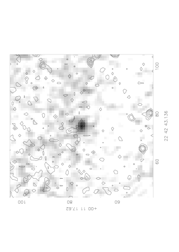
Figure 3: A grey-scale $4^{\prime}\times 4^{\prime}$ radio map of a FIRST source. The overlaid contour map is from the optical DSS image.

As well as the fiducial stars and target objects, it is necessary to observe some regions of blank sky, so that the sky spectrum during the observations can be estimated and subtracted from the target spectra. On average there are 70 radio sources per field (see Table 1), leaving 50 fibres which could be used for sky. Two sets of sky positions were generated for each field. The first set were the target positions in the focal plane when the telescope is offset by 5 arcminutes in Dec. Note that the spherical geometry of the sky means that new positions do not exactly correspond to a simple addition of 5 arcmins to each Dec. The low surface density of bright optical images meant that these positions were blank sky for all but a couple of cases. The second set were simply randomly chosen positions; again most of these are blank sky. Given the large number of sky fibres we could median them together to obtain a highly accurate estimate of the true sky spectrum, even if a few were contaminated by objects.

3.4 Field Configurations

Each fibre for AUTOFIB2 can be placed within a restricted area defined by a maximum radial extension and a maximum tilt angle from the radial direction. Also no fibre can cross another, and there must be a small buffer-zone around each fibre. These constraints limit the number of targets that can be allocated to a fibre within a particular field. The program CONFIGURE is part of the WYFFOS software package, and it attempts to find the most efficient set of target-to-fibre allocations. This configuration was then inspected and some changes were made manually to increase the number of fibres allocated to targets. A typical configuration is shown in Figure 4. The total number of targets and number of fibres allocated is shown in Table 1.

Table 1: Observed fields. $\alpha$ and $\delta$ are respectively the RA and Dec of the field centres. $N_{\rm radio}$ is the number of radio objects in each field, $N_{\rm obs}$ is the number of object-positions on which fibres could be placed and $N_{z}$ is the number of sources with a redshift determination. Note that $N_{\rm radio}$ is the number obtained after combining multiple components into a single source.

Field	$\alpha$ (J2000)	$\delta$ (J2000)	$N_{\rm obs}$	$N_{\rm radio}$	% Configured	$N_{z}$	% Redshifts
F0226	02 28 33.8	+00 13 22	48	78	61.5	3	6.3
F0230	02 32 33.8	+00 13 12	57	86	66.3	4	7.0
F0234	02 34 33.8	+00 13 01	35	55	63.6	1	2.8
F2236	22 38 33.7	+00 15 38	40	53	75.5	10	25
F2240	22 42 33.7	+00 15 44	44	59	74.5	10	23
F2244	22 46 33.7	+00 15 49	50	85	58.8	11	22
ELAIS	16 10 00.0	+54 30 00	49	72	68.0	3	6.1
ELAIS2	10 04 13.0	+54 01 52	42	62	67.7	4	9.5

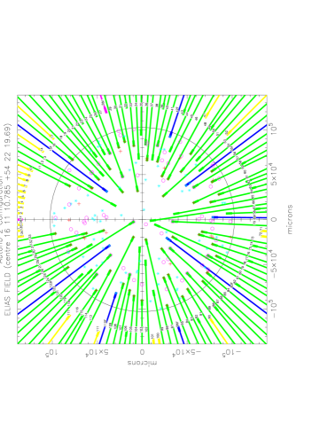
Figure 4: The fibre configuration for a FIRST field. The large circle represents the full - 1 degree - field of view. The dark grey outlines show the positions of fibres for the spectrograph and the black outlines show the fibres for the fiducial stars. Broken or unusable fibres are shown in light grey. The FIRST sources are marked with crosses, and the sky positions are marked by circles.

3.5 Observing Procedure

Once a field has been configured and acquired we took a standard sequence of calibration frames and observations of the target field. The sequence began with an arc lamp for wavelength calibration; then 1800 sec on the targets; then three 600 sec offset sky integrations; another 1800 sec on the targets; another three 600 sec skies; and finally 1800 sec on targets. Each of the offset skies was given a different offset to ensure that the sky spectra were not contaminated by random objects that happen to fall on the fibres.

Most of the targets are very faint, so accurate sky subtraction is crucial. The main aim of the observing sequence is to provide an accurate estimate of the sky spectrum during the observations, and also to calibrate the relative throughputs of each fibre for this particular configuration. Since the field is vignetted, the apparent transmission of a fibre will depend on its position in the field. Also the efficiency of light entering a fibre will depend on the precise angle that the fibre button settled when placed by AUTOFIB2, so there may be small variations even if the fibres are repositioned to the same configuration. This also means that flat-fields from internal lamps will not exactly reproduce the throughputs as seen on the sky. The offset skies are observed with exactly the same set-up as the target objects, and so provide very accurate relative throughput estimates for the object and sky fibres. The large number of sky fibres provides an accurate estimate of the actual sky spectrum during the object integrations.

In principle the $5^{\prime}$ offset skies allow a more efficient observing mode that does not require separate offset sky integrations. If the telescope is nodded back and forth between the target positions, and the offset fibres, light from the targets is always being collected. Also the sky spectrum can be measured through the actual fibre used for each target. The disadvantage of this approach is that a sky fibre must be allocated to each object fibre, and this leads to quite severe configuration constraints. Typically less than 50% of the available targets could be allocated a pair of fibres, and so this turned out to be a rather inefficient option for our project. Nevertheless we did successfully apply the method for one field (F0234).

During daylight we took high signal-to-noise tungsten lamp flat-fields which were used to define the position of each fibre spectrum as described below.

4 Data Reduction

The data obtained were reduced using a package within IRAF written specifically to reduce WYFFOS data. The first steps in the data reduction are the standard bias level subtraction and trimming of the overscan regions. Then the tungsten flat-fields are used to locate and fit polynomials to the spectrum of each fibre. These polynomials allow 1-D spectra to be extracted from the 2-D images. The package uses information in the file headers to ensure the correct link between fibre number and spectrum number, so that each spectrum is identified with the correct input target.

Next, for each target field, the 2-D images from the individual integrations were averaged together, using the IRAF ccdreject option. Similarly the offset skies for each field were combined. This way of combining the images provides good signal-to-noise for pixels where all component images are good data, and effectively rejects pixels contaminated by cosmic rays or random objects that happened to fall in a sky fibre for one particular offset.

As a simple but effective method of sky subtraction, the 2-D averaged offset skies were rescaled to match the exposure time in the target frame and then simply subtracted from the 2-D target data. This technique was used because WYFFOS suffers from light scattered within the spectrograph. The broad scattered light features seen in Figure 5(a) have $\sim 10\%$ of the counts in the actual spectra, and so it is very important to subtract them accurately. The standard approach attempts to fit a smooth 2-D polynomial to the light in between the fibres, and subtracts this from the 2-D data frame. Then 1-D spectra are extracted from the 2-D data, and the sky-fibres are used to define the mean sky spectrum, which is rescaled according to a throughput map generated from offset skies, and subtracted from each object spectrum. We found that it was very difficult to fit the scattered light accurately enough to leave a clean 2-D image with reliable spectra. Since our target galaxies are very faint, the scattered light is almost entirely from the sky, even in the target fields. Therefore simply re-scaling the 2-D offset sky frames and subtracting from the 2-D target frame means the scattered light and the sky are both properly subtracted. This is very effective, as seen in Figure 5(b).

Figure 5: (a) A combined 2-D frame of WYFFOS spectra before sky subtraction. The spectrum from each fibre is dispersed in the vertical direction, and several bright sky emission lines can be seen in each spectrum. Each set of 3 fibres is offset on the slit in a saw-tooth configuration, which gives a vertical shift to the wavelength zero-point of neighbouring spectra. The broad horizontal features are from scattered light in the spectrograph. (b) the sky-subtracted 2-D spectra. Both the sky lines and the scattered light have been subtracted well, but the pattern of the scattered light can be seen as regions of increased noise in the background. Note that the spectra are not perfectly straight, and a polynomial must be fitted to each one in order to properly extract the 1-D spectra.

This sky-subtraction approach is susceptible to errors if the sky is rapidly varying, because the actual sky spectrum during the target integration is not used. Any such errors can be simply corrected by using the spectra from the sky fibres in sky-subtracted 2-D images to estimate the average residual sky which can then subtracted from the target spectra. As can be seen in the spectra, the residuals from sky-subtraction are very small, confirming that the approach works very well.

The wavelength calibration for each data-set was carried out using the standard IRAF tasks. This automatically accounts for the ’saw-tooth’ arrangement of fibres on the spectrograph slit.

5 Spectral Analysis and Classification

5.1 REDSHIFT DETERMINATION

Redshifts were determined in 46 objects, corresponding to $\sim 13$ per cent of the spectroscopic sample. Determinations were obtained in two separate ways: first by visual inspection of the spectra and attempting to identify individual features; second via cross-correlation with a range of templates.

The cross-correlation analysis uses the same algorithm as the 2dF redshift survey code (Seaborne, 2000) but has small changes to the filtering parameters, the wavelength coverage and allowed redshift range appropriate for ou WYFOSS data. The cross-correlation functions between the data and a set of template spectra are calculated and the highest peak is located. An index $0\leq q\leq 4$ is automatically assigned according to the height of the peak and the noise and assesses the quality of the redshift measurement: 0 corresponding to no redshift estimate, and 4 a reliable redshift. Each redshift estimate was also checked by eye at this stage, and the quality flag was updated if necessary. We accepted estimates with $q$ as low as 3, so long as they agreed with the results from visual inspection. A few objects (all absorption systems) with $q=2$ were included in the final sample, when the cross-correlation estimate was in agreement with the results from visual inspection. Table 2 lists the measured redshifts for the observed targets.

5.2 SPECTRAL CLASSIFICATION

The optical counterparts of radio sources with a redshift determination were classified into 6 main groups according to their spectral features:

1. Early-type galaxies where spectra were dominated by continua much stronger than the intensity of any emission lines present. These objects can then be divided into two further categories:

   • Galaxies with absorption lines only.

   • Galaxies with absorption lines + weak but non-negligible OII. emission lines

2. Late-type galaxies showing strong emission lines characteristic of star-forming activity, together with a detectable continuum.

3. Starburst galaxies where the continuum is missing and the spectra only showed strong emission lines due to star-formation activity.

4. Seyfert1 galaxies showing strong broad emission lines. These objects could be quasars.

5. Seyfert2 galaxies showing narrow emission lines due to the presence of an active galactic nucleus. To have an objective classification of the narrow emission line objects and in particular to distinguish Seyfert2’s from galaxies heated by OB stars (classes 2-3), we used the diagnostic emission line ratios of Baldwin, Phillips & Terlevich, 1981 and Rola, Terlevich & Terlevich, 1997.

6. A final class consisted of those objects whose spectra show a detectable continuum but the complete absence of features; no redshift determinations for these were possible. These spectra are generally believed to be associated with early-type galaxies (see Gruppioni, Mignoli & Zamorani, 1998), given the lack of emission lines.

Also, four spectra appear to be stars at zero redshift; these are most likely to be random positional coincidences with galactic stars.

Table 2 lists the spectral classes. All spectra with significant signal are shown in Figure 6. The spectrum at the bottom of each panel show the sky spectrum, with strong emission lines marked. The galaxy spectra have not been flux calibrated, and the line on the lower right is an approximate atmospheric transmission curve, showing the position and shape of the atmospheric A and B absorption bands.

Figure 6: Spectra of all detected sources. Each spectrum is labelled with the object name and redshift where it has been possible to measure it. The spectrum at the bottom of each panel is the sky spectrum, with strong emission lines marked. The galaxy spectra have not been flux calibrated, and the line on the lower right shows an approximate atmospheric transmission curve, in particular showing the position and shape of the atmospheric A and B absorption bands.

Figure 7: continued

Spectra of all detected sources

Figure 8: continued

Spectra of all detected sources

Figure 9: continued

Spectra of all detected sources

6 Photometry

Figure 10: Apparent magnitude R vs. radio flux S_1.4GHz for the objects in the fields as shown in the figure. Filled dots indicate sources with a redshift determination, while circles are for objects with no $z$.

6.1 The APM Survey

Some of the fields (F0226, F0230, F0234, F2236, F2240, F2244) targeted in our WHT observations lie in regions of the sky sampled by the APM scan of UKST plates (http://www.ast.cam.ac.uk/^∼apmcat/). The APM data provided R and B magnitudes of the objects in the sample brighter than B $\sim 22$, R $\sim 21$, the limiting magnitudes of the APM survey.

To obtain these magnitude measurements we searched the UKST catalogue for optical counterparts lying within 2.7 arcseconds from the corresponding radio position. Note that the fibre position always coincides with the radio coordinates except in the case of double sources (see Section 3.3). The tolerance in positional matching allows for measurement errors and the fact that the centre of radio emission might be displaced from the centre of the optical emission, especially if the radio object is extended. If no optical object within this offset was found in the UKST catalogue we assumed the object to be fainter than the limiting magnitude.

A few objects in the F0230 and F2240 fields show a displacement greater than the value of 2.7^′′ (but within 3^′′ - Table 2). These are the sources observed at the MDM Observatory (see Section 6.2).

Figure 10 plots the apparent magnitude R vs. the radio flux S${}_{1.4\,{\rm GHz}}$ for all those sources with an optical counterpart in the APM catalogue. Filled dots represent objects with a redshift determination, while circles are for those objects with no $z$. The plot indicates that the percentage of successful redshift determinations is $100\%$ to R $\sim 18.6$ and then decreases with increasing apparent magnitude at a rate which varies from field to field. Figure 10 also shows that almost all the objects in our spectroscopic sample with a redshift determination are brighter than the APM limiting magnitude; only 3 sources with a measured redshift are not detected in the APM data.

Figure 11: R magnitude versus radio flux at 1.4 GHz (top-left) and redshift $z$ (top-right); B magnitude versus radio flux at 1.4 GHz (bottom-left) and redshift $z$ (bottom-right). Filled dots are for early-type galaxies, filled triangles for late-type galaxies, filled squares for starburst galaxies, open dots for Seyfert1 galaxies / quasars, and stars indicate Seyfert2 galaxies. Crosses correspond to objects with no redshift measurement. The solid lines in the R-$z$ and B-$z$ plots represent the best fit to the data (see text), while the dashed lines in the top-right panel show 2$\sigma$ confidence limits.

6.2 Further observations

CCD observations at the MDM Observatory have yielded R magnitudes ($21<{\rm R}<26$) for objects in the F0230 and F2240 fields as shown in Figure 10 and Table 2 (D. Helfand, private communication).

6.3 Field-to-field scatter

The success rate of redshift determination varied strongly from field to field as shown in Table 1; $N_{obs}$ and $N_{z}$ are respectively the number of observed sources and the number of sources with redshift determinations. The striking differences in redshift success between fields are illustrated in Figure 10; the fields at 22^h have far more redshift determinations than the fields at 02^h, which average only a $\sim 5$ per cent success rate. This region also has an anomalously low number of optical identifications in the FIRST survey (D. Helfand private communication), even though the surface density of radio sources is close to the average.

Comparing the two fields for which we have photometric information down to R $\sim 26$, in the case of F2240, E(B-V)=0.067, while for F0230, E(B-V)=0.027 (D. Helfand, private communication). Thus it is not Galactic extinction that produces the very different identification rates. We are looking at either intergalactic extinction or evidence of large-scale structure.

If we assume that radio galaxies cluster as optical galaxies, we can make a crude estimate of the expected variance in the number of measured redshifts in each WHT field. As discussed later, the typical redshift of galaxies in our sample is $z\sim 0.2$, and so each 1^∘ field samples a volume of roughly $1.7\times 10^{4}h^{-3}$ Mpc³ out to $z=0.2$. Ignoring the difference in shape, this volume is equivalent to a 26$h^{-1}$Mpc cube, for which we would expect a fractional variance in the number of optical galaxies to be between 0.3 and 0.4 (Loveday et al., 1992). The observed field-to-field variance is 0.6, which may reflect the higher clustering amplitude of radio galaxies.

Whatever the true explanation, the observed variation is important in itself because of implications for the number of radio-sources with faint optical continuum but bright emission lines. We return to this issue in Section 8 when estimating $N(z)$.

7 OPTICAL AND RADIO PROPERTIES OF THE SAMPLE

Table 2 shows the properties of objects in our sample for which we have data (either spectroscopic or photometric) on the optical counterpart. The columns are as follows:
(1) Source number.
(2) Right ascension and declination of the targeted object. These coordinates are from those of the FIRST survey except in the case of 2240_004 for which the fibre was placed at the centroid of a double source.
(3) Offset of the optical counterpart in the APM catalogue before correction for sytematic offsets.
(4-5) Apparent magnitudes R and B of the optical counterpart.
(6) Radio flux density at 1.4 GHz.
(7) Redshift.
(8) Spectral classification.
(9) Emission lines detected.

Plots for the subsample with redshift determinations are presented in Figure 11 for (1) R magnitude vs. radio flux, (2) R vs. redshift, (3) B magnitude vs. radio flux, and (4) B vs. redshift. The solid line in the R-$z$ plot of Figure 11 represents the relation

$$R-M_{R}=-5+5{\rm log}_{10}d_{L}(pc)\simeq 25-5{\rm log}_{10}{\rm H}_{0}+$$

$$+5{\rm log}cz+1.086(1-q_{0})z$$ (1)

($d_{L}$ the luminosity distance), obtained by a minimum $\chi^{2}$ fit to the data with the absolute magnitude $M_{R}$ as free parameter. This analysis, for $H_{0}=$ 50 Km sec^-1Mpc^-1 and $q_{0}=0.5$, gives a value of $M_{R}\simeq-23.1$ with little scatter ($\Delta M_{R}\sim 0.5$ at the $2\sigma$ level - dashed lines in Figure 11). There are clearly two populations in the diagram, and to find the best fit for early types we excluded Seyfert-type galaxies and starbursts; the result from using all galaxies was virtually identical. The result is in very good agreement with previous estimates (see e.g. Rixon, Wall & Benn, 1991; Gruppioni, Mignoli & Zamorani, 1998; Georgakakis et al., 1999), showing that passive radio galaxies are reliable standard candles. The solid line in the B-$z$ plane of Figure 11 shows a $\chi^{2}$ fit yielding $M_{B}\simeq-21.3$, although the fit is not as good as that in the R-$z$ plane. The fit is improved if only early-type galaxies are included.

Figure 12 shows radio flux S_1.4GHz vs. redshift for the objects with a redshift determination. Though the number of objects in each class is small, we can see that different classes of objects occupy different regions of the planes in Figures 11 and 12:

• Early-type galaxies are found at intermediate redshifts ($0.1\la z\la 0.6$) and make up the entire spectroscopic sub-sample with $0.2\la z\la 0.5$. Their radio fluxes lie in the range $1\la{\rm S}_{1.4\,{\rm GHz}}\la 10$ mJy and optically they appear as relatively faint objects (R $\ga 17$, B $\ga 18.5$). Their absolute magnitude $M_{R}\sim-23$ is consistent with FRI-type radio galaxies (Ledlow & Owen, 1996).

• Late-type galaxies are found from low to intermediate redshifts ($0.05\la z\la 0.2$) perhaps constituting an intermediate step between early-type and starburst galaxies. Their radio fluxes range from S${}_{1.4\rm{GHz}}\simeq 1.5$ mJy to S${}_{1.4\,{\rm GHz}}\simeq 6$ mJy, with a single exception of one radio-bright object (2236_013, S${}_{1.4\rm{GHz}}=116$ mJy). The B and R magnitudes show intermediate values, $15\la{\rm R}\la 17$ and $15\la{\rm B}\la 19$.

• Starburst galaxies in the sample are very nearby ($z\la 0.05$), optically-bright (R $\la 14$, B $\la 14.5$), and faint in radio emission (S${}_{1.4\,{\rm GHz}}\la 3$ mJy). Two of them (0230_071 and 0230_061) are separated by $\la 1h^{-1}$Mpc and show very similar properties, suggesting that interaction may be responsible for the enhanced star-formation rate.

• Seyfert2 galaxies are found at intermediate redshifts ($z\sim 0.2$) and their radio flux densities are extremely low (S${}_{1.4\,{\rm GHz}}\la 1$ mJy). Photometric data are available for only one. These objects lie close to the line delimiting Seyferts from HII galaxies in the log(OIII/$H\beta$)/log(OII/$H\beta$) plane (Rola, Terlevich & Terlevich, 1997).

• Seyfert1 galaxies / quasars exhibiting broad emission lines are only found at $z\ga 0.9$. These objects are very bright in the radio but quite faint in both the R and B bands. 2240_004 is a double source showing characteristic radio lobes symmetric with respect to the optical centre (which does not show a radio core).

• Unclassified objects. These are probably early-type galaxies since they occupy the region in the R-S and B-S planes which is occupied by early-type objects. Also their colours are consistent with them being red/old objects; almost 50 per cent of objects this subsample have R magnitudes (with $18.6\la{\rm R}\la 20$) in the APM catalogue but no B magnitudes, because they are below the APM survey limit. For these objects we used the R-$z$ relation of Figure 11 to estimate redshifts. The corresponding values are given in Table 2, distinguished by asterisks. (Note that we do not use these redshift estimates in the following analysis.)

Table 2: Observed FIRST sources. Where an APM optical identification was found the offset from the radio position, and R and B magnitudes are listed. The measured redshifts and spectral type are listed for the targets detected in the spectral data.

Object	$\alpha$ (J2000)	$\delta$ (J2000)	Offset [$\prime$$\prime$]	R	B	S1.4 [mJy]	z	Class	Emission Lines
0226_041	2 29 53.551	+00 2 18.53	$0.68$	$18.8$	$21.3$	$1.24$	$0.369$	Early	none
0226_068	2 30 21.753	+00 5 11.21	$2.66$	$9.5$	$11.4$	$5.77$	$0.0$	Star	none
0226_063	2 30 14.969	+00 22 39.30	$0.59$	$20.0$	$>22$	$3.25$	0.246	Early	OII
0230_048	2 33 5.021	+00 32 39.60	?	$>26$	$>22$	$3.2$	$0.393$	Early	OII
0230_071	2 32 47.492	+00 40 40.85	$0.38$	$14.2$	$13.4$	$0.96$	$0.023$	SB	H${\gamma}$,H${\beta}$,OIII,H${\alpha}$
0230_063	2 31 28.228	-00 7 34.35	$0.53$	$18.8$	$20.9$	$0.95$	$0.2873$	Early	OII
0230_061	2 31 37.698	-00 8 23.57	$0.18$	$10.0$	$11.5$	$3.27$	$0.02$	SB	H${\gamma}$,H${\beta}$,OIII,H${\alpha}$
0230_018	2 33 2.830	+00 24 5.90	?	$>26$	$>22$	$3.8$	?	?
0230_006	2 32 47.092	+00 19 50.46	$2.8$	$25$	$>22$	$2.43$	?	?
0230_029	2 32 28.230	+00 27 44.27	?	$>26$	$>22$	$3.08$	?	?
0230_066	2 31 57.592	+00 38 54.68	$0.71$	$19.7$	$>22$	$2.48$	$\sim 0.53^{\ast}$	Unclass	none
0230_037	2 32 6.979	+00 28 45.46	$1.3$	$23.5$	$>22$	$3.5$	?	?
0230_023	2 32 7.959	+00 25 26.69	?	$>26$	$>22$	$1.48$	?	?
0230_009	2 32 9.710	+00 22 36.90	?	$>26$	$>22$	28.56	?	?
0230_054	2 31 5.596	+00 8 44.00	0.91	20	20.7	55.01	?	?
0230_002	2 32 29.895	+00 12 1.97	?	$>26$	$>22$	1.47	?	?
0230_031	2 32 9.524	-00 1 28.66	?	$>26$	$>22$	1.24	?	?
0230_041	2 32 16.497	-00 4 45.56	?	$>26$	$>22$	3.10	?	?
0230_008	2 32 28.662	+00 2 33.72	$1.4$	24.9	$>22$	1.74	?	?
0230_025	2 32 32.444	-00 0 44.07	2.4	21.7	$>22$	2.21	?	?
0230_067	2 33 13.848	-00 12 14.83	1.11	18.6	19.5	5.9	$\sim 0.33^{\ast}$	Unclass	none
0230_010	2 32 52.548	+00 2 34.79	1.4	20.8	$>22$	41.56	?	?
0230_014	2 33 0.332	+00 2 35.44	?	$>26$	$>22$	0.69	?	?
0230_013	2 33 8.894	+00 4 42.19	$1.8$	24.6	$>22$	1.85	?	?
0230_028	2 33 31.030	+00 10 23.61	0.94	18.4	20.3	4.59	$\sim 0.31^{\ast}$	Unclass	none?
0230_026	2 33 30.170	+00 14 48.03	1.4	21.9	$>22$	2.06	?	?
0230_011	2 33 15.494	+00 18 34.54	0.0	21.9	$>22$	3.62	?	?
0234_026	2 35 11.618	+00 6 8.29	?	$>21$	$>22$	5.39	0.328	Early	none
0234_051	2 37 3.870	+00 39 23.88	0.9	20.1	20.5	1.8	?	?
0234_005	2 36 9.341	+00 18 57.04	0.28	18.8	21.0	2.46	$\sim 0.36^{\ast}$	Early	none?
0234_041	2 34 57.578	+00 21 30.49	0.41	20.1	21.0	3.72	?	?
2236_005	22 38 45.422	+00 8 39.11	0.23	19.1	21.8	5.52	0.317	Early	OII
2236_012	22 39 32.234	+00 12 42.49	1.77	16.7	17.8	1.46	0.161	Late	H${\beta}$,OIII
2236_001	22 38 43.562	+00 16 48.15	0.29	19.0	20.5	37.54	3.44	Sy1	Ly${\alpha}$,CIV
2236_023	22 39 8.156	+00 32 32.09	0.79	18.0	20.2	4.29	0.213	Late	OIII
2236_008	22 38 2.438	+00 23 34.55	0.1	18.4	20.2	0.40	0.201	Sy2	OII,OIII
2236_013	22 37 37.117	+00 20 39.02	0.1	16.4	18.6	115.99	0.195	Late	OII,OIII
2236_009	22 37 49.289	+00 19 0.85	0.22	16.1	17.8	1.02	0.116	Early	none
2236_034	22 36 51.883	+00 12 23.11	0.72	16.9	18.9	1.48	0.191	Early	none
2236_016	22 37 28.898	+00 10 1.02	?	$>21$	$>22$	66.11	0.0	Star	none
2236_046	22 37 6.594	-00 2 31.66	1.2	15.3	17.4	9.33	0.161	Early	none
2236_028	22 39 18.391	-00 4 34.18	0.23	19.9	$>22$	1.83	$\sim 0.50^{\ast}$	Unclass	none?
2240_002	22 42 22.117	+00 15 5.80	0.3	19.6	20.6	17.33	1.35	Sy1	CIII,MgII
2240_008	22 42 12.805	+00 8 12.71	0.69	20.1	$>22$	2.64	0.515	Early	none
2240_023	22 42 12.055	+00 2 11.83	0.81	19.1	21.6	1.71	0.433	Early	none
2240_004	22 42 43.141	+00 11 17.62	?	$>26$	$>22$	4.11	0.35	Early	none
2240_038	22 44 4.414	+00 12 16.71	0.43	18.9	21.2	12.49	0.359	Early	none
2240_016	22 43 22.695	+00 15 21.01	0.5	17.9	21.1	4.21	0.29	Early	none
2240_033	22 43 38.438	+00 25 17.64	1.82	16.8	19.3	2.36	0.175	Early	OII,OIII
2240_021	22 43 15.477	+00 24 28.93	1.43	14.1	14.6	1.83	0.057	SB	H${\gamma}$,H${\beta}$,OIII,H${\alpha}$
2240_010	22 42 27.078	+00 25 57.40	0.55	19.1	$>22$	1.77	0.319	Early	none
2240_014	22 41 46.367	+00 16 8.19	0.54	20.4	20.4	43.96	1.49	Sy1	CIII,MgII
2240_040	22 41 45.398	-00 4 1.12	1.9	25.6	$>22$	4.05	?	?
2240_011	22 42 15.273	+00 6 19.84	0.0	21.7	$>22$	4.96	?	?
2240_050	22 41 46.234	-00 8 44.18	?	$>26$	$>22$	2.96	?	?
2240_042	22 42 10.977	-00 6 57.91	1.4	$>26$	$>22$	2.99	?	?
2240_006	22 42 33.227	+00 8 58.03	?	$>26$	$>22$	1.30	?	?
2240_005	22 42 51.148	+00 11 43.35	1.78	18.6	20.9	5.08	$\sim 0.33^{\ast}$	Unclass	none
2240_025	22 43 34.125	+00 8 46.66	?	$>26$	$>22$	3.40	?	?
2240_024	22 43 38.047	+00 17 49.9	3.0	22.6	$>22$	81.53	?	?
2240_015	22 43 19.602	+00 19 17.92	2.4	20.9	$>22$	4.66	?	?
2240_019	22 43 17.797	+00 22 53.89	?	$>26$	$>22$	3.07	?	?
2240_034	22 43 35.289	+00 27 32.72	1.2	23.3	$>22$	0.69	?	?
2240_022	22 43 10.891	+00 26 54.05	?	$>26$	$>22$	0.99	?	?

Table 3: continued

Object	$\alpha$ (J2000)	$\delta$ (J2000)	Offset [′′]	R	B	S1.4 [mJy]	z	Class	Emission Lines
2240_036	22 43 25.695	+00 33 20.03	0.5	22.6	$>22$	1.83	?	?
2240_049	22 43 33.211	+00 37 51.37	0.18	20.4	$>22$	25.74	?	?
2240_001	22 42 31.938	+00 17 41.52	2.2	21.6	$>22$	1.63	?	?
2240_009	22 42 23.633	+00 24 41.88	?	$>26$	$>22$	6.95	?	?
2240_041	22 41 44.898	+00 35 26.75	0.45	20.5	$>22$	6.33	?	?
2240_037	22 41 25.992	+00 31 4.84	?	$>26$	$>22$	0.55	?	?
2240_012	22 42 2.547	+00 22 54.23	0.3	20.7	$>22$	5.91	?	?
2240_030	22 41 30.938	+00 24 41.72	2.18	20.5	21.6	12.00	?	?
2244_039	22 47 5.680	+00 35 31.59	0.31	19.6	20.6	1.45	0.1945	Early	none
2244_007	22 46 41.789	+00 28 36.51	1.26	17.5	20.4	2.48	0.2855	Early	none
2244_013	22 45 52.422	+00 27 52.05	0.54	16.7	19.2	7.24	0.237	Early	none
2244_068	22 45 18.352	+00 34 45.15	0.37	$>21$	21.6	6.73	?	?
2244_006	22 45 54.953	+00 23 10.08	0.11	15.8	16.6	5.19	0.069	Late	H${\gamma}$,H${\beta}$,OIII,OI,H${\alpha}$
2244_029	22 45 32.836	+00 26 40.19	0.24	16.5	18.8	5.48	0.126	Late	H${\beta}$,OIII
2244_077	22 44 59.453	+00 0 33.55	0.38	19.5	20.1	41.82	2.94	Sy1	Ly${\alpha}$,CIV
2244_044	22 45 59.062	-00 4 14.14	0.49	17.2	18.4	1.74	0.147	Late	H${\beta}$,OIII
2244_061	22 47 55.789	+00 0 12.49	1.99	17.2	18.5	0	0.0	Star	none
2244_086	22 48 24.617	+00 9 21.06	0.34	14.4	15.2	2.38	0.054	Late	H${\gamma}$,H${\beta}$,OIII,H${\alpha}$
2244_008	22 45 40.062	+00 10 53.50	1.00	19.4	$>22$	3.86	$\sim 0.45^{\ast}$	Unclass	OII?
2244_027	22 45 41.258	+00 2 54.64	0.51	19.7	$>22$	0.80	?	?
2244_038	22 47 30.195	+00 0 6.68	0.2	18.7	19.9	190.56	0.0	Star	none
2244_049	22 47 54.352	+00 4 38.91	1.22	18.7	$>22$	9.49	?	?
2244_023	22 46 11.922	+00 32 32.35	0.85	20.1	20.6	1.81	?	?
2244_052	22 46 53.570	-00 8 7.86	2.01	$>21$	18.9	2.19	0.259	Early	OII
ELAIS_059	16 9 23.250	+54 43 22.42	?	?	?	3.78	0.236	Early	none
ELAIS_032	16 8 58.008	+54 18 17.83	?	?	?	2.57	0.260	Early	none
ELAIS_060	16 8 28.340	+54 10 30.81	?	?	?	2.42	0.234	Early	OII
ELAIS2_043	16 1 28.094	+53 56 50.27	?	?	?	29.39	0.065	Early	none
ELAIS2_011	16 5 15.977	+53 54 10.53	?	?	?	1.02	0.203	Sy2	OII,NeIII,H${\beta}$,OIII
ELAIS2_017	16 5 52.664	+54 6 51.03	?	?	?	4.10	0.14	Late	H${\delta}$,H${\gamma}$,H${\beta}$,OIII
ELAIS2_024	16 6 23.555	+54 5 55.66	?	?	?	166.23	0.878	Sy1	MagII

Figure 12: Radio flux at 1.4 GHz versus redshift. Filled dots are for early-type galaxies, filled triangles for late-type galaxies, filled squares for starburst galaxies, open dots for Seyfert1 galaxies / quasars, and stars indicate Seyfert2 galaxies.

8 THE REDSHIFT DISTRIBUTION $N(z)$

To construct the redshift distribution of radio sources $N(z)$ at the 1-mJy level we use the WYFFOS data described here (the WHT sample) and measurements from the Phoenix survey (Hopkins et al., 1998).

8.1 The WHT Sample

The number of objects in the WHT sample belonging to each spectroscopic class (Section 6) are summarized in Table 4.

Table 4: The number and fraction of each spectroscopic class.

Type	Number of Objects	% of the $z$-sample
Early	24	45
Late	8	15
Starburst	3	6
Seyfert1	5	9
Seyfert2	2	4
Unclassified	7	13
Stars	4	7

The redshift distribution of these objects split by their spectral type is presented in Figure 13. Here AGN-powered sources (i.e. Seyfert1 /quasars and Seyfert2) are plotted together, the low-$z$ objects corresponding to Seyfert2’s. Our results are in good agreement with the predictions of Jackson & Wall (1998) for the relative contribution of different classes of objects at mJy levels (see Figure 17 of Jackson & Wall, 1998). At S${}_{1.4\,{\rm GHz}}\geq 1$ mJy their models predict (C.A. Jackson, private communication) 6.4 per cent of the whole population to be broad- and narrow-emission line objects (high excitation FRII’s, comparable with our class of Seyfert1+Seyfert2 galaxies), 48.1 per cent to be low-excitation FRI’s and FRII’s (early-type galaxy spectra), 28.7 per cent to be starforming galaxies (i.e. starbursting+late type) and a final 16.8 per cent to be BL Lacs (no features in their spectra - some of which may be amongst our unclassified objects).

Figure 14 shows the redshift distribution of all extragalactic objects of our sample with S${}_{1.4\,{\rm GHz}}\geq 1$ mJy and $z\la 0.6$. These flux-density and redshift limits cut 8 objects from the spectroscopic sample (all 5 Seyfert1 galaxies, one early-type, one Seyfert2 and one starburst galaxy), so that Figure 14 contains a total of N${}_{\rm TOT}=34$ sources.

Figure 13: Redshift distribution of objects in our sample according to spectral type.

Figure 14: Redshift distribution of objects in our sample with S${}_{1.4\,{\rm GHz}}\geq 1$ mJy.

8.2 The Phoenix Sample

Figure 15: Redshift distribution for sources in the Phoenix survey with S${}_{1.4\,{\rm GHz}}\geq 1$ mJy (solid line). The dotted line shows the distribution obtained by imposing the further constraint $R\leq 18.6$.

The Phoenix survey at 1.46 GHz (Hopkins et al., 1998) includes observations from two different fields. The Phoenix Deep Field (PDF) covers an area $2^{\circ}$ in diameter centred at RA(2000)=$01^{h}\;14^{m}\;12^{s}.16$, Dec(2000)=$-45^{\circ}\;44^{\prime}\;8^{\prime\prime}.0$, while the Phoenix Deep Field Sub-region (PDFS) covers an area of $36^{\prime}$ in diameter centred at R(2000)=$01^{h}\;11^{m}\;13^{s}.0$, Dec(2000)=$-45^{\circ}\;45^{\prime}\;0^{\prime\prime}.0$. The completeness of the radio catalogue is estimated to be $\sim$ 80 per cent down to 0.4 mJy for the PDF catalogue and $\sim$ 90 per cent down to 0.15 mJy for the PDFS catalogue. Optical and near-infrared data were obtained for many radio sources in the sample. A catalogue of 504 objects with redshift estimates and photometric information down to a limiting magnitude of R=22.5 has been produced. This represents $\sim$ 47 per cent of the whole radio sample. From this catalogue, the properties of the sub-mJy population have been analysed (Georgakakis et al., 1999).

To compare directly with our data, we have selected only objects with radio fluxes S${}_{1.4\,{\rm GHz}}\geq 1$ mJy and with a reliable redshift estimate, yielding a total of N${}_{TOT}=52$ sources. Figure 15 shows the redshift distribution of this sample for $z\leq 0.8$. The solid line is for all the objects, while the dashed line is the distribution obtained by imposing the further constraint R $\leq 18.6$, the limiting magnitude for the completeness of our sample.

The $N(z)$ distribution from the Phoenix sample is dominated by two peaks at $z=0.15$ and $z=0.4$, presumably due to two major galaxy concentrations. These features, together with the exceptional field-to-field variations which occur in the WHT sample show how seriously large-scale structures affect deep radio surveys. An $N(z)$ determination requires as many independent areas as possible; and to this end we have no hesitation in joining our sample with the Phoenix sample to make such a determination.

8.3 Incompleteness

We must consider the factors affecting the redshift completeness of the samples before comparing to model predictions.

For the Phoenix survey the completeness down to 0.4 mJy is $\sim 80\%$ in the shallower region, so we expect that it is essentially complete to $\sim 1$ mJy. Thus incompleteness in the spectroscopic sample comes only from the limiting magnitude R=22.5 which restricts identification and spectroscopy to 47 per cent of the sample.

The WHT sample has three types of incompleteness:

• Incompleteness in the radio catalogue. Becker, White & Helfand (1995) estimated the catalogue obtained from the FIRST survey to be 80 per cent complete down to a flux density of 1 mJy. The issue is how this incompleteness affects the population mix in that compact sources at 1 mJy will be present, while resolution will preferentially lose sources of extended structure. Paradoxically this is more of a problem for AGN and as these have been excised from our sample by virtue of their high redshifts, this issue may be of no significance. Starburst galaxies have relatively compact structures (Richards, 1999) so that the resolution effects of a 5 arcsec beam will not be serious.

• Incompleteness in the acquisition of the spectroscopic data. Not all the catalogued radio-source positions in the 8 fields observed had a fibre placed on them (Section 3 and Figures 1 and 4). This was due (1) the geometry of the WYFFOS spectrograph, and (2) the issue of multi-component objects (see Magliocchetti et al., 1998) affecting $\sim 10$ per cent of the whole sample. In these (recognised) cases the fibre was placed at the mid-point of the double/triple source.

• Incompleteness in redshift determination. Several poorly-defined factors are involved. For instance, as the sample was selected on the basis of radio flux alone, the process of redshift determination is biased against intrinsically dusty sources; but this same bias applies to the Phoenix sample. Intergalactic dust screening could also be involved; see Section 6.3 regarding field-to field variation.

  Figure 16 compares the number of sources in the whole spectroscopic sample per radio flux interval with the relative distribution obtained for the sub-sample with measured redshifts (hereafter, the ‘$z$-sample’). The ratio $N(S)(z)/N(S)\simeq 13$ per cent between the samples stays approximately constant with S, at least up to S $\sim 15$ mJy, at which point the number of objects in the samples becomes too small to make a meaningful comparison.

  The constancy of the $N(S)(z)/N(S)$ ratio in Figure 12 implies that there is no radio flux-bias in the process of $z$ determination. Thus a reasonable supposition is that incompleteness in the radio survey (resolution in particular) does not seriously affect the population mix of the $z$-sample. We therefore suggest that apart from the known incompleteness due to fibre coverage, the optical flux is the prime cause of incompleteness. Though we have not explicitly imposed a magnitude limit, the redshifts require adequate signal-to-noise in the optical spectra. For non-emission line galaxies, this effectively means a completeness in the continuum magnitude limit, which, as seen in Figure 10, corresponds to R $\simeq 18.6$ mag. Using the R-$z$ relationship of Figure 10 and equation (1), for a value of R $\simeq 18.6$, the $z$-sample (which only includes objects with radio fluxes $S_{\rm 1.4GHz}\geq 1$ mJy) is complete in redshift up to $z\simeq 0.3\pm 0.1$. The uncertainty corresponds to the scatter in the R-$z$ relation. The procedure cannot be applied to Seyfert1 objects, which do not follow the $R-z$ relation. However our conclusions are not affected given that this class of objects is mainly found at redshifts $z>0.3$.

  As a further test, Figure 15 shows the variation in the $N(z)$ for the Phoenix survey if we consider a magnitude cut of R=18.6 (dashed line). The number of sources per redshift is unaffected to $z=0.25$. The percentage then starts dropping as the R=18.6 magnitude limit comes into play. From a similar analysis using our R-$z$ relation, we find that the Phoenix survey sample is essentially complete to $z\sim 0.9$ for objects other than radio AGN.

Figure 16: Distribution of objects per radio flux-density S_1.4GHz interval. The solid line represents the whole spectroscopic sample, the dotted line those objects with a redshift determination.

8.4 Comparison with models and results

The $N(z)$ model predictions used here are from the study by Dunlop & Peacock (1990; hereafter DP) in which Maximum Entropy analysis was used to determine the coefficients of polynomial expansions representing the epoch-dependent radio luminosity functions of radio AGNs. The analysis incorporated the then-available identification and redshift data for complete samples from radio surveys at several frequencies. Indeed the 7 derivations of luminosity functions carried out by DP predict source counts and $N(z)$ distributions for frequencies 150 MHz to 5 GHz down to 100 mJy with considerable accuracy, the input data spanning approximately this parameter space. However, extrapolating down to mJy levels, the models show large variations in the predicted $N(z)$; see Figure 1 of Magliocchetti et al., 1999. Nevertheless, all predictions show a broad peak with median redshift of about 1. Some models also produce a ’spike’ at small redshifts indicating that at such low flux densities, the lowest-power tail of the local radio luminosity function begins to contribute substantial numbers of low-redshift sources. Note that the DP formulation did not encompass any evolving starburst-galaxy population explicitly; it was restricted to two radio AGN populations, the ’steep-spectrum’ extended-structure (FRI and FRII) objects and the ’flat spectrum’, compact objects (predominantly Seyfert1/quasars and BL Lacs). Hence, at some level, the low-$z$ spike must be considered as a fortunate artifact of the models.

To compare the predictions from DP models with the data we have to consider the incompleteness effects described above. With regard to normalization of surface density, the DP predictions give $508\la N_{TOT}({\rm S}\geq 1\ \rm{mJy})\la 570$ for an area of $8\times(\pi\;0.5^{2})$ square degrees. For our 8 chosen fields of the FIRST survey, we found N=525 (after correcting for the presence of multicomponent sources), in excellent agreement.

Figure 17: Distribution of objects as a function of redshift for the WHT + Phoenix sample. The shaded area corresponds to the redshift range $z\simeq 0.3\pm 0.1$ where the completeness of the sample is less than $100\%$ (see text for details). Curves show the different DP models: model 1, dotted line; model 2, short dashed line; model 3, long dashed line; model 4, dot-short dashed line; model 6, dot-long dashed line; model 7, short dashed-long dashed line; average, solid line. Model 5 is omitted because it has an imposed redshift cutoff at z=4 which results in an unrealistic sharp and dominant feature at this redshift.

Figure 17 shows the distribution of objects in the WHT+Phoenix sample (76 objects up to $z=0.52$) as a function of redshift. The shaded area corresponds to the redshift range $z\simeq 0.3\pm 0.1$ where the combined sample starts losing completeness due to magnitude incompleteness in the WHT sample. The smooth curves are the predictions from DP models. None of these provides a good fit. The percentage of objects at $z\la 0.1$ is seriously overestimated in all the models, especially 6 and 7 that feature an unrealistic $z\sim 0$ spike, presumably an artifact caused by extrapolating too far. Though the uncertainties are large, only one model (model 3) roughly follows the steady rise in $N(z)$ to $z\simeq 0.2$, while all the others either show a plateau or decrease for $z\ga 0.1$. Note that model 3 is also the closest to the correct low-$z$ normalisation.

Our data show that the population of starburst galaxies constitutes only a small fraction of the radio objects at the mJy level, contrary to early claims (e.g. Windhorst et al., 1985). If the majority of objects at radio fluxes 1 mJy $\la S\la 3$ mJy were starburst galaxies we would have obtained redshifts for all of them. In fact such objects are on average the brightest in apparent magnitude and the closest in the $z$-sample (see also Benn et al., 1993; Gruppioni, Mignoli & Zamorani, 1998; Georgakakis et al., 1999). Allowing for the sensitivity limit of our redshift determinations, and the strong emission line spectrum for this type of objects we would expect $\sim$100 per cent redshift completeness up to $z\simeq 0.2$. If indeed they constituted most of the sources at 1 mJy, we would have therefore found a ratio $N(S)(z)/N(S)$ to be $\sim 1$ at low radio fluxes. Figure 16 shows that this is not the case; all flux intervals have the similar probability ($\sim 13$ per cent) of redshift determination. Thus only $\sim 5$ per cent of the population at S${}_{1.4\,{\rm GHz}}$ = 1 mJy can be starburst objects; the great majority of identifications remain AGN, with predominantly early-type galaxies as hosts, too faint in optical magnitude to be detected in our spectroscopic observations. Very similar conclusions are reached by Gruppioni, Mignoli & Zamorani, 1998 and Georgakakis et al., 1999 for their mJy/sub-mJy samples, in which the optical observations were pushed down to R=24 and R=22.5 magnitudes respectively.

We stress again that we did not impose a magnitude limit before our spectroscopic observations, so that any optically-faint star-forming galaxies would have been observed in our sample. The presence of emission lines would have allowed us to get redshifts for those sources much fainter than the APM survey magnitude limit. However, we found that that for R $\ga 17$ the only classes of objects detected were early-type and Seyfert1 galaxies. This makes the constraint on the percentage of star-bursting galaxies at mJy level yet more robust.

We note that our determination of $N(z)$ at low $z$ provides an additional datum on the shape of the complete $N(z)$ distribution. The overall normalisations between our sample and the DP predictions agree; yet the DP predictions significantly overestimate $N(z)$ at $z<0.4$. This disagreement at low redshifts may imply that we expect to find many more sources at $z\ga 0.3$, perhaps consistent with the DP model 3.

However there is a significant uncertainty caused by the large variation in fraction of optically identified sources in different 1 degree WHT fields (the fraction varies by a factor 4, see Table 1). The combined Phoenix and WHT samples are equivalent to roughly 10 times the area of one WHT field, so assuming Poisson statistics we expect roughly a factor 1.5 uncertainty in the overall surface density. Allowing for such variations, any of the DP models 1-4 too are reasonably consistent with the data.

9 CONCLUSIONS

We have carried out multi-object spectroscopy of an unbiased selection of FIRST radio sources (S $\ga 0.8$ mJy) by placing fibres at the positions of 365 sources ($\sim$ 69 per cent of the complete radio sample). The spectra obtained have enabled us to measure 46 redshifts, $\sim 13$ per cent of the targeted objects. APM data have provided morphology and photometric data for the corresponding optical identifications. The photometry shows that redshift measurements were obtained only for objects brighter than R $\simeq 20.5$ mag; from the tight R-$z$ relation observed, the redshift sample is estimated to be $\sim$100 per cent complete to R=18.6 mag.

The objects in the spectroscopic sample with R $\la 20.5$ are a mixture of early-type galaxies at relatively high redshifts, $z\ga 0.2$ ($\sim 45$ per cent of the sample), late-type galaxies at intermediate redshifts, $0.02\la z\la 0.2$ ($\sim 15$ per cent), and very local starburst galaxies with $z\la 0.05$ ($\sim 6$ per cent). We also found a number of Seyfert1/quasar type galaxies, all at $z\ga 0.8$ ($\sim 9$ per cent of the sample), two Seyfert2’s (4 per cent), and 4 stars. The number of objects with featureless spectra are most probably early-type galaxies, given the shape of the continuum, the lack of emission lines and the red colours. Using the R-$z$ relation derived for our sample, we conclude that they are likely to have $z\ga 0.3$. The redshift incompleteness does not depend on radio flux density; optical apparent magnitude is the only identifiable factor. Using again the R-$z$ relation determined for the sample, we estimate $\sim$ 100 per cent completeness for the spectroscopic sample up to $z\sim 0.3\pm 0.1$.

To define $N(z)$ at S${}_{1.4\,\rm{GHz}}$ as well as possible, we have combined our sample with the Phoenix spectroscopic sample (Georgakakis et al., 1999), which we estimate to be complete (for non-AGN objects) to $z=0.9$. The combined distribution (Figure 17) shows the following:

• The redshift distribution rises up to $z\simeq 0.05$ and is then approximately leveled to $z=0.3$.

• The total number of sources predicted by the luminosity-function models of Dunlop & Peacock (1990) agrees with that observed.

• None of the models provides a good fit to the shape of $N(z)$. The percentage of objects at $z\la 0.1$ is seriously overestimated in almost all the models, especially for the pure-luminosity and luminosity/density evolution models (DP 6 and 7) that feature an unrealistic $z\sim 0$ spike.

• The normalization of the models appears to be too high to fit the observed $N(z)$ for $z\la 0.2$. This disagreement may imply that the model shape is wrong, and there are more sources at $z\ga 0.3$ than indicated by the models. Alternatively, the discrepancy could be due to observing a low density by chance, given a large variance in galaxy density caused by strong clustering.

• The $N(z)$ at $S_{1.4\,{\rm GHz}}=1$ mJy is dominated by AGN, and starburst objects constitute less than 5 per cent of the total. This is a robust conclusion. More starburst galaxies would have substantially raised the proportion of objects with redshift determinations; and a significant intrusion of starburst galaxies at the lowest radio flux densities would have resulted in a higher success rate in redshift determination with decreasing flux density. The great majority of objects in the sample at this level are AGN associated with early-type galaxies whose optical continua and weak-to non-existent emission lines place them at or below the limit of our spectroscopic survey.

The accurate definition of the low$-z$ end of the $N(z)$ relation has impact in four areas: (i) the population mix, which is critical for testing and refining dual-population unified models; (ii) the definition of the local luminosity functions, important for modelling both the form and cosmic evolution of the overall luminosity functions; (iii) the derivation of spatial measurements of the large-scale structure from angular measurements; and (iv) constraints which it enables to be placed on the global star-formation-rate up to $z=0.3$.

ACKNOWLEDGEMENTS
MM acknowledges support from the Isaac Newton Scholarship. We thank David Helfand for extremely helpful discussions. The WHT is operated on the island of La Palma by the Isaac Newton Group in the Spanish Observatorio del Roque de los Muchachos of the Instituto de Astrofisica de Canarias. GC acknowledges a PPARC Postdoctoral Research Fellowship.

References

- [Baleisis et al. 1997] Baleisis A., Lahav O., Loan A.J., Wall J.V., 1997; MNRAS, 297, 545
- [Baldwin et al. 1981] Baldwin J.A., Phillips M.M., Terlevich R., 1981; PASP, 93, 5
- [Becker et al. 1995] Becker R.H., White R.L., Helfand D.J., 1995; ApJ, 450, 559
- [Benn et al. 1993] Benn C.R., Rowan-Robinson M., McMahon R.G., Broadhurst T.J., Lawrence A., 1993; MNRAS, 263, 98
- [Condon 1984] Condon J.J., 1984; ApJ, 287, 461
- [Condon & Mitchell1984] Condon J.J., Mitchell K.J., 1984; AJ, 89, 610
- [Cress 1997] Cress C.M., Helfand D.J., becker R.B., Gregg M.D., White R.L., 1997; ApJ, 473, 7
- [Danese 1987] Danese L., De Zotti G., Franceschini A., Toffolatti L., 1987; ApJ, 318, L15
- [Dunlop 1990] Dunlop J.S., Peacock J.A., 1990; MNRAS, 247, 19
- [Fisher et al. 1993] Fisher K.B., Davis M., Strauss M.A., Yahil A., Huchra J.P., 1993; ApJ, 402, 42
- [Fomalont et al. 1997] Fomalont E.B., Kellermann K.I., Richards E.A, Windhorst R.A., Partridge R.B., 1997; ApJ, 475, L5
- [Franceschini et al. 1988] Franceschini A.,Danese L., De Zotti G., Xu C., 1988; MNRAS, 233 , 175
- [Georgakakis et al. 1999] Georgakakis A., Mobasher B., Cram L., Hopkins A., Lidman C, Rowan-Robinson M., 1999; MNRAS, 306, 708
- [Gruppioni et al. 1998] Gruppioni C., Mignoli M., Zamorani G., 1998; MNRAS, 304, 199
- [Hammer et al. 1998] Hammer F., Crampton D., Lilly S.F., LeFevre O., Kenet, T. 1995; MNRAS, 276, 108
- [Hopkins et al. 1998] Hopkins A., Mobasher B., Cram L., Rowan-Robinson M. 1998; MNRAS, 296, 839
- [Jackson et al. 1998] Jackson C.A., Wall J.V., 1999, MNRAS, 304, 160
- [Le Fevre et al. 1996] Le Fevre O., Hudon D., Lilly S.J., Crampton D., Hammer F., Tresse L., 1996, ApJ, 461, 534
- [Ledlow et al. 1996] Ledlow M.J., Owen F.N., 1996; AJ, 112, 9
- [Lilly et al. 1995] Lilly S.J, Le Fevre O., Crampton D., Hammer F., Tresse L., 1995; ApJ, 455, 50
- [Loan et al. 1997] Loan A.J., Wall J.V., Lahav O., 1997; MNRAS, 286, 994
- [Loveday et al. 1992] Loveday, J., Efstathiou, G.P., Peterson, B.A., Maddox, S.J., 1992; ApJ Lett, 400, 43
- [Maddox et al. 1990] Maddox S.J., Efstathiou G., Sutherland W.J., Loveday J., 1990; MNRAS, 242, 43P
- [Magliocchetti et al. 1998] Magliocchetti M., Maddox S.J., Lahav O., Wall J.V., 1998; MNRAS, 300, 257.
- [Magliocchetti et al. 1999] Magliocchetti M., Maddox S.J., Lahav O., Wall J.V., 1999; MNRAS, 306, 943
- [Magliocchetti and Maddox 1998b] Magliocchetti M., Maddox S.J., 1999; MNRAS, 306, 988
- [Rixon et al. 1997] Rixon G.T., Wall J.V., Benn C.R., 1991; MNRAS, 251, 243
- [Richards 1999] Richards, E.A., 1999; astro-ph/9908313
- [Rola et al. 1997] Rola C.S., Terlevich E., Terlevich R., 1997; MNRAS, 289, 419
- [Rowan et al. 1993] Rowan-Robinson M., Benn C. R., Lawrence A., McMahon R.G., Broadhurst T.J., 1993; MNRAS, 23, 123
- [Seabourne 2000] Seaborne, M., 2000; D.Phil thesis, Oxford.
- [White et al. 1997] White R.L., Becker R.H., Helfand D.J., Gregg M.D., 1997; ApJ, 475, 479
- [Williams et al. 1996] Williams R.E. et al., 1996;AJ, 112, 1335
- [Windhorst et al.1985] Windhorst R.A., Miley G.K., Owen F.N., Kron R.G., Koo R.C., 1985; ApJ, 289, 494