A robust method for fitting peculiar velocity field models

Abstract

We present a new method for fitting peculiar velocity models to complete flux limited magnitude-redshifts catalogues, using the luminosity function of the sources as a distance indicator. The method is characterised by its robustness. In particular, no assumptions are made concerning the spatial distribution of sources and their luminosity function. Moreover, selection effects in redshift are allowed. Furthermore the inclusion of additional observables correlated with the absolute magnitude – such as for example rotation velocity information as described by the Tully-Fisher relation – is straightforward.

As an illustration of the method, the predicted IRAS peculiar velocity model characterised by the density parameter $\beta$ is tested on two samples. The application of our method to the Tully-Fisher MarkIII MAT sample leads to a value of $\beta=0.6\pm 0.125$, fully consistent with the results obtained previously by the VELMOD and ITF methods on similar datasets. Unlike these methods however, we make a very conservative use of the Tully-Fisher information. Specifically, we require to assume neither the linearity of the Tully-Fisher relation nor a gaussian distribution of its residuals. Moreover, the robustness of the method implies that no Malmquist corrections are required.

A second application is carried out, using the fluxes of the IRAS 1.2 Jy sample as the distance indicator. In this case the effective depth of the volume in which the velocity model is compared to the data is almost twice the effective depth of the MarkIII MAT sample. The results suggest that the predicted IRAS velocity model, while successful in reproducing locally the cosmic flow, fails to describe the kinematics on larger scales.

1 Introduction

The study of the large-scale motions of galaxies in the Universe may provide valuable information concerning the dynamics of large-scale structures and the nature of the underlying dark matter. According to the gravitational instability scenario, the peculiar velocity field (i.e. the deviation from the smooth Hubble flow) may be used to infer the power spectrum of the mass fluctuations on intermediate scales and to constrain the cosmological density parameter $\Omega$ (see for example Dekel 1994).

Since the discovery of the Great Attractor (Lynden-Bell et al. 1988), the field has proven to be particularly active.

Various observationnal programs have been completed, providing large and accurate datasets: e.g. the W91CL and W91PP samples (Willick 1990); MAT sample (Mathewson et al. 1992); HM sample (Han & Mould 1992); CF sample (Courteau et al. 1993); Abell BCG sample (Lauer & Postman 1994); SCI sample (Giovanelli et al. 1997a); KLUN sample (Theureau et al. 1997); nearby SNIa sample (Riess et al. 1997); MarkIII dataset (Willick et al. 1997b); SBF survey (Tonry et al. 1997); SFI sample (Giovanelli et al. 1998); SMAC sample (Hudson et al. 1999); EFAR and ENEAR samples (Colless et al. 1999 and Wegner et al. 1999); SCII sample (Dale et al. 1999); Shellflow survey (Courteau et al. 1999); LP10k survey (Willick 1999a).

Another significant advance during the past decade has been the improved understanding of the statistical formalism underlying the use of galaxy distance indicators – and in particular the principles and practical methods of correcting for Malmquist bias. (See for example Hendry & Simmons 1990, Teerikorpi 1990, Bicknell 1992, Landy & Szalay 1992, Triay et al. 1994, Willick 1994, Hendry & Simmons 1994, Sandage 1994, Willick et al. 1995, Freudling et al. 1995, Willick et al. 1996, Rauzy & Triay 1996, Ekholm 1996, Triay et al. 1996, Rauzy 1997, Willick et al. 1997b, Giovanelli et al. 1997b, Theureau et al. 1998, Teerikorpi et al. 1999).

Several methods for extracting dynamical and kinematical information from distance indicator datasets have been proposed, i.e. the POTENT method (Bertschinger & Dekel 1989, Dekel et al. 1990, Bertschinger et al. 1990, Dekel et al. 1999 and references therein) and its variants (Rauzy et al. 1993 and 1995, Newsam et al. 1995); the ITF method (Nusser & Davis 1995, Davis et al. 1996, Da Costa et al. 1998); the VELMOD method (Willick et al. 1997a, Willick & Strauss 1998).

The comparison between the peculiar velocity or density fields inferred from distance indicator data with their corresponding fields derived from whole-sky redshift surveys has been one of the major issues addressed throughout the last decade. The question here is whether the spatial distribution of luminous matter e.g. the galaxies, traces the underlying mass fluctuations and if not, what are the properties of the “biasing” between the two fields?

Up to now, the point has not received any consensual answer. Indeed, the application of POTENT to various distance indicator datasets (Sigad et al. 1998 and references therein) favours a value of $\beta_{I}=\Omega_{0}^{0.6}/b_{I}\simeq 1$ for the linear “biasing” density parameter, while the VELMOD and ITF fitting methods lead to a value of $\beta_{I}\simeq 0.5$ (Davis et al. 1996, Willick et al. 1997a, Riess et al. 1997, Da Costa et al. 1998, Willick & Strauss 1998). The origins of this significant discrepancy have not yet been elucidated (see for example Strauss 1999, Willick 1999b). At least one of these methods is suffering from some systematic effects, i.e. some statistical biases plaguing the estimate of the parameter $\beta$ and not accounted for in the error analysis.

This remark leads us to the object of the present paper. The POTENT, VELMOD and ITF methods all require, at some stage of the analysis, to assume some a priori working hypotheses concerning the characteristics of the distance indicator dataset. For Tully-Fisher data for example, it will be assumed that the Tully-Fisher law is well described by a linear relation. These methods apply moreover under the hypothesis that the observational selection effects obey particular conditions. How are the results affected if one or more of the working assumptions fails to be satisfied by the dataset is generally a question not addressed in the error analysis.

The philosophy of the method we present herein is to reduce as far as possible the number of a priori hypotheses concerning the distance indicator sample. A direct consequence is that the range of application of the method will be considerably broadened.

The statistical background of the method is presented section 2. Its potential is illustrated by testing the predicted IRAS peculiar velocity model on two samples. In section 3, we perform the analysis using the fluxes of the IRAS 1.2 Jy survey as the distance indicator. We have deliberately chosen this sample looking to demonstrate the wide range of application of the method. Where the POTENT, VELMOD or ITF methods would not have been successful in extracting kinematical information from this dataset, our method does. We also treat a more classical case, the Tully-Fisher MarkIII MAT sample, in section 4. Finally, in section 5 we summarise our conclusions.

2 The Method

2.1 The statistical model

It is assumed herein that the distribution function of the absolute magnitudes $M$ of the population, i.e. the luminosity function $f(M)$, does not depend on the spatial position ${\bf r}=(r,l,b)$ of the galaxies. The probability density describing the sample splits in this case as

$$dP\propto dP_{\bf r}\times dP_{M}=\rho(r,l,b)\,r^{2}\cos b\,dldbdr\times f(M)dM$$ (1)

where $\rho(r,l,b)$ is the spatial distribution function of the sources.

The application of the method will be restricted to samples strictly complete up to a given magnitude limit $m_{\rm lim}$, or in other words where the selection function in apparent magnitude is well described by a sharp cut-off, i.e. $\psi(m)=\theta(m_{\rm lim}-m)$ with $\theta(x)$ the Heaviside function. Accounting for selection effects, the probability density of the sample may be rewritten as

$$dP=\frac{1}{A}h(\mu,l,b)\cos b\,dldbd\mu\,f(M)dM\,\theta(m_{\rm lim}-m)$$ (2)

where $\mu=m-M=5\,\log_{10}r+25$ is the distance modulus, $h(\mu,l,b)$ the line-of-sight distribution of $\mu$ and $A$ is the normalisation factor warranting $\int dP=1$. For convenience in notation the angular dependence in $l$ and $b$ will be hereafter implicit. Observational selection effects in apparent magnitude then introduce a correlation between $M$ and $\mu$.

The milestone of the method consists in defining the random variable $\zeta$ as follows

$$\zeta=\frac{F(M)}{F(M_{\rm lim})}$$ (3)

where $F(M)=\int_{-\infty}^{M}f(x)dx$ stands for the cumulative distribution function in $M$ and $M_{\rm lim}\equiv M_{\rm lim}(\mu)$ is the maximum absolute magnitude for which a galaxy at distance $\mu$ would be visible in the sample (e.g. $M_{\rm lim}(\mu)=m_{\rm lim}-\mu$ if the k-correction is neglected). The volume element may be rewritten as

$$d\mu\,d\zeta=\frac{f(M)}{F(M_{\rm lim}(\mu))}\,d\mu\,dM$$ (4)

and by definition the random variable $\zeta$ for a sampled galaxy belongs to the interval $[0,1]$. The probability density of Eq. (2) reduces thus to

$$dP=\frac{1}{A}h(\mu)\,F(M_{\rm lim}(\mu))\,d\mu\,\times\,\theta(\zeta)\,\theta(1-\zeta)\,d\zeta$$ (5)

with $A=\int h(\mu)\,F(M_{\rm lim}(\mu))\,d\mu$. Note that the probability density $dP_{\mu}=\frac{1}{A}h(\mu)\,F(M_{\rm lim}(\mu))\,d\mu$ describes the observed spatial distribution function of the sources. It follows from Eq. (5) that:

• P1: $\zeta$ is uniformly distributed between $0$ and $1$.

• P2: $\zeta$ and $\mu$ are statistically independent, i.e. the distribution of $\zeta$ does not depend on the spatial position of the galaxies.

Property P1 may be used to construct a test for assessing the completeness of the sample in apparent magnitude. The details of this test are presented in a separate paper (Rauzy, in preparation), although we apply it to the Mark III MAT sample later in this paper. The new method we propose hereafter for fitting peculiar velocity field models is based on property P2.

2.2 Estimate of the random variable $\zeta$

The random variable $\zeta$ can be estimated without any prior knowledge of the cumulative luminosity function $F(M)$. To each data point with coordinates $(M_{i},\mu_{i})$ is associated the region $S_{i}=S_{1}\cup S_{2}$ defined as

• $S_{1}=\{\,(M,\mu){\rm~{}such~{}that~{}}M\leq M_{i}{\rm~{}and~{}}\mu\leq\mu_{i}\,\}$

• $S_{2}=\{\,(M,\mu){\rm~{}such~{}that~{}}M_{i}<M\leq M^{i}_{\rm lim}{\rm~{}and~{}}\mu\leq\mu_{i}\,\}$

The random variables $M$ and $\mu$ are independent in each subsample $S_{i}$ since by construction the cut-off in apparent magnitude is superseded by the constraints $M\leq M^{i}_{\rm lim}$ and $\mu\leq\mu_{i}$ (see figure 1). This implies that the number of points $r_{i}$ belonging to $S_{1}$ is proportional to $\int_{-\infty}^{M_{i}}f(M)\,dM=F(M_{i})$, the number of points $n_{i}$ in $S_{i}=S_{1}\cup S_{2}$ is proportional to $F(M_{\rm lim}^{i})$ and that the quantity

$${\hat{\zeta}_{i}}=\frac{r_{i}}{n_{i}+1}$$ (6)

is an unbiased estimate of the random variable $\zeta$. Equivalently the estimator ${\hat{\zeta}_{i}}$ may be defined as the normalised rank of the point $M_{i}$ when the $M$’s are sorted by increasing order within the subsample $S_{i}$ (see Efron & Petrosian 1992).

2.3 Radial peculiar velocity field models

Let us first assume that the true radial peculiar velocity field $v({\bf r})$ can be described by a one-parameter velocity model $v_{\bf\beta}({\bf r})$, i.e. there exists a solution ${\bf\beta}^{\star}$ satisfying $v_{{\bf\beta}^{\star}}({\bf r})\equiv v({\bf r})$.

For a given value of the parameter ${\bf\beta}$, the model dependent variables $\mu_{\bf\beta}$ and $M_{\bf\beta}$ can be computed (modulo the value of the Hubble constant $H_{0}$) from the observed redshift $z$ and apparent magnitude $m$ following

$$\mu_{\bf\beta}=5\,\log_{10}\frac{cz}{H_{0}}+25-u_{\bf\beta}\,\,\,\,\,\,\,\,;\,\,\,\,\,\,\,\,M_{\bf\beta}=m-\mu_{\bf\beta}$$ (7)

where the quantity $u_{\bf\beta}$ is defined as

$$u_{\bf\beta}=-5\,\log_{10}\left(1-\frac{v_{\bf\beta}}{cz}\right)$$ (8)

The quantities $\mu_{\bf\beta}$ and $M_{\bf\beta}$ are related to the true absolute magnitude $M$ and distance modulus $\mu$ via

$$\mu_{\bf\beta}=\mu+u_{\bf\beta^{\star}}-u_{\bf\beta}\,\,\,\,\,\,\,\,;\,\,\,\,\,\,\,\,M_{\bf\beta}=M-u_{\bf\beta^{\star}}+u_{\bf\beta}$$ (9)

Computing $\zeta_{\beta}$ from $\mu_{\bf\beta}$ and $M_{\bf\beta}$ as proposed in Eq. (3) gives for the probability density of Eq. (5),

$$dP=\frac{1}{A}h(\mu)F(M_{\rm lim}(\mu_{\beta}))\,d\mu\,\,C_{\beta}\,\,\theta(\zeta_{\beta})\theta(1-\zeta_{\beta})d\zeta_{\beta}$$ (10)

where $C_{\beta}$ takes the following form when $(u_{\beta^{\star}}-u_{\beta})\ll 1$ (or equivalently $(v_{\beta^{\star}}-v_{\beta})\ll cz$),

$$C_{\beta}=\frac{f(M)}{f(M_{\beta})}\simeq 1+(u_{\beta}-u_{\beta^{\star}})\,\,\left(\ln f\right)^{\prime}(M_{\beta})$$ (11)

Because the absolute magnitude $M_{\beta}$, and hence the quantity $\left(\ln f\right)^{\prime}(M_{\beta})$, is correlated with the random variable $\zeta_{\beta}$, $C_{\beta}$ acts as a correlation coefficient between $\zeta_{\beta}$ and the proposed velocity field model $u_{\beta}$ when $\beta\neq{\beta^{\star}}$. On the other hand if $\beta={\beta^{\star}}$ these quantities are statistically independent, since in this case, according to property P2, $\zeta_{\beta}\equiv\zeta$ does not depend on the spatial position of galaxies and therefore on any function $u_{\beta}({\bf r})$.

It thus turns out that any statistical test of independence between $\zeta_{\beta}$ and $u_{\beta}$ provides us with an unbiased estimate of the value of $\beta^{\star}$. In particular the coefficient of correlation $\rho(\zeta_{\beta},u_{\beta})$ has to vanish when $\beta={\beta^{\star}}$, i.e.

$$\beta={\beta^{\star}}\,\,\,\,\,\Longleftrightarrow\,\,\,\,\,\rho(\zeta_{\beta},u_{\beta})=0$$ (12)

As revealed by Eq. (11), the accuracy of this estimator is related to the amplitude of the correlation between $\left(\ln f\right)^{\prime}(M_{\beta})$ and $\zeta_{\beta}$. The steeper the function $\left(\ln f\right)^{\prime}$, or in other words the smaller the dispersion of the luminosity function $f(M)$, the more accurate is the estimate of the velocity parameter $\beta$, as expected. In practice, this accuracy can be obtained through numerical simulations by analysing the influence of sampling fluctuations on the coefficient of correlation $\rho(\zeta_{\beta},u_{\beta})$.

The presence of a small-scale velocity dispersion (say of amplitude $\sigma_{v}$), not described by the velocity model $v_{\beta}$, introduces according to Eq. (9) a correlation between the derived quantities $\mu_{\beta}$ and $M_{\beta}$, and consequently between the variables $\mu_{\beta}$ and $\zeta_{\beta}$. Anyway since it is the correlation between the velocity model $u_{\beta}$ and $\zeta_{\beta}$ which is considered herein, and because the random velocity noise is not supposed to be correlated with $u_{\beta}$, the presence of a small-scale velocity dispersion is not expected to drastically bias the estimator proposed Eq. (12), at least as long as the variations of the quantity $u_{\beta}({\bf r})$ are smooth at the scale $\sigma_{v}$.

Thanks to the introduction of the random variable $\zeta$, an unbiased estimate of the parameter $\beta$ has indeed been obtained using a null-correlation technique. Null-correlation approaches are characterised, in general, by their robustness – i.e. some of the functions entering the statistical model are not required to be fully specified (see for example Fliche & Souriau 1979, Bigot et al. 1991, Triay et al. 1994, Rauzy 1997). Unlike the maximum likelihood methods, e.g. the method proposed by Choloniewski (1995) and the VELMOD method of Willick et al. (1997a), no a priori assumptions have been made here concerning the specific shape of the luminosity function and the spatial distribution of the sources. In particular homogeneous as well as inhomogeneous Malmquist biases are automatically accounted for. Note also that selection effects in distance or redshift are allowed since Eq. (10) accepts any extra terms of the form $\psi(\mu,u_{\beta})$.

2.3.1 Orthonormal decomposition of the velocity field

It is worthwhile to mention that, with regard to Eq. (11), the orthonormal decomposition of the velocity field, proposed in the ITF method (Nusser & Davis 1995), may be also applied herein. To see this we proceed as follows.

It is assumed hereafter that there exists a N-dimensional vector ${\bf\beta^{\star}}=(\beta_{1}^{\star},\beta_{2}^{\star},...,\beta_{N}^{\star})$ such that the quantity $u({\bf r})$ can be decomposed as

$$u({\bf r})\equiv u_{\bf\beta^{\star}}({\bf r})=\sum_{j=1}^{N}\beta_{j}^{\star}\,u_{j}({\bf r})$$ (13)

where $u_{1}({\bf r})$, $u_{2}({\bf r})$, …, $u_{N}({\bf r})$ is a set of functions verifying the following orthonormality condition,

$${\rm Cov}(u_{i},u_{j})=\delta_{ij}$$ (14)

with $\delta_{ij}$ the Kronecker symbol and ${\rm Cov}(u_{i},u_{j})$ the covariance of $u_{i}$ and $u_{j}$ on the sample. Note that within the approximation $\beta_{j}^{\star}u_{j}({\bf r})\ll 1$ (or equivalently $\beta_{j}^{\star}v_{j}({\bf r})\ll cz$), Eq. (8) implies that

$$v({\bf r})\simeq\sum_{j=1}^{N}\beta_{j}^{\star}\,v_{j}({\bf r})$$ (15)

The coefficient $C_{\beta}$ introduced in Eq. (11) rewrites, as long as $(\beta_{j}-\beta_{j}^{\star})u_{j}({\bf r})\ll 1$ is satisfied, as

$$C_{\beta}\simeq 1+\,\left(\ln f\right)^{\prime}(M_{\beta})\times\sum_{j=1}^{N}(\beta_{j}-{\beta_{j}^{\star}})\,u_{j}({\bf r})$$ (16)

which implies that for each function $u_{i}({\bf r})$,

$$\rho(u_{i},\zeta_{\beta})\propto\sum_{j=1}^{N}(\beta_{j}-{\beta_{j}^{\star}})\,{\rm Cov}(u_{i},u_{j})$$ (17)

and thus, because of the orthonormality condition of Eq. (14), that

$$\beta_{i}={\beta_{i}^{\star}}\,\,\,\,\,\Longleftrightarrow\,\,\,\,\,\rho(\zeta_{\beta},u_{i})=0$$ (18)

which provides us with the statistically independent estimates of the $N$ parameters $\beta_{1}^{\star},\beta_{2}^{\star},...,\beta_{N}^{\star}$. The procedure for constructing the orthonormal family $u_{1}({\bf r})$, $u_{2}({\bf r})$, …, $u_{N}({\bf r})$ from an arbitrary set of $N$ independent functions is described in Nusser & Davis (1995).

3 Application to the IRAS sample

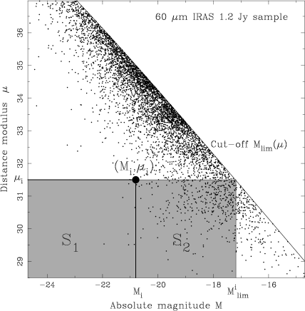
Figure 1: Distance modulus versus absolute magnitude for the 60 $\mu$m IRAS 1.2 Jy sample (5321 galaxies). The procedure for estimating the random variable $\zeta$ from Eq. (6) is illustrated.

The method described above is herein applied to the 60 $\mu$m IRAS 1.2 Jy sample (Fisher et al. 1995), a magnitude-redshift catalogue containing $5321$ galaxies and complete up to a flux $F_{60}=1.2$ Jy. Distance modulus and absolute magnitude are computed using $H_{0}=100$ km s^-1 Mpc^-1 for the value of the Hubble constant (the cut-off in apparent magnitude is expressed as $m_{\rm lim}=14.3187$ with this notation). The magnitudes have been k-corrected assuming a spectral slope $\alpha=-2$, implying that the maximum absolute magnitude introduced in Eq. (3) reads as $M_{\rm lim}(\mu)=m_{\rm lim}-{\rm k_{cor}}(\mu)-\mu$. The distribution of the sources in the $M$-$\mu$ plane is shown figure 1.

The peculiar velocity field model tested is the one-parameter predicted IRAS velocity field characterised by the parameter $\beta=\Omega_{0}^{0.6}/b_{I}$ (Strauss et al. 1992).

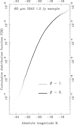
Figure 2: Reconstruction of the Cumulative Luminosity Function of the IRAS 1.2 Jy sources using the C^- method of Lynden-Bell (1971). The reconstructed CLF depends on the assumed velocity model.

3.1 Using apparent magnitude as the distance indicator

We have first applied the method using the apparent magnitude of IRAS galaxies as the distance indicator (restricting the analysis to the 4115 galaxies within the redshift range 1000-12000 km s^-1). The Cumulative Luminosity Function (CLF) $F(M)$ is presented in figure 2. Here the CLF has been reconstructed using the $C^{-}$ method of Lynden-Bell (1971) for two different velocity models, $\beta=0$ corresponding to the case where peculiar velocities are neglected and $\beta=1$. Note that the presence of peculiar velocities does not affect drastically the CLF reconstruction. The luminosity function of the IRAS galaxies does not exhibit any turnover towards the faint-end tail, at least within the observed range of magnitudes. This means that, because of the large dispersion of such a distance indicator and even if the number of galaxies is large, one cannot expect very strong constraints on the velocity model tested.

The correlation between the random variable $\zeta_{\beta}$ and the velocity modulus $u_{\beta}$ for $\beta=0.6$ is shown in figure 3. Variations of the coefficient of correlation as a function of the parameter $\beta$ are given in figure 4. This curve is a monotonic function, as expected. The preferred value of $\beta$ is the one corresponding to $\rho(\zeta_{\beta},u_{\beta})=0$ (here $\beta=0.1-0.15$).

Monte Carlo simulations have been used to calculate the discrepancy between $\rho(\zeta_{\beta},u_{\beta})$ and zero due to sampling fluctuations. Each simulation is a sample containing $N_{\rm gal}=4115$ galaxies with the same $\mu_{\beta}$ and $u_{\beta}$ as observed and for which the random variable $\zeta_{\beta}$ is computed following Eq. (6) where the rank $r_{i}$ is randomly generated according to a discrete uniform distribution between $1$ and $n_{i}$. The cumulative distribution function of $\rho(\zeta_{\beta},u_{\beta})$ obtained from a large number of simulations, under the null hypothesis that the true value of $\rho(\zeta_{\beta},u_{\beta})=0$, is shown in figure 5. Note that in practice this distribution does not depend on the amplitude of the quantity $u_{\beta}$ since the coefficient of correlation is a scale-free estimator of the correlation between two random variables.

The cumulative distribution function allows us to evaluate the probability that the observed $\rho$ is by chance greater than a given value, due to sampling fluctuations. A one-sided rejection test for the $\beta$ parameter can thus be constructed. For example, the models with $\beta\geq 0.7$ can be rejected with a confidence level of 95% and $\beta\geq 1.1$ with a confidence level of 99%. So our method applied to the IRAS sample, using the apparent magnitude of the galaxies as a distance indicator, permits already at this stage to reject high values for the parameter $\beta$.

Figure 3: Scatterplot indicating the correlation between the velocity modulus $u_{\beta}$ and the random variable $\zeta_{\beta}$ for $\beta=0.6$. A observed sample correlation coefficient of $\rho(\zeta_{\beta},u_{\beta})\simeq 0.02$ was found in this case.

Figure 4: The observed coefficient of correlation $\rho(\zeta_{\beta},u_{\beta})$ as a function of the parameter $\beta$. Confidence levels of rejection for the parameter $\beta$ are calculated from figure 5.

Figure 5: Cumulative distribution function of $\rho$ due to sampling fluctuations. This curve has been obtained by Monte Carlo simulations (see text).

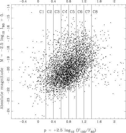
Figure 6: Observed correlation between the “colour index” $p=2.5\log_{10}(F_{100}/F_{60})$ and the absolute magnitude $M$. The sample has been subdivided into $8$ classes, $C_{i}$ according to the value of $p$.

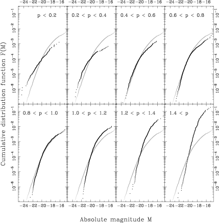
Figure 7: C^- reconstruction of the Cumulative Luminosity Function for the $8$ individual $C_{i}$ classes in $p$ (dark curves). The global CLF (i.e. no class) of figure 2 is shown for comparison (grey curve). The CLF’s have been arbitrarily normalised to $10^{-4}$ at $M=-20.$

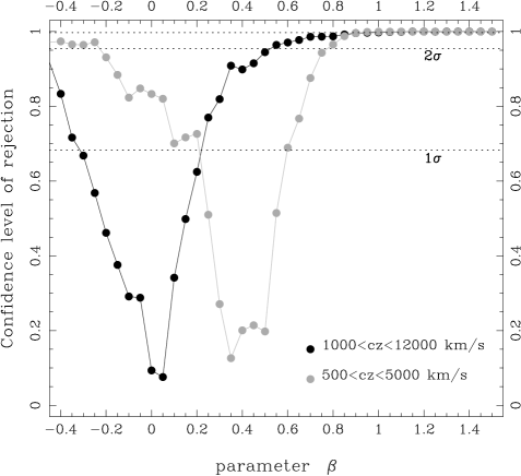
Figure 8: Confidence level of rejection for the parameter $\beta$ (see text).

Figure 9: Redshift distribution of the IRAS galaxies with $z\in[1000,12000]$ km s^-1 (4115 galaxies). The dark histogram represents this distribution when accounting for the natural weight $\propto 1/z$.

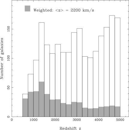
Figure 10: Redshift distribution of the IRAS galaxies with $z\in[500,5000]$ km s^-1 and galactic latitude $|b|>20$ (1621 galaxies). The grey histogram accounts for the natural weight $\propto 1/z$.

3.2 Introduction of a second parameter

In a second step, the analysis is refined by taking into account the observed correlation between the absolute magnitude $M$ and some “colour index” defined as $p=2.5\log_{10}(F_{100}/F_{60})$ (with $F_{100}$ the flux at 100 $\mu$m). The data have been grouped in $8$ classes by interval of $p$ (see figure 6). Because of the (weak) correlation between $p$ and $M$, the spread of the luminosity function for each of these classes taken individually is expected to be slightly smaller than the spread of the global luminosity function, and thus the accuracy of the distance indicator somewhat improved. Figure 7 illustrates such a trend.

For each individual class, the random variable $\zeta_{\beta}$ is computed according to Eq. (6). The correlation between $\zeta_{\beta}$ and the velocity modulus $u_{\beta}$ is after that evaluated for the whole sample. The influence of sampling fluctuations is estimated from Monte Carlo simulations, as described in the previous section. The results are presented in figure 8 in terms of the confidence level of rejection for the parameter $\beta$. More explicitly, the quantity plotted in ordinate is $1-2\,{\rm Prob}(\rho\leq-|\rho_{\rm obs}(\beta)|)$ where the probability that the coefficient of correlation $\rho$ is less than $-|\rho_{\rm obs}(\beta)|$ due to sampling fluctuations is given by the cumulative distribution function of $\rho$.

The method was first applied to the galaxies in the redshift range 1000-12000 km s^-1. It is found that $\beta\in[-0.35,0.25]$ at $1\sigma$, and that models with $\beta\geq 0.5$ can be rejected with a confidence level of 95%. This result is in disagreement with most of the analyses based on Tully-Fisher data e.g. VELMOD on MarkIII (Willick & Strauss 1998), ITF method on SFI (Da Costa et al. 1998), ROBUST method on MarkIII MAT sample (see next section), favouring a value of $\beta\simeq 0.5$. We interpret this discrepancy as follows.

When fitting a velocity model to data, the natural weight assigned by the fitting procedure to each galaxy is roughly proportional to the inverse of its redshift, because the accuracy of the distance indicator decreases as $1/z$. The mean effective depth of the volume where the velocity model is compared to data has to be estimated using these weights. For our first sample with $z\in[1000,12000]$ km s^-1, we find a mean effective depth of $3800$ km s^-1 (see figure 9).

In order to mimic the effective volume sampled by Tully-Fisher data we have applied the method to a truncated version of the IRAS sample containing 1621 galaxies with $z\in[500,5000]$ and galactic latitude $|b|>20$ (the mean effective depth of this sub-sample is now 2200 km s^-1, see figure 10). Figure 8 shows that the value of $\beta$ estimated from this truncated sample is fully consistent with the values obtained using Tully-Fisher data. An interpretation of these results could be that the predicted IRAS velocity field model, while successful in reproducing locally the cosmic flow, fails to describe the kinematics on larger scales.

However, as pointed out by our anonymous referee, the results derived above apply only to the extent that the photometry of the IRAS sample does not suffer from systematic errors. It is worthwhile to stress again that the philosophy of the ROBUST method is to impose very few assumptions – only that the luminosity function is independent of position, that the sample is strictly complete in apparent magnitude and that redshift and apparent magnitude measurements are not affected by systematic biases. Thus, our analysis could be affected if the IRAS photometry were (mildly) non-uniform. To evaluate the amplitude of such effects on our results would essentially require to adopt a realistic model for these systematic photometry variations. Since our primary goal here is to present a new method, we feel that such an error analysis is unwarranted. It is also worth noting that systematic errors in the IRAS photometry – if indeed present – would also affect methods for reconstructing the IRAS predicted peculiar velocity model. In particular, they would generate some systematic variations in the spatial selection function entering the weighting scheme used in density and velocity reconstruction (Strauss et al. 1992, Branchini et al. 1999), leading to systematic discrepancies between the IRAS predicted velocity field and the true cosmic flow. Moreover, it is interesting to note that the ROBUST method could easily be extended to provide a non-parametric test of the uniformity of photometry in redshift surveys; we will consider such an application in future work.

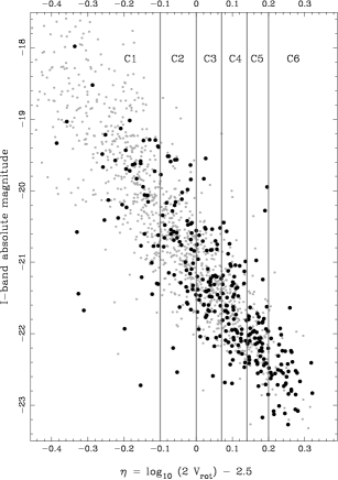
Figure 11: The Tully-Fisher relation for the MarkIII MAT sample (Willick et al. 1997b). A subsample of 318 galaxies (dark dots) complete in apparent magnitude up to $m_{\rm lim}=11.25$ mag. has been extracted. This subsample is divided in $6$ classes $C_{i}$ containing approximately $50$ galaxies each.

Figure 12: For each of the $6$ classes $C_{i}$, the $C^{-}$ reconstructed Cumulative Luminosity Function (dark dots). The solid curves are the expected cumulative distribution function of $M$ assuming a linear Direct (i.e. Forward) Tully-Fisher relation with Gaussian residuals and calibrated using the values proposed in Willick et al. (1998) (see text). For convenience in comparison, the $C^{-}$ reconstructed CLF’s $F_{\rm rec}(M)$ have been normalised such that $F_{\rm rec}(M_{i})=0.5$ at $M_{i}$ the mean absolute magnitude for each classes $C_{i}$ (dotted lines).

Figure 13: Confidence level of rejection for the parameter $\beta$ ($\beta=0.6\pm 0.125$).

Figure 14: Redshift distribution of the $318$ MarkIII MAT galaxies with $z\geq 500$ km s^-1 and apparent I-band magnitude $m\leq 11.25$ mag. The dark histogram takes into account the natural weight $\propto 1/z$.

4 Application to the MarkIII MAT sample

We have shown in the previous section that our method permits to extract valuable information on the cosmic velocity field by using the fluxes of the IRAS galaxies as a distance indicator. The potential of our method is illustrated in this section by treating a more classical case: the Tully-Fisher MarkIII MAT sample (Willick et al. 1997b and references therein).

In a first step we have selected from the 1355 galaxies of the MarkIII MAT catalog a subsample for which the selection effects in apparent magnitude are well described by a Heaviside cut-off, $\theta(m-m_{\rm lim})$. Assuming that the galaxies are homogeneously distributed in space, the value of $m_{\rm lim}$ can be found by analysing the variations in the logarithm of the cumulative count as a function of the limit in apparent magnitude – see for example figure 4 in Rauzy (1997). In a separate paper (Rauzy, in preparation) we propose anyway a simple tool for assessing the completeness in apparent magnitude of redshift-magnitude catalogues which does not require any assumption concerning the spatial distribution of the sources. This method is closely based on the statistical test presented in Efron & Petrosian (1992). We have applied this test to the MarkIII MAT sample, finding that the completeness in I-band corrected apparent magnitude is satisfied up to $m_{\rm lim}=11.25$ magnitudes.

Discarding, in addition, the galaxies with $z\leq 500$ km s^-1, we are left with a subsample containing $318$ galaxies. Note that the selection effects in redshift which affect the MarkIII MAT sample (Willick et al. 1996) are not a source of problems for our method. The Tully-Fisher relation for the $318$ extracted galaxies is shown in figure 11.

In a second step, we divided the subsample in $6$ classes $C_{i}$ according to the value of $\eta$, from the slower rotators in $C_{1}$ to the faster rotators in $C_{6}$ (see figure 11). The C^- reconstructed cumulative luminosity function is shown for each class in figure 12. If the binning in the log line-width parameter $\eta$ were narrow enough, one would expect the reconstructed luminosity function for the class $C_{i}$ to be centered on $M_{i}=a_{\rm DTF}\,\eta_{i}+b_{\rm DTF}$ and of dispersion $\sigma_{\rm DTF}(\eta_{i})$, where $\eta_{i}=<\eta>_{C_{i}}$ denotes the mean of the $\eta$’s in $C_{i}$ and $a_{\rm DTF}$, $b_{\rm DTF}$ and $\sigma_{\rm DTF}(\eta_{i})$ are respectively the slope, zero-point and dispersion of the Direct (i.e. Forward) Tully-Fisher relation. We plot in figure 12 the expected culmulative luminosity function when a linear DTF relation with gaussian residuals is assumed and using the values proposed in Willick et al. (1998) for the calibration parameters. The width of the bins has been accounted for by adding in quadrature to the dispersion $\sigma_{\rm DTF}(\eta_{i})$ the product of $|a_{\rm DTF}|$ and the standard deviation of the $\eta$’s in each class $C_{i}$ . For convenience in comparison, Each C^- reconstructed CLF $F_{\rm rec}(M)$ has been normalised such that $F_{\rm rec}(M_{i})=0.5$.

It is not clear from figure 12 whether a linear DTF relation with gaussian residuals is plainly successful in reproducing the data. Note in particular that the C^- reconstructed CLF’s for the slow rotators do not exhibit a turnover towards the faint magnitudes. To question the validity of a linear Tully-Fisher relation is anyway beyond the scope of the present paper. At this stage it is however worthwhile to mention that our method makes a very conservative use of Tully-Fisher information. In fact, we require to assume neither a linear TF relation nor a gaussian distribution for its residuals.

The result of the ROBUST method applied to the MarkIII MAT catalog is shown in figure 13. The analysis was performed as described in section 3.2. The mean effective depth of the subsample is 2100 km s^-1 (see figure 14). We find a value of $\beta=0.6\pm 0.125$, in complete agreement with the VELMOD and ITF method applied to similar Tully-Fisher data (Willick et al. 1997a and 1998, Davis et al. 1996, Da Costa et al. 1998).

We want however to emphasise the robustness of our approach compared to these two fitting methods. Firstly, no assumptions have been made herein concerning the linearity of the Tully-Fisher law, as is required by both the VELMOD and the ITF method. Secondly, we do not need the sample to be free of selection effects in the log line-width parameter $\eta$ as is the case for the ITF method. Thirdly, the spatial distribution of the sources, the selection effects in redshift and the shape of the distribution function of the TF residuals need not be specified, as is required by the maximum likelihood VELMOD method.

5 Conclusion

We presented a method for fitting peculiar velocity models to complete flux limited magnitude-redshift catalogues, using the luminosity function of the sources as a distance indicator, i.e. assuming that the distribution function of the absolute magnitudes of the galaxies does not depend on the spatial position.

Our method is based on a null-correlation approach. For a given peculiar velocity field model parametrised by a parameter $\beta$, we defined a random variable $\zeta_{\beta}$, computable from the observed redshifts and apparent magnitudes of the sampled galaxies, which has the property of being statistically independent on the position in space (and thus on the modelled radial peculiar velocities themselves) if and only if the parameter $\beta$ matches its true value $\beta^{\star}$. Therefore any test of independence between the random variable $\zeta_{\beta}$ and the modelled velocities or similar quantities provides us with an unbiased estimate of the value of $\beta^{\star}$. The method can be easily generalised to velocity models parametrised by an $N$-dimensional vector ${\bf\beta}=(\beta_{1},\beta_{2},...,\beta_{N})$.

The method is characterised by its robustness. No assumptions are made concerning the spatial distribution of sources and their luminosity function and selection effects in redshifts are also allowed. The required strict completeness in apparent magnitude can moreover be checked independently (Rauzy, in preparation). Furthermore the inclusion of additional observables correlated with the absolute magnitude is straightforward.

The predicted IRAS peculiar velocity model characterised by the density parameter $\beta$ has been tested on two samples, the Tully-Fisher MarkIII MAT sample and the 60 $\mu$m IRAS 1.2 Jy sample using the fluxes as the distance indicator.

The application of our method to the MarkIII MAT sample gives a value of $\beta=0.6\pm 0.125$, in excellent agreement with the results obtained previously by the VELMOD and ITF methods on similar datasets. Our method is however more robust than these two fitting methods. In particular, we make a very conservative use of the Tully-Fisher information. We do not require to assume the linearity of the Tully-Fisher relation nor a gaussian distribution of its residuals.

We showed that our method allows to extract some valuable informations on the peculiar velocity field from the fluxes of the IRAS 1.2 Jy sample. The poor accuracy of the distance indicator (due to the broad spread of the luminosity function) is balanced in this case thanks to the large number of galaxies contained in the sample. The IRAS sample permits to probe the cosmic flow at larger scales. Indeed, the mean effective depth of the volume in which the velocity model is compared to the data is almost twice the mean effective depth of the MarkIII MAT sample.

The application of our method to an IRAS subsample truncated in distance, of an effective depth similar to the MarkIII MAT sample, gives a value of $\beta$ in accord with the values obtained using Tully-Fisher data. On the other hand when the application is performed on the whole sample, we found that the predicted IRAS velocity models with $\beta\geq 0.5$ can be rejected with a confidence level of $95\%$. These results suggest that the predicted IRAS velocity model, while successful in reproducing locally the cosmic flow, fails to describe the kinematics on larger scales.

Note that these results do not lead to dismiss the linear “biasing” paradigm. As the errors on the predicted IRAS velocity field increase with distances, it could be that the predictions at the scales considered herein, i.e. beyond $5000$ km s^-1, drastically differ from the true cosmic flow (see for example Davis et al. 1995).

References

- [1989] Bertschinger E., Dekel A., 1989, ApJ, 336, L5
- [1990] Bertschinger E., Dekel A., Faber S. M., Burstein D., 1990, ApJ, 364, 370
- [1999] Branchini E., Teodoro L., Frenck C. S., Schmoldt I., Efstathiou G., White S. D. M., Saunders W., Sutherland W., Rowan-Robinson M., Keeble O., Tadros H., Maddox S., Oliver S. 1999, MNRAS 308, 1
- [1992] Bicknell G. V., 1992, ApJ, 399, 1
- [1991] Bigot G., Triay R., Rauzy S., 1991, Phys. Lett. A, 158, 282
- [1995] Choloniewski J., 1995, MNRAS, 275, L79
- [1999] Colless M., Burstein D., Davies R. L., McMahan R. K., Saglia R. P., Wegner G., 1999, MNRAS, 303, 813
- [1993] Courteau S., Faber S. M., Dressler A. Willick J. A., 1993, ApJ, 412, L51
- [1999] Courteau S., Willick J. A., Strauss M. A., Schlegel D. S., Postman M., 1999, ASP Conf. Series, Eds Courteau, Strauss & Willick, in press
- [1998] da Costa L. N., Nusser A., Freudling W., Giovanelli R., Haynes M. P., Salzer J. J., Wegner G., 1998, MNRAS, 229, 425
- [1999] Dale D. A., Giovanelli R., Haynes M. P., Campusano L. E., Hardy E., Borgani S., 1999, ApJ, 510, 11
- [1996] Davis M., Nusser A., Willick J. A., 1996, ApJ, 473, 22
- [1990] Dekel A., Bertschinger E., Faber S. M., 1990, ApJ, 364, 349
- [1994] Dekel A., 1994, ARA&A, 32, 371
- [1999] Dekel A., Eldar A., Kolatt T., Yahil A., Willick J. A., Faber S. M., Courteau S., Burstein D., 1999, ApJ, 522, 1
- [1992] Efron B., Petrosian V., 1992, ApJ, 399, 345
- [1996] Ekholm T., 1996, A&A, 308, 7
- [1995] Fisher K. B.,Huchra J. P., Strauss M. A., Davis M., Yahil A., Schlegel D., 1995, ApJS, 100, 69
- [1978] Fliche H-H., Souriau J-M., 1979, A&A, 78, 87
- [1995] Freudling W., Da Costa L. N., Wegner G., Giovanelli R., Haynes M. P., Salzer J. J., 1995, AJ, 110, 920
- [1997] Giovanelli R., Haynes M. P., Herter T., Vogt N. P., Wegner G., Salzer J. J., Da Costa L. N., Freudling W., 1997a, AJ, 113, 22
- [1997] Giovanelli R., Haynes M. P., Herter T., Vogt N. P., Da Costa L. N., Freudling W., Salzer J. J., Wegner G., 1997b, AJ, 113, 53
- [1998] Giovanelli R., Haynes M. P., Freudling W., Da Costa L. N., Salzer J. J. Wegner G., 1998, ApJ, 505, 91
- [1992] Han M., Mould J. R., 1992, ApJ, 396, 453
- [1990] Hendry M. A., Simmons J. F. L., 1990, A&A, 237, 275
- [1994] Hendry M. A., Simmons J. F. L., 1994, ApJ, 435, 515
- [1999] Hudson M. J., Smith R. J., Lucey J. R., Schlegel D. J., Davies R. L., 1999, ApJ, 512, 79
- [1992] Landy S. D., Szalay A., 1992, ApJ, 391, 494
- [1994] Lauer T.R., Postman M., 1994, ApJ, 425, 418
- [1971] Lynden-Bell D., 1971, MNRAS, 155, 95
- [1988] Lynden-Bell D., Dressler A., Burstein D., Davies R. L., Faber S. M., Terlevich R. J., Wegner G., 1988, ApJ, 326, 19
- [1992] Mathewson D. S., Ford V. L., Buchhorn M., 1992, ApJS, 81, 413
- [1995] Newsam A. M., Simmons J. F. L., Hendry M. A., 1995, A&A, 294, 627
- [1995] Nusser A., Davis M., 1995, MNRAS, 276, 1391
- [1993] Rauzy S., Lachièze-Rey M., Henriksen R. N., 1993, A&A, 273, 357
- [1995] Rauzy S., Lachièze-Rey M., Henriksen R. N., 1995, Inverse Problems, 11, 765
- [1996] Rauzy S., Triay R., 1996, A&A, 307, 726
- [1997] Rauzy S., 1997, A&AS, 125, 255
- [1997] Riess A. G., Davis M., Baker J., Kirshner R. P., 1997, ApJ, 488, 1
- [1994] Sandage A., 1994, ApJ, 430, 13
- [1998] Sigad Y., Eldar A., Dekel A., Strauss M. A., Yahil A., 1998, ApJ, 495, 516
- [1992] Strauss M. A., Davis M., Yahil A.,Huchra J. P., 1992, ApJ, 385, 421
- [1999] Strauss M. A., 1999, ASP Conf. Series, Eds Courteau, Strauss & Willick, in press
- [1997] Theureau G., Hanski M., Teerikorpi P., Bottinelli L., Ekholm T., Gouguenheim L., Paturel G., 1997, A&A, 319, 435
- [1997] Theureau G., Hanski M., Ekholm T., Bottinelli L., Gouguenheim L., Paturel G., Teerikorpi P., 1997, A&A, 322, 730
- [1998] Theureau G., Rauzy S., Bottinelli L., Gouguenheim L., 1998, A&A, 340, 21
- [1990] Teerikorpi P., 1990, A&A, 234, 1
- [1999] Teerikorpi P., Ekholm T., Hanski M., Theureau G., 1999, A&A, 343, 713
- [1997] Tonry J. L., Blakeslee J. P., Ajhar E. A., Dressler A., 1997, ApJ, 475, 399
- [1994] Triay R., Lachièze-Rey M., Rauzy S., 1994, A&A, 289, 19
- [1996] Triay R., Rauzy S., Lachièze-Rey M., 1996, A&A, 309, 1
- [1999] Wegner G., Colless M., Saglia P. P., McMahan R. K., Davies R. L., burstein D., Baggley G., 1999, MNRAS, 305, 259
- [1990] Willick J. A., 1990, ApJ, 351, L5
- [1994] Willick J. A., 1994, ApJS, 92, 1
- [1995] Willick J. A., Courteau S., Faber S. M., Burstein D., Dekel A., 1995, ApJ, 446, 12
- [1996] Willick J. A., Courteau S., Faber S. M., Burstein D., Dekel A., Kolatt T., 1996, ApJ, 457, 460
- [1997] Willick J. A., Strauss M. A.,Dekel A., Kolatt T., 1997a, ApJ, 486, 629
- [1997] Willick J. A., Courteau S., Faber S. M., Burstein D., Dekel A., Strauss M. A., 1997b, ApJS, 109, 333
- [1998] Willick J. A., Strauss M. A., 1998, ApJ, 507, 64
- [1999] Willick J. A. 1999a, ApJ, 516, 47
- [1999] Willick J. A., 1999b, ASP Conf. Series, Eds Courteau, Strauss & Willick, in press