Multiparameter estimation with the Pseudo-$C_{l}$ method

We apply the Pseudo-$C_{l}$ formalism to obtain an unbiased, approximate method for efficient simultaneous estimation of several cosmological parameters from large, almost full–sky cosmic microwave background data sets.

1 Introduction

Within the standard model of cosmology there are about 10 parameters which characterise the properties of our Universe. It is one of the key goals of future CMB experiments such as MAP and Planck to determine these cosmological parameters to high precision. This undertaking faces the challenge that realistic CMB data is necessarily incomplete and noisy. The Galaxy obscures roughly a third of the sky and because of the smallness of the anisotropy signal, detector noise is not negligible in the analysis. This leads to the computational challenge which was expertly described at this meeting in the contribution by Borrill$\!{}^{{\bf?}}$.

In this talk we apply the pseudo-$C_{l}$ formalism$\!{}^{{\bf?}}$ to this problem and show that it can be used to develop an approximate form of the likelihood which has several useful properties: it is Gaussian and hence easy to apply; it does not suffer from the usual disadvantages of Gaussian approximations such as obtaining negative estimates of positive definite quantities; it is computationally efficient with memory usage of $N_{pix}$ and number of operations scaling as $N_{pix}^{\frac{3}{2}}$ per likelihood evaluation with a very small pre–factor leading to thousands of likelihood evaluations per CPU hour.

2 The approximation scheme

Given a true CMB sky T and an experimental setup and observation strategy (encoded in the beam pattern B, the survey geometry $W$ and the noise distribution on the sky $W_{N}T_{N}$) we can represent the observed temperature anisotropy map as

$$\tilde{T}({\bf\gamma})=W({{\bf{\gamma}}})\left[B\ast T({{\bf{\gamma}}})+W_{N}({{\bf{\gamma}}})T_{N}({{\bf{\gamma}}})\right]$$ (1)

This temperature field $\tilde{T}$ can be decomposed into spherical harmonics coefficients

$$\tilde{a}_{lm}=\int_{{\cal O}}d\Omega\>Y^{\ast}_{lm}({{\bf{\gamma}}})\tilde{T}({{\bf{\gamma}}}).$$ (2)

The notation “$\int_{\cal O}$” denotes integration over the fraction of the sky covered by the survey. These combine into the observed power spectrum coefficients which we call pseudo-$C_{l}$,

$$\tilde{C}_{l}=\frac{1}{2l+1}\sum_{m}\left|{\tilde{a}_{lm}}\right|^{2}.$$ (3)

In $\!{}^{{\bf?}}$ we derive the exact statistics of the pseudo-$C_{l}$, under the assumptions of azimuthal survey geometry and noise which is uncorrelated from pixel to pixel and whose amplitude varies only from latitude to latitude. The results we derived were still a superb approximation for strongly non-azimuthal noise patterns.

We found that in the case of large sky coverage the Pseudo-$C_{l}$ distributions were nearly indistinguishable from Gaussian distributions of the same means and variances as long as $l>100$. The fact that many of the cosmological parameters are sensitive to the power spectrum at precisely these small scales led us to propose the following approximation to the likelihood:

$$\widehat{\cal L}(C_{l})=\prod_{l>100}\exp\left[-\frac{\left(C_{l}-\left\langle{\tilde{C_{l}}}\right\rangle\right)^{2}}{\left\langle{\Delta\tilde{C}_{l}^{2}}\right\rangle}\right]$$ (4)

In this approximation, maximum likelihood estimation has reduced to simple $\chi^{2}$ fitting, however with the correct means and variances.

To illustrate, we solve the problem of estimating 3 parameters ($\Omega_{c}$ $\Omega_{b}$ and $H_{0}$) simultaneously from a sky with $12\times 10^{6}$ pixels of which $66\%$ are observed. The response of the experiment is modelled as a Gaussian beam of FWHM 12 arcminutes. The noise template is inhomogeneous and not azimuthally symmetric with rms amplitude of $124\mu K$ per 3.5 arcminute pixel. To compare with the naive Gaussian approach and to show that our method is unbiased, we compute maximum (approximate) likelihood estimates from 100 realisations of the sky and plot a representation of the empirical distribution of parameter estimates in three dimensions in Figures 1 (naive $\chi^{2}$) and 2 (our approach).

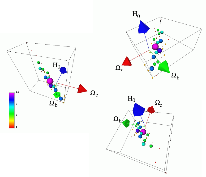
Figure 1: Multi–parameter estimation of $\Omega_{0}$, $\Omega_{b}$ and $H_{0}$ using naive $\chi^{2}$ fitting. The three panels show three views from different directions of the empirical distribution of the parameter estimates. Each sphere represents one bin of the three–dimensional distribution. The size and shading of a sphere indicates the number of realisations (out of 100 total) which led to parameter estimates within its bin. The true parameter values are at the origin of the coordinate axes. It is clearly visible that the distribution is shifted with respect to the true distribution by an amount which is inconsistent with the width of the distribution. In other words the true values could be ruled out at high significance if this estimate was used.

Our estimates are unbiased. The distributions of the estimates are clearly centered on the true values.

We stress that our approach avoids the usual difficulties of Gaussian approximations. For example, even though we use the Gaussian pdf, which of course does not exclude negative $C_{l}$, they are assigned an exceedingly small probability. This is because no attempt is made to subtract out the noise contribution from the pseudo–$C_{l}$ — instead it is modelled consistently and the (signal$\times$noise) cross term which is present in each realisation is not allowed to dominate.

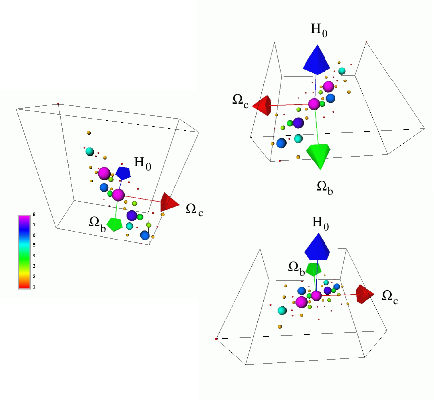
Figure 2: Multi–parameter estimation of $\Omega_{0}$, $\Omega_{b}$ and $H_{0}$ using our approximate likelihood Eq. (4). The three panels show three views from different directions of the empirical distribution of the parameter estimates. Each sphere represents one bin of the three–dimensional distribution. The size and shading of a sphere indicates the number of realisations (out of 100 total) which led to parameter estimates within its bin. The true parameter values are at the origin of the coordinate axes. It is clearly visible that the distribution is correctly centered on the true values.

References

References

- [1] J. Borrill 2000, in these proceedings
- [2] B. D. Wandelt, E. F. Hivon, and K. M. Górski. 2000, submitted to Physical Review D.