The Chandra X-Ray Observatory’s Radiation Environment and the AP-8/AE-8 Model

Abstract

The Chandra X-ray Observatory (CXO) was launched on July 23, 1999 and reached its final orbit on August 7, 1999. The CXO is in a highly elliptical orbit, approximately 140,000 km x 10,000 km, and has a period of approximately 63.5 hours ($\approx$ 2.65 days). It transits the Earth’s Van Allen belts once per orbit during which no science observations can be performed due to the high radiation environment. The Chandra X-ray Observatory Center (CXC) currently uses the National Space Science Data Center’s “near Earth” AP-8/AE-8 radiation belt model to predict the start and end times of passage through the radiation belts. However, our scheduling software uses only a simple dipole model of the Earth’s magnetic field. The resulting B, L magnetic coordinates, do not always give sufficiently accurate predictions of the start and end times of transit of the Van Allen belts. We show this by comparing to the data from Chandra’s on-board radiation monitor, the EPHIN (Electron, Proton, Helium Instrument particle detector) instrument. We present evidence that demonstrates this mis-timing of the outer electron radiation belt as well as data that also demonstrate the significant variablity of one radiation belt transit to the next as experienced by the CXO. We also present an explanation for why the dipole implementation of the AP-8/AE-8 model is not ideally suited for the CXO. Lastly, we provide a brief discussion of our on-going efforts to identify a model that accounts for radiation belt variability, geometry, and one that can be used for observation scheduling purposes.

Keywords: Chandra, space missions, radiation environment, radiation belts, radiation models, radiation damage, magnetosphere

1 INTRODUCTION

Just past midnight on July 23, 1999, the space shuttle Columbia lifted-off from Cape Canaveral, Florida. In its payload bay lay the Chandra X-ray Observatory (CXO), the primary cargo of the STS-93 mission. Just under 8 hours after launch, Chandra was deployed from the space shuttle. However, it would be nearly two weeks later, after an Inertial Upper Stage booster and several “burns” by its own propulsion system, that Chandra would reach its final orbit. The CXO is now the third of NASA’s “great observatories” in space.

The CXO’s operational orbit has an apogee of approximately 140,000 km and a perigee of nearly 10,000 km, with a $28.5^{\circ}$ initial inclination. The CXO’s highly elliptical orbit, with an orbital period of approximately 2.65 days, results in high efficiency for observing. Moreover, the fraction of the sky occulted by the Earth is small over most of the orbital period, as is the fraction of time when the detector backgrounds are high as the flight system dips into the Earth’s radiation belts. Consequently, approximately 85% of Chandra’s orbit is available for observing. In fact, uninterrupted observations lasting as long as 2.3 days are possible[1].

The CXO carries two focal plane science instruments: the High Resolution Camera (HRC) and the Advanced CCD Imaging Spectrometer (ACIS). The Observatory also possesses two objective transmission gratings: a Low Energy Transmission Grating (LETG) that is to be primarily used with the HRC, and the High Energy Transmission Grating (HETG) that is to be primarily used with the ACIS. In addition to these instruments, Chandra also carries a radiation monitor – the Electron, Proton, Helium Instrument (EPHIN) particle detector.

In order to attain this high level of observing efficiency, a robust radiation environment model is required so that times of high radiation are known a priori when producing a weekly sequence of CXO observations. The CXO orbit encounters higher radiation levels as the spacecraft approaches perigee. Routine science observing will cease whenever the scheduling system has indicated that the maximum radiation levels are excessive.

These times of high radiation are required not only so that observations do not take place but also so as to not cause significant radiation damage to the CXO’s focal plane instruments over the expected on-orbit design life. To that end, the Chandra X-ray Center (CXO) currently uses the National Space Science Data Center’s (NSSDC) “near Earth” AP-8/AE-8 radiation belt model to predict the start and end times of passage through the radiation belts.

In this paper, we provide a brief synopsis of the CXO and its instruments in Section 2. In Section 3, we present an overview of the Earth’s magnetosphere and the EPHIN detector. The AP-8/AE-8 model is described in Section 4. The following section, Section 5, presents our evidence that our implementation of the AP-8/AE-8 model does not always give sufficiently accurate predictions of the start and end times of transit of the Earth’s Van Allen belts. In that same section, we present an explanation for why the dipole implementation of the AP-8/AE-8 model gives inaccurate start and end times for radiation belt transit 75% of the time (for low energy electrons). Lastly, in Section 6, we provide a brief summary of our current operating procedure and the on-going work being done by the CXC and NASA’s Marshall Space Flight Center’s Radiation Environment working group in identifying a new radiation model to be used for scheduling purposes.

2 CHANDRA X-RAY OBSERVATORY’S FOCAL PLANE INSTRUMENTS

The observatory consists of a spacecraft system and a telescope/science-instrument payload. The spacecraft system provides mechanical controls, thermal control, electric power, communication/command/data management, and pointing and aspect determination. This section, however, only briefly describes the two focal plane instruments on-board the CXO, the HRC and the ACIS, since the main emphasis in this paper is the Observatory’s radiation environment and not the instruments per se. Nevertheless, the AXAF Observatory Guide[2] and the AXAF Science Instrument Notebook[3] contain a wealth of information about the CXO and its instruments. More in depth discussions of the Chandra mission, spacecraft, other instruments and subsystems are presented elsewhere. [4]^, [5]^, [6]^, [7]

2.1 High Resolution Camera (HRC)

The High Resolution Camera, HRC, is a microchannel plate (MCP) instrument. It is comprised of two detector elements, a $\sim$ 100 mm square optimized for imaging (HRC-I) and a $\sim$ 20 x 300 mm rectangular device optimized for the Low Energy Transmission Grating (LETG) Spectrometer readout (HRC-S).

The HRC has the highest spatial resolution imaging on Chandra – $\leq$ 0.5 arcsec (FWHM) – matching the High Resolution Mirror Assembly (HRMA) point spread function most closely. The HRC energy range extends to low energies, where the HRMA effective area is the greatest. HRC-I has a large field of view (31 arcmin on a side) and is useful for imaging extended objects such as galaxies, supernova remnants, and clusters of galaxies as well as resolving sources in a crowded field. The HRC has good time resolution (16 $\mu$sec), valuable for the analysis of bursts, pulsars, and other time-variable phenomena and limited energy discrimination, E/$\Delta$E $\sim$ 1 ($<$ 1 keV). The HRC-S is used primarily for readout of the low-energy grating, LETG, for which its large format with many pixels gives high spectral resolution ($>$ 1000, 40-60 $\AA$) and wide spectral coverage (3 - 160 $\AA$).

2.2 Advanced CCD Imaging Spectrometer (ACIS)

ACIS is the Advanced CCD Imaging Spectrometer. It is comprised of two arrays of CCDs, one optimized for imaging wide fields (2x2 chip array; ACIS-I), the other optimized for grating spectroscopy and for imaging narrow fields (1x6 chip array; ACIS-S). Each array is shaped to follow the relevant focal surface. In conjunction with the HRMA, the ACIS imaging array provides simultaneous time-resolved imaging and spectroscopy in the energy range $\sim$ 0.5 - 10.0 keV. When used in conjunction with the High Energy Transmission Gratings (HETG), the ACIS spectroscopic array will acquire high resolution (up to E/$\Delta$E = 1000) spectra of point sources[8]. The CCDs have an intrinsic energy resolution (E/$\Delta$E) which varies from $\sim$5 to $\sim$50 across the energy range.

ACIS employs two varieties of CCD chips. Most of the chips are “front-side” (or FI) illuminated. That is, the front-side gate structures are facing the incident X-ray beam from the HRMA. Two of the 10 chips (S1 and S3) have had treatments applied to the back-sides of the chips, removing the insensitive, undepleted, bulk silicon material and leaving only the photo-sensitive depletion region exposed. These “back-side”, or BI chips, are deployed with the back side facing the HRMA. BI chips have a substantial improvement in low-energy quantum efficiency as compared to the FI chips because no X-rays are lost to the insensitive gate structures but suffer from poorer charge transfer inefficiency, poorer spectral resolution, and poorer calibration accuracy. In addition, early analysis from on-orbit data indicate that the BIs are more susceptible to “background flares”, which may compromise a measurement, than are FIs[9]. These background flares (i.e. rapid increases in detector background) are thought to be a consequence of Chandra’s radiation environment.

3 THE EARTH’S MAGNETOSPHERE AND THE EPHIN DETECTOR

Before describing the EPHIN detector, we will first provide a brief overview of the Earth’s magnetosphere.

3.1 The Earth’s Magnetosphere

The solar wind, a streaming ionized plasma, flows at all times and in all directions from the Sun. When it encounters a magnetized obstacle, the Earth for example, a magnetosphere is formed (see Figure  1). The magnetosphere of a planet is defined as the region where the particle motion is determined by the magnetic field of the planet[10]. The magnetopause is the boundary layer which separates this region from the solar wind plasma. At the bow shock, the solar wind, when sensing the obstacle prior to reaching the magnetopause, undergoes an abrupt transition from supersonic flow to subsonic flow. This shock allows the wind to be slowed, heated, and deflected around the planet in the magnetosheath. The polar cusps of clefts are singular points at northern and southern polar latitudes where the magnetic field is zero. Only here can solar wind particles directly reach the top of the atmosphere. Field lines in the neighbourhood are either closed toward the dayside or open toward the nightside, where the magnetotail is formed. The dayside extension of the magnetosphere varies between 4.5 and 20 $R_{Earth}$ depending on the solar wind pressure, whereas the nightside extension reaches several hundred $R_{Earth}$, much farther than the orbit of the Moon. The plasmasphere is a region of high density ($\sim$ $10^{3}$ $cm^{-3}$), cold ($\sim$ 1 eV) plasma, an extension of the ionosphere to altitudes up to 3-4 $R_{Earth}$.

The region in which science observations must not occur is in the Van Allen belts. The radiation belts, or the Van Allen belts, consist of particles in orbits that circle the Earth from about 1,000 km above the surface to a geocentric distance of $\sim$ 6 $R_{Earth}$. Contrary to particles in the plasmasphere, these particles are trapped at high energies. These particles enter the radiation belts through a variety of means, including radial diffusion from more distant regions with accompanying acceleration, and the decay of neutrons from the sputtering of the atmosphere by galactic cosmic rays. Whereas energetic protons form a single belt, as illustrated in the top panel of Figure  2, electrons form two belts – an inner and an outer belt (as illustrated in the bottom panel). A co-ordinate system with L (L designates the magnetic-drift shell and is equal to the distance in $R_{Earth}$ from the center of the Earth to the point where the field line crosses the equator) and B, the magnetic field, organizes the radiation belt data quite well[10].

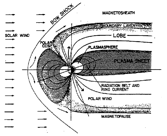
Figure 1: Structure of the magnetosphere (Crooker and Siscoe, 1986)[11]

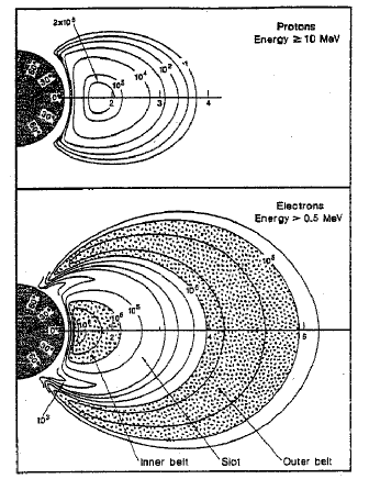
Figure 2: Earth’s Radiation Belts. The top panel shows the contours of the omnidirectional flux (counts/($cm^{2}$ s)) of protons with energies greater than 10 MeV. The bottom panel shows the contours of the omnidirectional flux of electrons with energies greater than 0.5 MeV. (Kivelson and Russell, 1995)[12]

3.2 The EPHIN Detector

The natural space environment can cause a range of problems for a spacecraft and may even compromise its mission. Environmental factors include the radiation belts, solar energetic particles, cosmic rays, plasma, gases, and micrometeorites. In this paper, we will only address the radiation belts.

The CXO radiation environment is monitored by the EPHIN detector (although the HRC anti-coincidence shield may also be used to some degree). The EPHIN was designed and manufactured as a scientific instrument for the Solar and Heliospheric Observatory and the Chandra X-ray Observatory by the University of Kiel. A detailed description of the EPHIN instrument can be found in Müller-Mellin et al. (1995)[13] and Sierks (1997)[14].

Briefly, the EPHIN consists of an array of 5 silicon detectors with anti-coincidence to measure the energy of electrons in the range 150 keV - 10 MeV, and hydrogen/helium isotopes in the energy range 5 - 53 MeV/nucleon. Please see Table  1 for a more precise overview of EPHIN’s scientific data channels. As Figure  3 illustrates, the field of view of EPHIN is $\sim$ 83 degrees. The stack of 5 silicon detectors operates in a multi-dE/dx vs. E mode and it is surrounded by an anti-coincidence shield (Figure  3). Two passivated ion-implanted silicon detectors (PIPS) A and B define the 83 degree field of view with a geometric factor of 5.1 $cm^{2}$ sr. The silicon detectors are divided into 6 segments. This coarse position sensing permits sufficient correction for path length variations needed to resolve isotopes of hydrogen and helium. The directional information cannot be used for anisotropy measurements as particles from different directions are summed when they have the same degree of oblique incidence. Another important advantage of this sector paradigm is the capability to implement a commandable or self-adaptive geometric factor [15]. This permits measurements of fluxes as high as 2 x $10^{5}$ counts/($cm^{2}$ s sr) without significant dead time losses. A third benefit is the reduction in capacitance at the input to the charge sensitive pre-amplifiers, resulting in low-noise performance.

Lastly, the lithium-drifted silicon detectors (Si(Li)) C, D, and E stop electrons up to 10 MeV and hydrogen and helium nuclei up to 53 MeV/n. The ion-implanted detector F will allow particles stopping in the telescope to be distinguished from penetrating particles. The fast plastic scintillation detector G, viewed by a 1-inch photomultiplier and used in anti-coincidence, is indispensible for accurate electron measurements. This whole stack of detectors is mounted in an aluminum housing, the aperature being covered by a 2 $\mu$m thin titanium foil for light tightness. A second foil in the viewing cone is made of 76 $\mu$m aluminized Kapton (original specifications in Figure  3 called for 8 $\mu$m) for thermal control[15].

Table 1: EPHIN Energy Ranges[10]

EPHIN Channel	Energy Range	Energy Width
	[MeV] or [MeV/n]	[MeV] or [MeV/n]
E150	0.25 - 0.70	0.45
E300	0.67 - 3.00	2.3
E1300	2.64 - 6.18	3.6
E3000	4.80 - 10.4	5.6
P4	5.0 - 8.3	3.3
P8	8.3 - 25.0	16.7
P25	25.0 - 41.0	16.0
P41	41.0 - 53.0	12.0
H4	5.0 - 8.3	3.3
H8	8.3 - 25.0	16.7
H25	25.0 - 41.0	16.0
H41	41.0 - 53.0	12.0
INT	e: $>$ 8.7
	p,h: $>$ 53

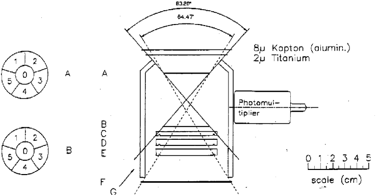
Figure 3: EPHIN sensor schematics with detector A and B segmentation pattern on the left. The geometric factor varies with penetration depth (solid lines: view cone for particles stopping in B, dashed lines: view cone for penetrating particles). [15]

4 AP/AE TRAPPED PARTICLE RADIATION MODEL

The CXO’s orbital parameters were designed to minimise the time spent in the Van Allen radiation belts. Energetic particles contribute to the background rate and can damage the CCD detectors over time. Hence, the apogee is $\sim$ 140,000 km. Now, the time spent above 60,000 km is a good indicator of the time spent outside the radiation belts, however in order to maximize orbital efficiency, a robust radiation environment model is required; the AP-8/AE-8 radiation belt model is the one the CXC has implemented to accomplish this task. The primary outputs from the AE-8/AP-8 model are the spatial fluxes of trapped electrons and protons in the near Earth environment.

These maps contain omnidirectional, integral electron (AE maps) and proton (AP maps) fluxes in the energy range 0.04 MeV to 7 MeV for electrons and 0.1 MeV to 400 MeV for protons in the Earth’s radiation belt (L = 1.2 to 11 for electrons, L = 1.17 to 7 for protons)[16]. The fluxes are stored as functions of energy, L-value, and B/$B_{0}$ (magnetic field strength normalized to its equatorial value on the field line). These maps are based on data from more than 20 satellites that operated from the early sixties to the mid-seventies. Indeed, the data contained within these flux maps span 14 years (1966 to 1980). The AE-8/AP-8 model is the latest edition in a series of updates starting with AE-1 and AP-1 in 1966[16].

The different previous electron models can be characterised as inner (L = 1.2-3) or outer (L = 3-11) zone models and as models for solar cycle maximum or minimum conditions. However, AE-8 is the first model that covers the whole L range and both solar cycle extrema. The AP maps differ in energy range and solar cycle phase. AP-8 is the first model for the whole energy range and both solar cycle extrema[16].

However, one significant shortcoming of the AP-8/AE-8 model is that none of the flux maps consider time variations beyond the solar cycle minimum/maximum distinction. A study carried out by the NSSDC[17] found that for the inner zone electrons, the two dominant time effects are caused by magnetic storms and the solar cycle. In particular, magnetic storms strongly affect electrons with energies higher than 0.7 MeV at higher L-shells, whereas the solar cycle effect is most significant for electrons with energies below 0.7 MeV. It is important to note that magnetic storm effects are still not yet included in any of the AE maps. It is thought that the largest errors occur where steep gradients in spatial and spectral distribution exist and where time variations are not well understood[16]. Therefore, it is clear that one has to be careful in extrapolating these models to later epochs.

The electron AE-8 and proton AP-8 flux maps for solar maximum and minimum are available through the NSSDC as part of its “RADBELT 1988” software program (see http://nssdc.gsfc.nasa.gov/). The software provides omnidirectional, integral (or differential) electron or proton fluxes in the Earth’s radiation belt by using an interpolation procedure that uses the AE-8 and AP-8 trapped particle flux maps. It is the output from this software program that we compare against EPHIN data in the next section.

5 AP-8/AE-8 MODEL VS. EPHIN DATA

In order to make a meaningful comparison of the AP-8/AE-8 model with the EPHIN data, the correct information must be provided to the radiation belt software program. Since EPHIN possesses 4 electron channels and 4 proton channels (see Table  1), the NSSDC software routine was queried to find the start times when various specified thresholds would be exceeded, and the end times when flux predictions would be below the same thresholds for each EPHIN channel. These time spans are then, effectively, a proxy for radiation belt transit (as measured by the EPHIN).

Now, the offline scheduling system (OFLS), which incorporates the radiation belt software that the CXC uses to produce transit predictions, is not designed to search for specific ranges of energies for flux excursions. That is, it can only do single energies with multiple flux values; a single time is generated at each entry and exit where the flux and energy conditions are met. Below is a sample query that was used to determine start and end times of radiation belt transit.

FOR EPHIN ELECTRONS:

E150: Flux = 1 cts/s/$cm^{2}$/sr Energy $\geq$ 0.25 MeV

E300: Flux = 1 cts/s/$cm^{2}$/sr Energy $\geq$ 0.67 MeV

E1300: Flux = 1 cts/s/$cm^{2}$/sr Energy $\geq$ 2.64 MeV

E3000: Flux = 1 cts/s/$cm^{2}$/sr Energy $\geq$ 4.80 MeV

FOR EPHIN PROTONS:

P4: Flux = 4.93 cts/s/$cm^{2}$/sr Energy $\geq$ 5.0 MeV

P8: Flux = 1 cts/s/$cm^{2}$/sr Energy $\geq$ 8.3 MeV

P25: Flux = 1 cts/s/$cm^{2}$/sr Energy $\geq$ 25.0 MeV

P41: Flux = 1 cts/s/$cm^{2}$/sr Energy $\geq$ 41.0 MeV

The time spans (i.e., entries and exits) for which the above conditions were met have been determined since Day 200 of 1999 to the middle of February, 2000. The time spans, which corresponds to an EPHIN proton or electron channel, have been superimposed on the EPHIN data. Generally, the agreement between the radiation belt model and the EPHIN data is quite poor. For instance, of the 73 radiation belt transits seen in the EPHIN E150 channel, 55 were poorly timed ($\sim$ 75%). That is, of the 73 radiation belt transits investigated, nearly 75% showed EPHIN exceedances of the flux criteria specified above before the expected exceedance from the AE-8/AP-8 model. Similar numbers for the E300, E1300, and E3000 channels are 48 (66%), 20 (27%) and 20 (27%), respectively.

Three of the most extreme examples of these radiation belt mis-timing are presented in Figures  4,  5, and  6. Although similar data exists for the EPHIN proton channels, they are not included in this paper since it appears that in a high electron flux environment, electrons can mimic a proton signal in the low energy EPHIN proton channels. More work is needed to fully understand and solve this problem before that data is presented.

These plots also demonstrate the significant variability in radiation belt transits, however, one has to be very careful in drawing conclusions about temporal variability during radiation belt transits based on these plots alone since the EPHIN detector saturates during perigee transit. The effect of the EPHIN anti-coincidence counter, when in saturation, will distort the electron fluxes and time profile in the innermost part of the radiation belts, approximately when E150 rates exceed $10^{5}counts/s/cm^{2}/sr$. The indicated intensities in Figures  4,  5, and  6 during these intervals, should be regarded as lower limits only. An internal CXC memo, however, used EPHIN’s leakage currents as a probe to understand Chandra’s radiation environment and also found significant variablity in radiation belt intensity and duration[18]. In the following table, we note the average value of the discrepancy (between model and data) for each EPHIN channel for the three perigee transits presented in Figures  4,  5, and  6.

Table 2: Average Time Differences Between EPHIN Electron Channels and the OFLS

EPHIN Channel	$|T_{EPHIN}$-$T_{OFLS}$$|_{entry}$	$|T_{EPHIN}$-$T_{OFLS}$$|_{exit}$
	ks	ks
E150	9.1	10.0
E300	10.0	10.0
E1300	4.3	2.4
E3000	3.4	3.4

Hence, we observe that the predictive value of the AP-8/AE-8 model is adequate, though certainly not optimal. In particular, the mis-timing of the softer species is seen to be worse than that for their harder counterparts. Since the degradation of the ACIS FI CCDs is believed to be due to protons in the range $\sim$ 100 kev - $\sim$ 400 keV, it is important for us to accurately predict the location of these relatively low-energy species. Due to their low energy, however, these species are also very dynamic, and can rapidly change their spatial extent subject to the day-to-day solar conditions. In contrast, the implementation of AP-8/AE-8 model used is a static one and can only take into account solar MAX vs. MIN conditions, and we believe this is the major source of the scheduling error of the radiation belts we witness, especially for low-energy species. Other models, such as a 3-D version of the Magnetospheric Specification and Forecast Model[19] currently under development will be better able to take into account solar variations on a day-to-day (or week-to-week) basis and will thus increase Chandra’s observing efficiency by reducing the necessary “padding” of the scheduled radiation belts which is currently implemented (discussed in Section  6) as a CXC mission planning policy.

Figure 4: AE-8 radiation belt model predictions against EPHIN data on Day 355. Note AE-8 predictions are based on an integral above an energy threshold (specified within the text) whereas the EPHIN electron channel has a much narrower energy window.

Figure 5: AE-8 radiation belt model predictions against EPHIN data on Day 371. Note AE-8 predictions are based on an integral above an energy threshold (specified within the text) whereas the EPHIN electron channel has a much narrower energy window.

Figure 6: AE-8 radiation belt model predictions against EPHIN data on Day 379. Note AE-8 predictions are based on an integral above an energy threshold (specified within the text) whereas the EPHIN electron channel has a much narrower energy window.

6 CXC OPERATING PROCEDURE AND FUTURE WORK

Although the ACIS hardware is fairly robust with respect to radiation, repeated exposure to high levels of radiation will gradually degrade the hardware (see ACIS Flight Software User’s Guide). In fact, shortly after opening the telescope door to celestial sources for the first time, it was found that the FI ACIS CCDs had suffered radiation damage (http://chandra.harvard.edu). This radiation damage is believed to have been caused by forward scattering of protons with energies between 100 keV and 400 keV, associated with the radiation belts, from Chandra’s mirrors during passage through the Van Allen belts. Since this discovery, a number of policy changes have been implemented that will hopefully prevent further radiation damage from occuring.

Because of this mis-timing of the radiation belts by our scheduling software, we have had to be more conservative in identifying times we shut down the ACIS for the radiation belt transit and times we turn on the ACIS post-perigee transit. From Table  2, it can be seen that if a 10-11 ks “pad” was added to both sides of the predicted radiation belt times, one would get better agreement with the EPHIN data. Indeed, a more thorough analysis of Chandra’s radiation history to date yielded the same result. Therefore, it was decided to pad the AE-8 predictions of radiation belt entry and exit by 13 ks. This is because the AE-8 radiation belt transit time span is longer than the AP-8 time span since the proton belt lies below the outer electron belt (see Figure 2). Thus, this choice leads to the more conservative approach.

Additionally, since it is believed to be protons focused on the ACIS as it sat in the focal plane during a series of radiation belt transits early in the mission that has caused most of the radiation damage (and not this mis-timing of the “wings” of the radiation belt itself), it was also decided to place the HRC in the focal plane (i.e., keep ACIS out from the focal plane) during subsequent radiation belt transits and to have it partially close its door to protect its instrumentation. This translation of the science instruments occurs at the “modified” start and end times of radiation belt transit.

To protect ACIS during the science operations portion of the orbit, new threshold levels were uplinked to the CXO. Now, EPHIN data is monitored by Chandra’s on-board computer (OBC) which will activate commands to safe the focal plane instruments during periods of high radiation (e.g. a solar flare or coronal mass ejection). All of these new policy changes and our monitoring scheme will be discussed in more depth in a forthcoming paper[20].

However, clearly all of the above policies are “short-term” solutions. What is really needed is a more robust, higher fidelity radiation belt model that provides reliable start and end times of radiation belt transit. To that end, work is currently in progress to produce an empirical model of the Earth’s radiation belt that will provide the CXC with reliable perigee transit information[21].

Lastly, because of the present radiation damage that has been sustained by our FI ACIS CCDs, our radiation monitor, EPHIN, has become of paramount importance in preserving the health and safety of the CXO. Thus, work has been on-going to further analyse its data, to better understand the saturation issues with perigee transit, and to develop a procedure that is able to account for electron contamination of the proton data. Clearly, more work is needed so that the outstanding science being returned by the Chandra X-ray Observatory can continue unattenuated for many more years to come.

References

- [1] S. L. O’Dell and M. C. Weisskopf, “Advanced X-ray Astrophysics Facility (AXAF): Calibration Overview,” in X-Ray Optics, Instruments, and Missions, R. B. Hoover and A. B. W. II, eds., Proc. SPIE 3444, pp. 2–18, 1998.
- [2] A. T. 403, AXAF Observatory Guide, Chandra X-ray Science Center, Cambridge, MA, 1997.
- [3] A. T. 401, AXAF Science Instrument Notebook, Chandra X-ray Science Center, Cambridge, MA, 1995.
- [4] M. C. Weisskopf, S. L. O’Dell, and R. F. Elsner, “Advanced X-ray Astrophysics Facility - AXAF an Overview,” in X-Ray and Extreme Ultraviolet Optics, R. B. Hoover and A. B. W. II, eds., Proc. SPIE 2515, 1995.
- [5] M. V. Zombeck, “Advanced X-ray Astrophysics Facility AXAF,” in Proceedings of the International School of Space Science Course on X-Ray Astronomy, Aquila, Italy CfA Preprint 403, 1996.
- [6] T. H. Markert, C. R. Canizares, D. Dewey, M. McGuirk, C. S. Pak, and M. L. Schattenburg, “High Energy Transmission Grating Spectrometer (HETGS) for AXAF,” in EUV, X-Ray, and Gamma-Ray Instrumentation for Astronomy V, Proc. SPIE 2280, 1994.
- [7] A. C. Brinkman, J. J. van Rooijen, J. A. M. Bleeker, J. H. Dijkstra, J. Heise, P. A. J. de Korte, R. Mewe, and F. Paerels, “Low Energy X-ray Transmission Grating Spectrometer for AXAF,” Astro. Lett. 26, p. 73B, 1987.
- [8] A. T. 402, AXAF Proposers’ Guide, Chandra X-ray Science Center, Cambridge, MA, 1997.
- [9] P. P. Plucinsky and S. N. Virani, “Observed On-Orbit Background of the ACIS Detector on the Chandra X-ray Observatory,” in X-Ray Optics, Instruments, and Missions, J. Truemper and B. Aschenbach, eds., Proc. SPIE 4012, p. (this volume), 2000.
- [10] R. Mueller-Mellin, EPHIN Response to the AXAF Radiation Environment, Doc. No. EPH-RRE-001, Kiel, Germany, 1997.
- [11] N. U. Crooker and G. L. Siscoe, “The Effect of the Solar Wind on the Terrestrial Environment,” in Physics of the Sun, P. Sturrock, T. Holzer, D. Mihalas, and R. Ulrich, eds., vol. III, 1986.
- [12] M. Kivelson and C. Russell, Introduction to Space Physics, Cambridge University Press, Cambridge, England, 1995.
- [13] R. Mueller-Mellin, H. Kunow, V. Fleissner, E. Pehlke, E. Rode, N. Roschmann, C. Scharmberg, H. Sierks, P. Rusznyak, I. E. S. McKenna-Lawlor, J. Sequeiros, D. Meziat, S. Sanchez, J. Medina, L. der Peral, M. Witte, R. Marsden, and J.Henrion, “Costep - comprehensive suprathermal and energetic particle analyser,” Solar Physics 162, pp. 483–504, 1995.
- [14] H. Sierks, Kosmische Teilchen im Sonnensystem - Messung Geladener Teilchen mit dem Kieler Instrument EPHIN an Bord der SOHO-Raumsonade, Ph.D. Thesis, University of Kiel, 1997.
- [15] R. Mueller-Mellin, H. Sierks, H. Kunow, E. Pehlke, V. Fleissner, E. Rode, and C. Scharmberg, “Calibration of the Electron Proton Helium Instrument (EPHIN) Aboard the AXAF-I Spacecraft,”
- [16] J. I. Vette, “AE/AP Trapped Particle Flux Maps 1966-1980,” in NSSDC Space Models Web Page, http://nssdc.gsfc.nasa.gov/space/model/magnetos/aeap.html, ed., 1996.
- [17] M. Teague and J. Vette, “The Inner Zone Electron Model AE-5,” National Space Science Data Center NSSDC 72-10, 1972.
- [18] S. N. Virani, P. P. Plucinsky, and R. Mueller-Mellin, “Using EPHIN’s Detector Leakage Current To Understand Radiation Belt Transits,” in CXC Internal Memo, http://asc.harvard.edu/acis/radbelt, ed., 1999.
- [19] J. Freeman, R. Wolf, R. Spiro, B. Hausman, B. Bales, D. Brown, K. Costello, R. Hilmer, R. Lambour, A. Nagai, and J. Bishop, “The Magnetospheric Specification and Forecast Model,” preprint , 1995.
- [20] S. L. O’Dell, M. Bautz, W. Blackwell, , D. Brautigam, Y. Butt, R. Cameron, B. Dichter, R. Elsner, S. Gussenhoven, J. Kolodziejczak, J. Minow, D. Swartz, A. Tennant, S. N. Virani, and K. Warren, “in preparation,” Proc. SPIE , 2000.
- [21] W. Blackwell, J. Minow, and S. N. Virani, “in preparation,” Proc. SPIE , 2000.