On the oxygen abundance determination in HII regions

Abstract

The problem of the line intensities – oxygen abundance calibration has been considered. We confirm the idea of McGaugh (1991) that the strong oxygen lines ($[OII]\lambda\lambda 3727,3729$ and $[OIII]\lambda\lambda 4959,5007$) contain the necessary information for determination of accurate abundances in low-metallicity (and may be also in high-metallicity) HII regions. It has been found that the excitation parameters $p_{3}$ or $p_{2}$ (which are defined here as contributions of the radiation in $[OIII]\lambda\lambda 4959,5007$ lines and in $[OII]\lambda\lambda 3727,3729$ lines to the ”total” oxygen radiation respectively) allow to take into account the variations in $R_{23}$ values among HII regions with a given oxygen abundance. Based on this fact a new way of the oxygen abundance determination in HII regions (p – method) has been constructed and corresponding relations between $[OII]\lambda\lambda 3727,3729$, $[OIII]\lambda\lambda 4959,5007$ line intensities and the oxygen abundance have been derived empirically using the available oxygen abundances determined via measurement of temperature-sensitive line ratios ($T_{e}$ – method).

In parallel a new $R_{23}$ calibration has been derived on the base of recent data and compared to previous calibrations. For oxygen-rich HII regions the present $R_{23}$ calibration is close to that of Edmunds and Pagel (1984): their calibration has the same slope but is shifted towards higher oxygen abundances by around 0.07 dex as compared to the present calibration.

1 Introduction

The oxygen abundance is one of the fundamental characteristics of a galaxy. The radial distribution of the oxygen abundance in a galaxy (together with radial distributions of gas and star surface mass densities) provides a strong constraint on models of (chemical) evolution. In the general case the intensities of oxygen emission lines in spectra of HII regions depend not only on the oxygen abundance but also on physical conditions. The oxygen abundance can be derived from accurate measurement of temperature-sensitive line ratios, such as $[OIII]\lambda\lambda 4959,5007/\lambda 4363$. This method will be referred to as the $T_{e}$ – method.

Unfortunately, in oxygen–rich HII regions the temperature-sensitive lines like $[OIII]\lambda 4363$ are too weak to be detected. For such HII regions empirical abundance indicators based on more readily observable lines were suggested (Pagel et al 1979, Alloin et al 1979). The empirical oxygen abundance indicator $R_{23}=(I_{[OII]\lambda 3727,\lambda 3729}+I_{[OIII]\lambda 4959,\lambda 5007})/I_{H\beta}$ suggested by Pagel et al (1979) has found widespread acceptance and use for the oxygen abundance determination in HII regions where the temperature-sensitive lines are undetectable. This method will be referred to as the $R_{23}$ – method. Several workers have suggested calibrations of $R_{23}$ in terms of oxygen abundance (Edmunds & Pagel 1984, McCall & Rybski and Shields 1985, Dopita & Evans 1986, Zaritsky & Kennicutt and Huchra 1994, among others). Zaritsky et al’s calibration is an average of the three former calibrations.

The oxygen abundances of HII regions in many irregular galaxies are derived with the $T_{e}$ – method. Those in HII regions of the Milky Way have also been determined with the $T_{e}$ – method (Shaver et al 1983). This data is a base for many investigations of chemical evolution of our Galaxy. Oxygen abundances in HII regions of many spiral galaxies have been derived with the $R_{23}$ – method. As indicated by Skillman et al (1996), the precise choice of the O/H – $R_{23}$ calibration is not critical in differential comparisons of the abundance properties of different objects if the oxygen abundances in all the objects are derived with the same O/H – $R_{23}$ calibration. However, the comparison of the abundance properties of galaxies where the oxygen abundances were determined with the $T_{e}$ – method (irregular galaxies, Milky Way and a few other spiral galaxies) and galaxies where the oxygen abundances were determined with the $R_{23}$ – method (spiral galaxies) is justified only if the two methods agree. The existing O/H – $R_{23}$ calibrations (Edmunds & Pagel 1984, McCall & Rybski and Shields 1985, Dopita & Evans 1986, McGaugh 1991) are based on then-available oxygen abundance determinations through the $T_{e}$ – method and HII region models, whereas more oxygen abundance determinations through the $T_{e}$ – method are available now. Then the existing O/H – $R_{23}$ calibrations should be verified in the light of more recent data and a new calibration derived if necessary.

The search for a line intensities – O/H calibration which results in the same oxygen abundances as the $T_{e}$ – method is the goal of this study. The line intensities – O/H calibration has been derived in Section 2. A discussion will be presented in Section 3. Section 4 is a brief summary.

2 Line intensities – O/H calibration

In order to check whether the $T_{e}$ – method and the $R_{23}$ – method result in the same oxygen abundances the $X_{23}$( = log $R_{23}$) versus 12 + logO/H diagram for the Milky Way Galaxy HII regions from Shaver et al (1983) and HII regions in spiral and irregular galaxies together with O/H – $R_{23}$ calibrations after Edmunds & Pagel 1984, McCall et al 1985, Dopita & Evans 1986, and Zaritsky et al 1994 has been constructed, Fig.1. The data for HII regions in irregular galaxies were taken from (Izotov and Thuan 1998, 1999: Izotov, Thuan, and Lipovetsky 1994, 1997; Kobulnicky and Skillman 1996, 1997, 1998: Kobulnicky et al 1997; Skillman et al 1994;Thuan, Izotov, and Lipovetsky 1995; Vilchez and Iglesias-Paramo 1998). The data for HII regions in spiral galaxies were taken from (Esteban et al 1998; Esteban et al 1999a,b; Garnett et al 1999; Gonzalez-Delgado et al 1995; Kwitter and Aller 1981; Pagel, Edmunds, and Smith 1980; Peimbert, Torres-Peimbert, and Dufour 1993; Shaver et al 1983; Shields and Searle 1978; van Zee et al 1998; Vilchez and Esteban 1996; Vilchez et al 1988; Webster and Smith 1983). These lists (involving 151 data points) do not pretend to be exhaustive ones. In the case of low-metallicity HII regions there is a large set of data with recent high-quality determinations of oxygen abundance with the $T_{e}$ – method, therefore earlier ones were not included in our list. In the case of high-metallicity HII regions there are a few recent high-quality determinations of the oxygen abundance with the $T_{e}$ – method, therefore we have to include in our list all available oxygen abundance determinations although some data were obtained around 20 years ago. In a few cases there are two independent determinations of the oxygen abundance in the same object or independent determinations in different parts of the HII region. Since the goal of the present study is a search for the line intensities – oxygen abundance relation but not an investigation of the chemical properties of individual galaxies, the independent determinations of oxygen abundance in the same object were included in the list as individual data points. Our data confirm the conclusion of Kennicutt et al (2000) that the Edmunds and Pagel calibration (Edmunds & Pagel 1984) provides a more robust diagnostic of oxygen abundance, but an inspection of the Fig.1 shows that it still results in an oxygen abundance that is higher than the mean at any given log$R_{23}$. Thus, none of the existing $R_{23}$ – O/H calibration can reproduce the available data well enough and a new one should be constructed.

Figure 1: The OH – log$R_{23}$ diagram. The positions of HII regions in spiral galaxies (circles) (the HII regions in our Galaxy from Shaver et al 1983 (S83) are indicated by plusses) and in irregular galaxies (triangles) are shown together with OH – $R_{23}$ calibrations of different authors: Edmunds & Pagel 1984 (EP), McCall et al 1985 (MRS), Dopita & Evans 1986 (DE), and Zaritsky et al 1994 (ZKH).

Figure 2: The $p_{2}$ versus $X_{2}$ diagram for HII regions in spiral and irregular galaxies (points). The positions of HII regions with 7.1 $\leq$ 12+log(O/H)_Te $\leq$ 7.3 are shown by circles, HII regions with 7.4 $\leq$ 12+log(O/H)_Te $\leq$ 7.6 are shown by triangles, HII regions with 8.0 $\leq$ 12+log(O/H)_Te $\leq$ 8.1 are shown by plusses. Solid lines are best fits to positions of HII regions with 7.1 $\leq$ 12+log(O/H)_Te $\leq$ 7.3 and HII regions with 7.4 $\leq$ 12+log(O/H)_Te $\leq$ 7.6. Dashed lines are lines with slope equal to 1.

Figure 3: The $p_{3}$ versus $X_{3}$ diagram for HII regions in spiral and irregular galaxies (points). The positions of HII regions with 7.1 $\leq$ 12+log(O/H)_Te $\leq$ 7.3 are shown by circles, HII regions with 7.4 $\leq$ 12+log(O/H)_Te $\leq$ 7.6 are shown by triangles, HII regions with 8.0 $\leq$ 12+log(O/H)_Te $\leq$ 8.1 are shown by plusses. Solid lines are best fits to positions of HII regions with 7.1 $\leq$ 12+log(O/H)_Te $\leq$ 7.3, HII regions with 7.4 $\leq$ 12+log(O/H)_Te $\leq$ 7.6, and HII regions with 8.0 $\leq$ 12+log(O/H)_Te $\leq$ 8.1. Dashed lines are lines with slope equal to 1.

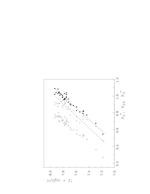
Figure 4: The oxygen abundances (O/H)_Te versus observed X₂₃ and computed X${}_{2}^{*}$ and X${}_{3}^{*}$ values for selected subset of galaxies with best defined oxygen abundances. The O/H versus $X^{*}_{2}$ diagram is presented by triangles, the O/H versus $X^{*}_{3}$ diagram is presented by points, and the O/H versus $X_{23}$ diagram is presented by plusses The solid line is the best fit to the O/H versus $X^{*}_{3}$ relation, the dashed line is the best fit to the O/H versus $X_{23}$ relation.

Figure 5: The differences between oxygen abundances derived with the suggested p – method and derived with the $T_{e}$ – method (circles) and differences between oxygen abundances derived with the $R_{23}$ – method and derived with the $T_{e}$ – method (crosses) for selected subset of HII regions in irregular galaxies with best determined oxygen abundances (O/H)_Te.

Figure 6: The differences between oxygen abundances derived with the suggested p – method and derived with the $T_{e}$ – method (circles) and differences between oxygen abundances derived with the $R_{23}$ – method and derived with the $T_{e}$ – method (plusses) as a function of parameter $p_{3}$ for selected subset of HII regions in irregular galaxies with best determined oxygen abundances through the ${Te}$ – method. The solid line is the best fit $\Delta log(O/H)_{P_{3}}$ – $p_{3}$ relation, the dashed line is the best fit $\Delta log(O/H)_{R_{23}}$ – $p_{3}$ relation.

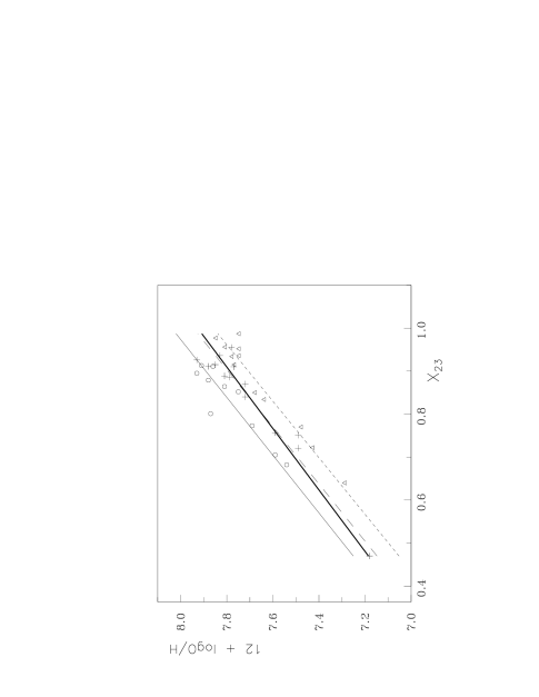
Figure 7: The oxygen abundances (O/H)_Te versus X₂₃ diagram for selected subset of galaxies with best defined oxygen abundances. The HII regions with $p_{3}$ $<$ –0.1 are shown by circles (and corresponding best fit is presented by the thin solid line), the HII regions with –0.05 $>$ $p_{3}$ $>$ –0.1 are shown by plusses (and corresponding best fit is presented by the long-dashed line), the HII regions with $p_{3}$ $>$ –0.05 are shown by triangles (and corresponding best fit is presented by the short-dashed line). The thick solid line is the general best fit, i.e. best fit to all data (the same as in Fig.4).

Figure 8: The oxygen abundances (O/H)_Te versus observed X₂₃ (plusses) and computed X${}_{2}^{*}$ (triangles) and X${}_{3}^{*}$ (circles) values for total set of HII regions in spiral and irregular galaxies. The solid line is the adopted O/H – $X_{2}^{*}$ relation, the dashed line is the adopted O/H – $X_{23}$ relation.

Figure 9: The differences between oxygen abundances derived with the suggested p – method and derived with the $T_{e}$ – method (triangles) and differences between oxygen abundances derived with the $R_{23}$ – method and derived with the $T_{e}$ – method (plusses) as a function of parameter $p_{2}$. The solid line is the best fit $\Delta log(O/H)_{P_{2}}$ – $p_{2}$ relation, the dashed line is the best fit $\Delta log(O/H)_{R_{23}}$ – $p_{2}$ relation.

Figure 10: The upper branch (12+logO/H $>$ 8.15) of the X₂₃ – O/H diagram. The oxygen abundances derived with the $T_{e}$ – method (original data from literature) are shown by circles, the abundances derived with the suggested p – method are shown by plusses. The solid line is the O/H – $R_{23}$ calibration obtained here, the dashed line is the O/H – $R_{23}$ calibration from Edmunds and Pagel (1984).

Figure 11: The radial distributions of the oxygen abundance in NGC2403 derived by Garnett et al (1997) with the $T_{e}$ – method (circles), derived with the p – method (plusses), and derived with Edmunds and Pagel calibration ($R_{23}$ – method).

The simplest way to construct the line intensities – O/H relation is a traditional approach: to find a best fit $R_{23}$ – O/H relation using available HII regions in which oxygen abundances were determined with the $T_{e}$ – method. A one-to-one correpondence between the oxygen abundance and the R₂₃ value is implied in this approach, i.e. the variations in $R_{23}$ values among HII regions with a given oxygen abundance are not taken into consideration. However, McGaugh (1991) pointed out that the geometrical factor is important in low-metallicity HII regions and $R_{23}$ must be supplemented with additional information. This can be verified in the following simple way. Let us consider the $X_{2}$ versus $p_{2}$ and $X_{3}$ versus $p_{3}$ diagrams, Figs.2, 3. (The following notations will be accepted here: $R_{2}$ = $I_{[OII]\lambda 3727+\lambda 3729}/I_{H\beta}$, $X_{2}$ = log$R_{2}$, $R_{3}$ = $I_{[OIII]\lambda 4959+\lambda 5007}/I_{H\beta}$, $X_{3}$ = log$R_{3}$, $R_{23}$ =$R_{2}$ + $R_{3}$, $X_{23}$ = log$R_{23}$, $p_{2}$ = $X_{2}$ - $X_{23}$, and $p_{3}$ = $X_{3}$ - $X_{23}$.) If the value of $R_{23}$ is constant for HII regions with similar oxygen abundances, then the HII regions with similar oxygen abundances should lie along a straight line with a slope equal to 1 in the $X_{2}$ versus $p_{2}$ and $X_{3}$ versus $p_{3}$ diagrams. The positions of HII regions with oxygen abundances logO/H+12 in the range from 7.1 to 7.3 are shown by circles, in the range interval from 7.4 to 7.6 are shown by triangles, and in the range interval from 8.0 to 8.1 are shown by plusses, Figs.2, 3. The linear best fits to corresponding data are presented by solid lines. Dashed lines are lines with a slope equal to 1. Inspection of Figs.2, 3 shows that the HII regions with similar oxygen abundances lie indeed along a straight line, but a slope of this straight line is not equal to 1.

The fact that the slope of the best fit differs from 1 has far-reaching implications: it means that value of $logR_{23}$ varies systematically with $p_{3}$ and a quantity other than $logR_{23}$ should be used in oxygen abundance determination. In order to verify the reality of this fact and to clearly recognize the consequences, the subset of selected HII regions with best determined oxygen abundances through the $T_{e}$ – method has been considered. This subset includes the low-metallicity (12+logO/H $<$ 7.95) HII regions from Izotov & Thuan (1998, 1999) and Izotov & Thuan, and Lipovetsky (1994, 1997). Since the HII regions with similar oxygen abundances lie along a straight line with a slope other than unity the extrapolated intersect $X_{3}$ is not equal to $R_{23}$. The notation X${}^{*}_{3}$ will denote the value of $X_{3}$ extrapolated to p₃ = 0. Similarly, the notation X${}^{*}_{2}$ will be adopted for the value of $X_{2}$ extrapolated to p₂ = 0. The data for the selected subset of HII regions result in the following relation between $\Delta X_{3}$ = X${}_{3}^{obs}$ – X${}^{*}_{3}$ and $\Delta$p₃

$$\Delta X_{3}=2.20\;\Delta p_{3}=2.20\;p_{3},$$ (1)

where $\Delta p_{3}$ = p₃ by virtue of $p^{*}_{3}$ = 0 was adopted. The corresponding relation between $\Delta X_{2}$ = X${}_{2}^{obs}$ – X${}^{*}_{2}$ and $\Delta$p₂ = p₂ is given by equation

$$\Delta X_{2}=0.76\;\Delta p_{2}=0.76\;p_{2}.$$ (2)

Using these equations the values of X${}^{*}_{3}$ and X${}^{*}_{2}$ have been computed for all the HII regions from the selected subset.

The oxygen abundances (O/H)_Te versus observed X₂₃ and versus computed X${}_{2}^{*}$ and X${}_{3}^{*}$ values for the selected subset of HII regions are shown in Fig.4. The O/H versus $X^{*}_{2}$ diagram is presented by triangles, the O/H versus $X^{*}_{3}$ diagram is presented by points, and the O/H versus $X_{23}$ diagram is presented by plusses The solid line is the best fit to the O/H versus $X^{*}_{3}$ relation, the dashed line is the best fit to the O/H versus $X_{23}$ relation. The X₂₃ values are positioned between corresponding X${}^{*}_{2}$ and X${}^{*}_{3}$ values. Since $p_{3}$ values are more close to zero than $p_{2}$ values the extrapolated intersect $X_{3}$ seem to be more reliable than $X_{2}$. Inspection of Fig.4 shows that linear approximations are acceptable for the relations between O/H and X₂₃ and between O/H and X${}^{*}_{3}$. Thus, the values of X₂₃ and X${}^{*}_{3}$ have been calibrated in terms of oxygen abundance using the linear approximation. The best fits to the data result in the following relations (Fig.4)

$$12+log(O/H)_{R_{23}}=6.53+1.40\;X_{23},$$ (3)

$$12+log(O/H)_{P_{3}}=6.35+1.45\;X^{*}_{3}.$$ (4)

Using these equations two values of the oxygen abundance $(O/H)_{R_{23}}$ and $(O/H)_{P_{3}}$ have been obtained for every HII region in the selected subset. The determination of the oxygen abundance through $p_{3}$ (or $p_{2}$) will be referred to as the p – method.

The differences $\Delta log(O/H)_{R_{23}}$ between oxygen abundances $(O/H)_{R_{23}}$ derived with the $R_{23}$ – method and oxygen abundances $(O/H)_{Te}$ derived with the $T_{e}$ – method are shown in Fig.5 by plusses as a function of $(O/H)_{Te}$. The differences $\Delta log(O/H)_{P_{3}}$ = $(O/H)_{P_{3}}$ - $(O/H)_{Te}$ are are shown in Fig.5 by circles. It can be seen in Fig.5 that the mean value of $\Delta log(O/H)_{P_{3}}$ is appreciable lower ($\sim$ 0.042 dex) than the mean value of $\Delta log(O/H)_{R_{23}}$ ($\sim$ 0.086 dex).

The differences $\Delta log(O/H)_{P_{3}}$ and $\Delta log(O/H)_{R_{23}}$ as a function of p₃ are shown in Fig.6. As seen in Fig.6 the error in the value of the oxygen abundance derived with the $R_{23}$ – method involves two parts: the first part is a random error comparable to the random error in the p – method, and the second part is a systematic error. The origin of this systematic error is as follows. In a general case the intensities of oxygen emission lines in spectra of HII regions depend not only on the oxygen abundance but also on the physical conditions (hardness of the ionizing radiation and geometrical factor). Then in the determination of the oxygen abundance from line intensities the physical conditions in the HII region should be taken into account. In the $T_{e}$ – method this is done via $T_{e}$. In the p – method, physical conditions are allowed for via parameter p, i.e. the parameter p can be considered as some kind analogy of the electron temperature $T_{e}$ in the oxygen abundance determination. In the $R_{23}$ – method the physical conditions in HII region are ignored. Therefore, the oxygen abundances derived with the $T_{e}$ – method and with the p – method involve only random errors (this is a strong argument that the physical conditions in HII region are well taken into account via parameter p), while the oxygen abundances derived with the $R_{23}$ – method involve a systematic error caused by the failure to take into account the differences in physical conditions in different HII regions.

The fact that the value of $logR_{23}$ in HII regions with a given oxygen abundance varies systematically with $p_{3}$ can be directly established from detailed consideration of the $X_{23}$ versus O/H diagram, Fig.7. The HII regions with $p_{3}$ $<$ –0.1 are shown by circles (and corresponding best fit is presented by the thin solid line) in Fig.7, the HII regions with –0.05 $>$ $p_{3}$ $>$ –0.1 are shown by plusses (and corresponding best fit is presented by the long-dashed line), the HII regions with $p_{3}$ $>$ –0.05 are shown by triangles (and corresponding best fit is presented by the short-dashed line). The thick solid line in Fig.7 is the general best fit, i.e. the best fit to all data (the same as in Fig.4). Inspection of Fig.7 shows that the HII regions with different values of $p_{3}$ lie along different straight lines shifted relative to each other depending on the value of $p_{3}$. According to the model grid of McGaugh (1991) this shifting is accounted for by the variations in the geometrical factors. The general best fit O/H – X₂₃ (equation (3)) is very close to the best fit to the data for HII regions with –0.05 $>$ $p_{3}$ $>$ –0.1, Fig.7. The HII regions with $p_{3}$ $>$ –0.05 are shifted to the right from the general best fit and as a consequence the $(O/H)_{R_{23}}$ values derived in these HII regions with equation (3) are higher than $(O/H)_{Te}$, Fig.6. Conversely, the HII regions with $p_{3}$ $<$ –0.10 are shifted to the left from the general best fit in Fig.7, and so the $(O/H)_{R_{23}}$ derived for them from equation (3) are lower than $(O/H)_{Te}$, Fig.6.

Thus, the above discussion of the subset of selected HII regions with best determined oxygen abundances through the $T_{e}$ – method suggests that i) the oxygen abundances derived with the $R_{23}$ – method involve a systematic error caused by the failure to take into account the differences in physical conditions in different HII regions, ii) the physical conditions in HII region are well taken into account via the parameter p, and there is no systematic error in the oxygen abundances derived with the p – method. We confirm the idea of McGaugh (1991) that the strong oxygen lines ($[OII]\lambda\lambda 3727,3729$ and $[OIII]\lambda\lambda 4959,5007$) contain the necessary information for determination of accurate abundances in low-metallicity HII regions.

McGaugh (1991) has found that all the models converge toward the same upper branch line, $R_{23}$ being relatively insensitive to geometrical factor and ionizing spectra in this region of the diagram. Using equations (1) and (2) the values of X${}^{*}_{3}$ and X${}^{*}_{2}$ have been computed for all the HII regions from our compilation. The oxygen abundances (O/H)_Te versus observed X₂₃ and versus computed X${}_{2}^{*}$ and X${}_{3}^{*}$ values are shown in Fig.8. The (O/H)_Te versus X${}_{2}^{*}$ is shown by triangles, the (O/H)_Te versus X₂₃ is presented by plusses, and (O/H)_Te versus X${}_{3}^{*}$ is shown by circles. The X₂₃ values are again positioned between corresponding X${}^{*}_{2}$ and X${}^{*}_{3}$ values. In the case of oxygen-rich HII regions the values of $p_{2}$ are usually closer to zero than those of $p_{3}$. Hence, the extrapolated intersect $X_{2}$ seems to be more reliable than the extrapolated intersect $X_{3}$ and the values of X${}^{*}_{2}$ are more suitable for the oxygen abundance determination in the oxygen-rich HII regions. The dispersions in X${}^{*}_{2}$ and X${}^{*}_{3}$ values for a given oxygen abundance are significantly larger for oxygen-rich than for oxygen-poor HII regions.

For HII regions with 12+log$(O/H)_{Te}$ $>$ 8.15 the relations between O/H and X₂₃ and between O/H and X${}^{*}_{2}$ have been again approximated by linear relationships. The adopted relation between O/H and X₂₃ (dashed line in Fig.8) is

$$12+log(O/H)_{R_{23}}=9.50-1.40\;X_{23},$$ (5)

and the adopted relation between O/H and X${}^{*}_{2}$ (solid line in Fig.8)

$$12+log(O/H)_{P_{2}}=9.54-1.68\;X^{*}_{2}.$$ (6)

The differences $\Delta log(O/H)_{P_{2}}$ and $\Delta log(O/H)_{R_{23}}$ as a function of p₂ are shown in Fig.9. As in the case of the low-metallicity HII regions, the error in the value of oxygen abundance derived with the $R_{23}$ – method involves two parts: a random error and a systematic error. However in the case of oxygen-rich HII regions the systematic errors are masked by large random errors. There is no systematic error in the oxygen abundances derived with the p – method. Thus, the determinations of oxygen abundances with the correction of $R_{23}$ for excitation effects result in oxygen abundances which are in better agreement with oxygen abundances derived through the $T_{e}$ – method both in low- and in high-metallicity HII regions.

3 Discussion

Thus, the following simple method of oxygen abundance determination based on the readily observable lines $[OII]\lambda\lambda 3727,3729$ and $[OIII]\lambda\lambda 4959,5007$ is suggested. Using equation (1) the value of X${}_{3}^{*}$ = X${}_{3}^{obs}$ – $\Delta X_{3}$ (or using equation (2) the value of X${}_{2}^{*}$ = X${}_{2}^{obs}$ – $\Delta X_{2}$) is derived, and then using equation (4) for oxygen-poor HII regions (or equation (6) for oxygen-rich HII regions) the value of 12 + logO/H is determined. It should be emphasized however that the linear approximations of $\Delta X_{2}$ versus p₂ ($\Delta X_{3}$ versus p₃) and O/H versus X${}^{*}_{2}$ (O/H versus X${}^{*}_{3}$) relations can be a simplification of reality and more rigorous treatment can require the use of more complex curves for these relations. It is impossible to find with confidence these curves with available data and we have to use a linear approximation. Then the suggested numerical expressions should be considered as a first-order approximation.

The O/H versus $X_{23}$ diagram for upper branch (12+log(O/H) $>$ 8.15) is presented in Fig.10. The oxygen abundances derived with the $T_{e}$ – method (original data from literature) are shown by circles, those derived with the suggested p – method are shown by crosses, the $R_{23}$ – O/H calibration derived here is shown by the solid line, and $R_{23}$ – O/H calibration after Edmunds and Pagel (1984) is presented by the dashed line. In the considered range of oxygen abundances the $R_{23}$ – O/H calibration of Edmunds and Pagel (1984) can be expressed as

$$12+log(O/H)_{EP84}=9.57-1.38\;X_{23}.$$ (7)

Inspection of Fig.10 and comparison of equations (5) and (7) shows that the $R_{23}$ – O/H calibration derived here and that of Edmunds and Pagel have in fact the same slopes. The latter is shifted towards higher oxygen abundances by about 0.07 dex as compared to the one derived here on the basis of more recent data. Other previous calibrations (McCall & Rybski and Shields 1985, Dopita & Evans 1986, Zaritsky et al 1994) are shifted towards still higher oxygen abundances.

As can be seen in Fig.10 there is no one-to-one correspondance between $X_{23}$ value and oxygen abundance derived with the p – method. Inspection of Fig.9 shows that the differences between oxygen abundances derived with the p – method and with the $R_{23}$ – method are systematically changed with $p_{2}$ from around –0.1 dex for HII regions with $p_{2}$ $\sim$ –0.1 to around +0.2 dex for HII regions with $p_{2}$ $\sim$ –1. In the general case, two HII regions (with $p_{2}$ $\sim$ –0.1 and with $p_{2}$ $\sim$ –1) can have the same $(O/H)_{R_{23}}$ while their $(O/H)_{P_{2}}$ can differ by $\sim$ 0.3 dex. For HII regions with $p_{2}$ from $\sim$ –0.7 to $\sim$ –0.2 (majority of HII regions in the present compilation) these differences are appreciably less than differences between oxygen abundances derived with the $R_{23}$ – method (or the p – method) and those derived with the $T_{e}$ – method, Fig.9. It is easy to understand that the proximity of $(O/H)_{R_{23}}$ and $(O/H)_{P_{2}}$ for HII regions with $p_{2}$ in the range from $\sim$ –0.7 to $\sim$ –0.2 is caused by the fact that the HII regions with $p_{2}$ values from this range lie close to the derived O/H – X₂₃ relation (see discussion for low-metallicity HII regions and Fig.7).

The exactness of oxygen abundance determination with the suggested p – method should be estimated. This can be easily done for low - metallicity HII regions where there is a large subset of homogeneous high-quality oxygen abundance determinations with the $T_{e}$ – method. As it was indicated above the average value of the difference $\Delta log(O/H)_{P_{3}}$ is equal to 0.042 dex (by absolute value) , and maximum value is around 0.1 dex. Thus, the p – method can be used for oxygen abundance determination in oxygen-poor HII regions in which the temperature-sensitive lines like $[OIII]\lambda 4363$ are measured with large uncertainty or are undetectable. For oxygen-poor HII regions the exactness of oxygen abundance determination with the p – method is comparable with the exactness provided by the $T_{e}$ – method.

The estimation of an exactness of the oxygen abundance determination with the p – method in the case of the oxygen-rich HII regions (upper branch) is more problematic since few high-quality oxygen abundance determinations with the $T_{e}$ – method are available. The mean value of $\Delta log(O/H)_{P}$ (by absolute value) for oxygen-rich HII regions is 0.14, and for an individual HII region this difference can be as large as around 0.25, Fig.9. In the limiting case, when it is assumed that the oxygen abundances derived with the $T_{e}$ – method are precise, the values of $\Delta log(O/H)_{P}$ are totally accounted for by the inexactness of the p – method. This seems not to be the case, as it is well known that the exactness of abundance determinations in metal-rich HII regions is rather low (see present-day review in Henry and Worthey 1999). The temperature-sensitive lines like $[OIII]\lambda 4363$ used in the $T_{e}$ – method are very weak in oxygen-rich HII regions and are measured with large uncertainty that results in large uncertainty in the oxygen abundances. Then the uncertainties in the oxygen abundances derived with the $T_{e}$ – method can make a significant (may be a dominant) contribution to $\Delta log(O/H)_{P}$. In this case it can be suggested (without pretending that the p-method provides more accurate oxygen abundances than the $T_{e}$ – method in principle) that the p – method (and the $R_{23}$ – method for HII regions with low level of excitation) provides as accurate oxygen abundances in oxygen-rich HII regions as the $T_{e}$ – method taking into account the present-day state-of-art with the line intensity measurements. It should be noted that if errors in $(O/H)_{Te}$ are random they impact weakly on the $X^{*}_{2}$ – O/H and $X_{23}$ – O/H calibrations based on the $(O/H)_{Te}$.

The biggest set of HII regions in individual galaxy with oxygen abundances determined with the $T_{e}$ – method is the data of Garnett et al (1997) for HII regions in NGC2403. Fig.11 shows the radial distributions of oxygen abundance in NGC2403 derived by Garnett et al (1997) with the $T_{e}$ – method (circles), derived with the p – method (plusses), and derived with the $R_{23}$ – method (Edmunds and Pagel calibration) (triangles). Inspection of Fig.11 shows that the oxygen abundances derived with the p – method correlates even more tightly with the galactocentric distance than the oxygen abundances derived with the $T_{e}$ – method. Since the level of excitation in HII regions of NGC2403 is not very high ($p_{3}$ is less than -0.2 for any HII region) the $R_{23}$ – method (present calibration) results in the oxygen abundances which are close to that derived with the p – method. The oxygen abundances determined with calibration of Edmunds and Pagel are slightly higher than that obtained with present calibration, in agreement with above conclusion that the $R_{23}$ – O/H calibration of Edmunds and Pagel is shifted towards higher oxygen abundances by around 0.07 dex. Thus, the case of NGC2403 confirms that the p – method and the $R_{23}$ – method provide as accurate oxygen abundances in oxygen-rich HII regions as the $T_{e}$ – method.

4 Conclusions

The problem of line intensities – oxygen abundance calibration has been considered. It has been obtained that the oxygen abundances derived with the $R_{23}$ – method involve a systematic error caused by the failure to take into account the differences in physical conditions in different HII regions.

We confirm the idea of McGaugh (1991) that the strong (readily observable) oxygen lines ($[OII]\lambda\lambda 3727,3729$ and $[OIII]\lambda\lambda 4959,5007$) contain the necessary information for determination of accurate abundances in low-metallicity (and may be also in high-metallicity) HII regions. It has been found that the excitation parameters $p_{3}$ or $p_{2}$ (which are defined here as contributions of the radiation in $[OIII]\lambda\lambda 4959,5007$ lines and in $[OII]\lambda\lambda 3727,3729$ lines to the ”total” oxygen radiation respectively) allow to take into account the variations in $R_{23}$ values among HII regions with a given oxygen abundance. Based on this fact a new way of the oxygen abundance determination in HII regions (p – method) has been constructed and corresponding relations between $[OII]\lambda\lambda 3727,3729$, $[OIII]\lambda\lambda 4959,5007$ line intensities and the oxygen abundance have been derived empirically using the available oxygen abundances determined via measurement of temperature-sensitive line ratios ($T_{e}$ – method).

By comparing of oxygen abundances in HII regions derived with the $T_{e}$ – method and those derived with the p – method it has been found that for the low-metallicity HII regions the exactness of oxygen abundance determination with the p – method is comparable to that obtained with the $T_{e}$ – method. For the low-metallicity HII regions the p – method provides a more robust diagnostic of oxygen abundance than the $R_{23}$ – method.

For oxygen-rich HII regions both p and $R_{23}$ calibrations are less reliable. For the majority of HII regions in the present compilation the differences between oxygen abundances derived with the p – method and with the $R_{23}$ – method are appreciably less than between those derived with the $R_{23}$ – method (or the p – method) and those from the $T_{e}$ – method. In the general case, however, two HII regions can have the same $(O/H)_{R_{23}}$ while their $(O/H)_{P_{2}}$ can differ by $\sim$ 0.3 dex.

The calibration of $R_{23}$ presented here is compared to previous calibrations. The calibration of Edmunds and Pagel (1984) has the same slope but is shifted towards higher oxygen abundances by about 0.07 dex as compared to the present calibration. Other previous calibrations (McCall & Rybski and Shields 1985, Dopita & Evans 1986, Zaritsky et al 1994) are shifted towards still higher abundances.

For the high-metallicity HII regions the exactness of oxygen abundance determination with the suggested p – method cannot be firmly estimated due to the lack of the high-quality determinations of oxygen abundances with the $T_{e}$ – method. Indirect arguments suggest that the p – method provides as accurate oxygen abundances in oxygen-rich HII regions as the $T_{e}$ – method taking into account the present-day state-of-art with the line intensity measurements.

- [1]
- [2] Alloin D., Collin-Souffrin S., Joly M., Vigrough L., 1979, A&A 78, 200
- [3] Dopita M.A., Evans I.N., 1986, ApJ 307, 431
- [4] Edmunds M.G., Pagel B.E.J., 1984, MNRAS 211, 507
- [5] Esteban C., Peimbert M., Torres-Peimbert S., Escalante V., 1998, MNRAS 295, 401
- [6] Esteban C., Peimbert M., Torres-Peimbert S., Garcia-Rojas J., 1999a, Revista Mexicana de Astronomia y Astrofisica 35, 65.
- [7] Esteban C., Peimbert M., Torres-Peimbert S., Garcia-Rojas J., Rodriguez M., 1999b, ApJSS 120, 113
- [8] Garnett D.R., Shields G.A., Skillman E.D., Sagan S.P., Dufour R.J., 1997, ApJ 489, 63
- [9] Garnett D.R., Shields G.A., Peimbert M., Torres-Peimbert S., Skillman E.D., Dufour R.J., Terlevich E., Terlevich R.J., 1999, ApJ 513, 168
- [10] Gonzalez-Delgado R.M., Perez E., Diaz A.I., Garcia-Vargas M.L., Terlevich E., Vilchez J.M., 1995, ApJ 439, 604
- [11] Henry R.B.C., Worthey G., 1999, PASP 111, 919
- [12] Izotov Y.I., Thuan T.X., 1998, ApJ 500, 188
- [13] Izotov Y.I., Thuan T.X., 1999, ApJ 511, 639
- [14] Izotov Y.I., Thuan T.X., Lipovetsky V.A., 1994, ApJ 435, 647
- [15] Izotov Y.I., Thuan T.X., Lipovetsky V.A., 1997, ApJSS 108, 1
- [16] Kennicutt R.C.Jr, Bresolin F., French H., Martin P., 2000, astro-ph/0002180
- [17] Kobulnicky H.A., Skillman E.D., 1996, ApJ 471, 211
- [18] Kobulnicky H.A., Skillman E.D., 1997, ApJ 489, 636
- [19] Kobulnicky H.A., Skillman E.D., 1998, ApJ 497, 601
- [20] Kobulnicky H.A., Skillman E.D., Roy J.-R., Walsh J.R., Rosa M.R., 1997, ApJ 477, 679
- [21] Kwitter K.B., Aller L.H., 1981, MNRAS 195, 939
- [22] McCall M.L., Rybski P.M., Shields G.A., 1985, ApJSS 57, 1
- [23] McGaugh S.S., 1991, ApJ 380, 140
- [24] Pagel B.E.J., Edmunds M.G., Blackwell D.E., Chun M.S., Smith G., 1979, MNRAS 189, 95
- [25] Pagel B.E.J., Edmunds M.G., Smith G., 1980, MNRAS 193, 219
- [26] Peimbert M., Torres-Peimbert S., Dufour R.J., 1993, ApJ 418, 760
- [27] Shaver P.A., McGee R.X., Newton L.M., Danks A.C., Pottasch S.R., 1983, MNRAS 204, 53
- [28] Shields G.A., Searle L., 1978, ApJ 222, 821
- [29] Skillman E.D., Kennicutt R.C., Shields G.A., Zaritsky D., 1996, ApJ 462, 147
- [30] Skillman E.D., Terlevich R.J., Kennicutt R.C.Jr.,Garnett D.R., Terlevich E., 1994, ApJ 431, 172
- [31] Thuan T.X., Izotov Y.I., Lipovetsky V.A., 1995, ApJ 445, 108
- [32] van Zee L., Salzer J.J., Haynes M.P., O’Donoghue A.A., Balonek T.J., 1998, AJ 116, 2805
- [33] Vilchez J.M., Esteban C., 1996, MNRAS 280, 720
- [34] Vilchez J.M., Iglesias -Paramo J., 1998, ApJ 508, 248
- [35] Vilchez J.M., Pagel B.E.J., Diaz A.I., Terlevich E., Edmunds M.G., 1988, MNRAS 235, 633
- [36] Webster B.L., Smith M.G., 1983, MNRAS 204, 743
- [37] Zaritsky D., Kennicutt R.C., Jr., Huchra J.P., 1994, ApJ 420, 87
- [38]