The Three-dimensional Evolution of Rising, Twisted Magnetic Flux Tubes in a Gravitationally Stratified Model Convection Zone

Abstract

We present three-dimensional numerical simulations of the rise and fragmentation of twisted, initially horizontal magnetic flux tubes which evolve into emerging $\Omega$-loops. The flux tubes rise buoyantly through an adiabatically stratified plasma that represents the solar convection zone. The MHD equations are solved in the anelastic approximation, and the results are compared with studies of flux tube fragmentation in two dimensions. We find that if the initial amount of field line twist is below a critical value, the degree of fragmentation at the apex of a rising $\Omega$-loop depends on its three-dimensional geometry: the greater the apex curvature of a given $\Omega$-loop, the lesser the degree of fragmentation of the loop as it approaches the photosphere. Thus, the amount of initial twist necessary for the loop to retain its cohesion can be reduced substantially from the two-dimensional limit. The simulations also suggest that as a fragmented flux tube emerges through a relatively quiet portion of the solar disk, extended crescent-shaped magnetic features of opposite polarity should form and steadily recede from one another. These features eventually coalesce after the fragmented portion of the $\Omega$-loop emerges through the photosphere.

1 Introduction

The largest concentrations of magnetic flux on the Sun occur in active regions. Great progress has been made over the past decade in understanding the connections between the magnetic field in active regions, observed at the surface of the Sun, to the magnetic field deep in the solar interior. Active regions have a bipolar structure, suggesting that they are the tops of magnetic flux loops which have risen from deep in the solar interior. On average, active regions are oriented in the E-W direction (Hale’s Polarity Law) suggesting that the underlying field geometry is toroidal. The persistence of Hale’s law for periods of several years during a given solar cycle suggests that magnetic flux must be stored in a relatively stable region of the solar interior. Several stability arguments (Spruit & van Ballegooijen, 1982; van Ballegooijen, 1982; Ferriz-Mas & Schüssler, 1993, 1995) show that the only place where such fields can be confined stably for periods of several years is below the solar convection zone. On the other hand, if magnetic fields are placed any significant distance below the top of the radiative zone, they are so stable they could not emerge on the time scale of a solar cycle. We are thus led to the conclusion that the most likely origin of active region magnetic fields is from a toroidally oriented field layer residing in the “convective overshoot region”, a thin, slightly convectively stable layer just beneath the convection zone. This layer also seems to coincide with the “tachocline” (Kosovichev, 1996; Corbard et al., 1999), where the solar rotation rate transitions from solid body behavior in the radiative zone, to the observed latitudinally dependent rotation rate we see at the Sun’s surface. This suggests that not only are solar magnetic fields stored in the convective overshoot layer, the overshoot layer is also the most likely site for the solar cycle dynamo (Gilman, Morrow, & DeLuca, 1989; DeLuca & Gilman, 1991; Parker, 1993; MacGregor & Charbonneau, 1997a, b; Durney, 1997; Dikpati & Charbonneau, 1999).

Over the past decade, most efforts to study the emergence of active region magnetic fields have employed the “thin flux tube” approximation. This model assumes that magnetic flux tubes behave as distinct tube-like entities, surrounded by field-free plasma. The approximation further assumes that the tube diameter is small compared to all other length scales in the problem, and that pressure balance exists across the tube at all times. After adopting these assumptions, it is straightforward to derive an equation of motion for the dynamics of the tube from the momentum equation in MHD. Thin flux tube models of emerging active regions have proven very successful in explaining many properties of active regions in terms of flux tube dynamics in the solar interior. For example, they have successfully explained the variation of active region tilt with respect to the E-W direction as a function of solar latitude (D’Silva & Howard, 1993; D’Silva & Choudhuri, 1993; Fisher, Fan & Howard, 1995), the asymmetric orientation of the magnetic field after emergence (van Driel-Gesztelyi & Petrovay, 1990; Moreno-Insertis, Schüssler, & Caligari, 1994; Cauzzi, Moreno-Insertis, & van Driel-Gesztelyi, 1996), and the observed scatter in tilts as a function of active region size (Longcope & Fisher, 1996).

In spite of these successes, recent two-dimensional MHD simulations of flux tube emergence have shown results which seem to invalidate many assumptions that are adopted in the thin flux tube approximation. Schüssler (1979) and Longcope, Fisher, & Arendt (1996) find that an initially buoyant, untwisted flux tube will fragment into two counter-rotating tube elements which then separate from one another, essentially destroying the tube’s initial identity. Moreno-Insertis & Emonet (1996) and Fan, Zweibel, & Lantz (1998) have demonstrated via two-dimensional MHD simulations that in order to prevent a flux tube from fragmenting, enough twist must be introduced into the tube to provide a cohesive force to balance the hydrodynamic forces acting to rip it apart. That critical twist is defined, roughly, by that necessary to make the Alfvén speed from the azimuthal component of the field at least as great as the relative velocity between the tube and the field free plasma surrounding it (Linton, Longcope, & Fisher, 1996; Emonet & Moreno-Insertis, 1998; Fan, Zweibel, & Lantz, 1998).

But when global levels of twist in active regions (Pevtsov, Canfield, & Metcalf, 1995; Longcope, Fisher, & Pevtsov, 1998) are determined from vector magnetograms, the amplitude of the observed twist is typically far smaller than this critical value (Longcope et al., 1999). When plotted as a function of active region latitude, the twists exhibit large scatter, but superimposed on this apparently random behavior there is a slight, but clearly discernible trend for active regions in the northern hemisphere to be negatively twisted, while those in the south are positively twisted.

Longcope, Fisher, & Pevtsov (1998) have developed a theoretical model which not only explains the latitudinal variation of twist, but also can account for the large fluctuations in twist from active region to active region. In this model, an initially untwisted flux tube rises through the convection zone in accordance with the thin flux tube approximation. Coriolis forces acting on convective eddies produce a non-zero average kinetic helicity, which is proportional to latitude. The kinetic helicity acts to “writhe” the flux tube, which is then twisted in the opposite direction to preserve its magnetic helicity. Longcope, Fisher, & Pevtsov (1998) showed that this model can explain the observed data. Yet the model assumes from the beginning that the thin flux tube approximation can be used, even for an initially untwisted tube, while the two-dimensional MHD simulations suggest that this is invalid. Is there some way out of this quandary, which we dub “Longcope’s Paradox”?

In this paper, we describe MHD simulations of flux tube fragmentation in three dimensions. The result of these simulations is that the critical degree of twist necessary to prevent fragmentation is reduced dramatically by the presence of flux tube curvature, as will be present in an emerging $\Omega$-loop. We find that for a fixed amount of twist, the degree of fragmentation is a function of the tube’s curvature, and transitions asymptotically to the two-dimensional limit as the curvature approaches zero. Even for flux tubes with little to no initial twist, the fragmenting magnetic morphology at the apex of an emerging $\Omega$-loop is considerably less dispersed than the two-dimensional simulations would indicate — a finding consistent with the simulation results of Dorch & Nordlund (1998). It is not clear at this time whether our results resolve Longcope’s paradox or not, but they certainly ameliorate the problem a great deal.

The remainder of this paper is organized as follows: In Section 2 we briefly discuss the formalism of the anelastic approximation employed in our models, together with the numerical methods used to solve the system of equations. We also describe the range of initial configurations that we use to explore the relationship between flux tube fragmentation, tube geometry, and the initial twist of the field lines. At the beginning of Section 3, we define what is meant by a flux tube in the context of our three-dimensional MHD simulations, and further define a quantitative measure of the degree of fragmentation of such a tube. We then present the results of our numerical simulations and discuss the implications of the models. Finally, in Section 4 we summarize our conclusions.

2 Method

We solve the three-dimensional MHD equations in the anelastic approximation (Ogura & Phillips, 1962; Gough, 1969) using a portable, modularized version of the code of Fan et al. (1999). The anelastic equations result from a scaled-variable expansion of the equations of compressible MHD (for details see Lantz & Fan 1999 and references therein), and describe variations of a plasma about a stratified, isentropic reference state. This approach is valid for low acoustic Mach number plasma below the photosphere ($M\equiv v/c_{\mathrm{s}}\ll 1$), where the Alfvén speed $v_{\mathrm{a}}$ is much less than the local sound speed $c_{\mathrm{s}}$ (Glatzmeier, 1984). The primary computational advantage of this technique is that fast-moving acoustic waves are effectively filtered out of the simulations. This allows for much larger timesteps than would be possible in fully compressible MHD, and unlike a Bousinnesq treatment, a non-trivial background stratification can be included in the models. This method is well suited to our investigation of the evolution and fragmentation of magnetic flux tubes, since our region of interest lies well within the limits of validity of this approximation, and since we require many simulations to fully explore the relevant parameter space. It is important to note, however, that where $M$ is not $\ll 1$, a fully compressible treatment (such as that of Bercik, Stein, & Nordlund 1999) is required. The equations of anelastic MHD are as follows:

$$\nabla\cdot\left(\rho_{0}\mathbf{v}\right)=0$$ (1)

$$\rho_{0}\left(\frac{\partial\mathbf{v}}{\partial{t}}+\mathbf{v}\cdot\nabla\mathbf{v}\right)=-\nabla p_{1}+\rho_{1}\mathbf{g}+\frac{1}{4\pi}\left(\nabla\times\mathbf{B}\right)\times\mathbf{B}+\nabla\cdot\mathbf{\Pi}$$ (2)

$$\rho_{0}T_{0}\left(\frac{\partial s_{1}}{\partial{t}}+\mathbf{v}\cdot\nabla\left(s_{0}+s_{1}\right)\right)=\nabla\cdot\left(K\rho_{0}T_{0}\nabla s_{1}\right)+\frac{\eta}{4\pi}\left|\nabla\times\mathbf{B}\right|^{2}+\left(\mathbf{\Pi}\cdot\nabla\right)\cdot\mathbf{v}$$ (3)

$$\nabla\cdot\mathbf{B}=0$$ (4)

$$\frac{\partial{\mathbf{B}}}{\partial{t}}=\nabla\times\left(\mathbf{v}\times\mathbf{B}\right)+\nabla\times\left(\eta\nabla\times\mathbf{B}\right)$$ (5)

$$\frac{\rho_{1}}{\rho_{0}}=\frac{p_{1}}{p_{0}}-\frac{T_{1}}{T_{0}}$$ (6)

$$\frac{s_{1}}{c_{p}}=\frac{T_{1}}{T_{0}}-\frac{\gamma-1}{\gamma}\frac{p_{1}}{p_{0}}\,.$$ (7)

Here, $\rho_{1}$, $p_{1}$, $T_{1}$, $s_{1}$, $\mathbf{v}$, and $\mathbf{B}$ refer to the density, gas pressure, temperature, entropy, velocity, and magnetic field perturbations, while $\rho_{0}$, $p_{0}$, $T_{0}$, and $s_{0}$ denote the corresponding values of the zeroth order reference state, described in detail below. ${\rm g}\mbox{\unboldmath$\,=-$g}\,\hat{z}$ is the acceleration due to gravity, and is assumed to be uniform in our calculations. The quantity $c_{p}$ represents the specific heat at constant pressure. The viscous stress tensor $\mathbf{\Pi}$ is given by

$$\Pi_{ij}\equiv\mu\left(\frac{\partial v_{i}}{\partial x_{j}}+\frac{\partial v_{j}}{\partial x_{i}}-\frac{2}{3}\left(\nabla\cdot\mathbf{v}\right)\delta_{ij}\right)\;,$$ (8)

and $\mu$, $\eta$, $K$, represent the coefficients of viscosity, magnetic diffusion, and thermal diffusion respectively.

A detailed description of the numerical methodology we use in the solution of the anelastic MHD equations can be found in Appendix A of Fan et al. (1999). Briefly, the non-dimensional form of the equations are solved in a rectangular domain assuming periodic boundary conditions in the horizontal directions, and non-penetrating, stress-free conditions at the upper and lower boundaries. The magnetic field $\mathbf{B}$ and the momentum density $\rho_{0}\mathbf{v}$ are both divergence-free, and thus each can be expressed in terms of two scalar potentials:

$$\mathbf{B}=\nabla\times\nabla\times\mathcal{B}\mbox{\boldmath$\hat{z}$\unboldmath}+\nabla\times\mathcal{J}\mbox{\boldmath$\hat{z}$\unboldmath}\,$$ (9)

and

$$\rho_{0}\mathbf{v}=\nabla\times\nabla\times\mathcal{W}\mbox{\boldmath$\hat{z}$\unboldmath}+\nabla\times\mathcal{Z}\mbox{\boldmath$\hat{z}$\unboldmath}\,.$$ (10)

These potentials, along with the other dependent variables of the problem, are spectrally decomposed in the horizontal Cartesian directions. The Fourier variables are discretized with respect to the vertical direction, and the vertical derivatives are approximated by fourth-order, centered differences. A semi-implicit method is then used to time-advance the five discretized scalar equations for the Fourier variables. Using operator splitting, the second-order Adams-Bashforth scheme is applied to the advection terms, and the second-order Crank-Nicholson scheme is applied to the diffusion terms (see Press et al. 1986 for a general discussion of these methods).

To investigate the dynamics of flux tube fragmentation, and how this process depends on the initial state and eventual geometry of the tube, we carried out a total of $16$ simulations. In each case, an ideal gas of $\gamma=5/3$ is assumed; the reference state is taken to be an adiabatically stratified polytrope of index $m=1.5$ (related to $\gamma$ by $m=1/(\gamma-1)$); and $\mu$, $\eta$, and $\rho_{0}K$ are assumed constant throughout the simulation domain. The diffusive parameters enter into the calculation via the Reynolds number ($R_{\mathrm{e}}\equiv[\rho][z][v]/\mu$), the magnetic Reynolds number ($R_{\mathrm{m}}\equiv[z][v]/\eta$), and the Prandtl number ($P_{\mathrm{r}}\equiv\mu/(K\rho_{0})$). The density and temperature scales ($[\rho]$ and $[T]$) are defined as the density and temperature of the reference state at the bottom of the simulation domain ($\rho_{r}$ and $T_{r}$), and the length scale $[z]$ is defined as the pressure scale height of the reference state at that same location ($H_{r}=r_{\ast}T_{r}/g$, where $r_{\ast}\equiv R/\overline{\mu}$, and $R$ and $\overline{\mu}$ are the ideal gas constant and mean molecular weight respectively). The velocity scaling $[v]$ is given as the characteristic Alfvén speed along the axis of the initial magnetic flux tube. For each simulation, both $R_{\mathrm{e}}$ and $R_{\mathrm{m}}$ are set to $3500$, and $P_{\mathrm{r}}$ is set to unity.

Each run begins with a static, cylindrical magnetic flux tube embedded in a polytropic, field-free, reference state. The vertical domain of each simulation spans 5.147 pressure scale heights (or 3.088 density scale heights). The tube initially has the form:

$$\mathrm{B}=\mbox{\unboldmath$B_{\theta}(r)$}\,\hat{\theta}+\mbox{\unboldmath$B_{x}(r)$}\,\hat{x}\;,$$ (11)

where

$$B_{x}(r)=B_{0}e^{-r^{2}/a^{2}}$$ (12)

and

$$B_{\theta}(r)=\frac{q}{a}rB_{x}(r)\;.$$ (13)

Here, $B_{\theta}(r)$ denotes the azimuthal component of the field in the tube’s cross-section, and $B_{x}(r)$ refers to the axial component (which lies perpendicular to ${\rm g}\mbox{\unboldmath$\,=-$g}\,\hat{z}$ along the Cartesian direction $\hat{x}$ ). Both are given as functions of $r$, the radial distance to the central axis in the tube’s cross-section. For each simulation, the initial size of the flux tube, $a$ (defined as the FWHM of $B_{x}(r)$), is set to $0.1H_{r}$, and the magnetic field perturbations are scaled to the initial strength of the axial field at tube center ($B_{0}$). The distance over which a field line rotates once around the axis of the tube is given by $2\pi a/q$, where $q$ is the non-dimensional twist parameter of equation (13). Note that this definition of $q$ differs from that of Linton, Longcope, & Fisher (1996) by a factor of tube width, $a$. Both $q$ and $a$ are assumed constant, so that the initial rate of field line rotation per unit length along the tube ($q/a$ for length scale $a$) remains fixed. To investigate how the tube’s initial twist impacts the amount of fragmentation apparent during its rise, we consider three representative values of the twist parameter: $q=1/4$, $q=3/16$, and $q=1/8$.

Our goal is to model the dynamics of an emerging $\Omega$-loop. However, due to finite computational resources, we cannot evolve each flux tube self-consistently from an initial state of force balance (eg. Caligari, Moreno-Insertis, & Schüssler 1995; Fan & Fisher 1996; Fan 1999). We therefore introduce an ad-hoc, entropy perturbation at $t=0$ that causes the tube to rise and emerge in the shape of an $\Omega$-loop. We argue that the physics of the hydrodynamic interaction of the rising loop with its environment depends primarily on the geometry of the loop and its velocity field rather than how it arrived at its $\Omega$-loop configuration. The initial entropy perturbation is of the form

$$s_{1}=S_{0}e^{-r^{2}/a^{2}}\left(e^{-\left(x-L/2\right)^{2}/\mathcal{L}L}-\frac{1}{2}\right)\,.$$ (14)

Here, $L$ refers to the initial length of the tube (which corresponds to the extent of the domain in the $\hat{x}$ direction), and $S_{0}$ denotes the relative amplitude of the perturbation (taken to be unity in the dimensionless units of the code, where the unit of entropy is $[s]=c_{p}[v]^{2}/(r_{\ast}[T])$). With appropriate choices of $L$ and length scale $\mathcal{L}$, this initial condition has the effect of “pinning-down” the ends of the flux tube, while allowing the central portion to rise. For example, the run labeled SL1 in Table 1 has an initial acceleration due to buoyancy of $0.97$ (in naturalized units of $B_{0}^{2}/(8\pi H_{r}\rho_{r})$) at the center of the tube, and a buoyancy contribution of $-0.03$ at each end. By varying the parameters in equation (14), we can investigate how the fragmentation process is affected by the geometry of a rising $\Omega$-loop.

Table 1 lists the $q$, $L$ and $\mathcal{L}$ parameter space that is explored in each of the $16$ simulations, and assigns labels to each run. For convenience, Table 1 also shows the total number of field line rotations along the finite length of the tube, $Q$. Each horizontal flux tube is initially positioned near the bottom of the computational domain at $z_{0}=0.1875\,z_{\mathrm{max}}$ ($z_{\mathrm{max}}$ denotes the maximum vertical height of the domain). For the three-dimensional runs, the labeling convention consists of two letters (“L” or “S”) followed by a number ($\mathrm{𝟎}$, $1$, $2$, or $3$). The numbers denote the degree of magnetic field line rotation about the central axis of the tube (lower numbers imply a lesser amount of twist). The first letter of the label refers to the extent of the computational domain in the $\hat{x}$ direction (the “L” in this case refers to a “l”arge 512 zone domain, and the “S” stands for a “s”mall 256 zone domain). The second letter of the label describes the eventual radius of curvature at the apex of the rising tube. If “L” is used, the run upon completion has a relatively “l”arge radius of curvature at the apex, and the $\Omega$-loop spans most of the computational domain in the $\hat{x}$ direction. Otherwise, “S” is used to denote a “s”horter $\Omega$-loop; one which exhibits a smaller radius of curvature at its peak, and spans a smaller portion of the box length (this is accomplished by varying the parameter $\mathcal{L}$ in equation [14] in a fixed computational box). Labels with only one letter refer to the two-dimensional limiting cases. Note that it is the number of zones in the $\hat{x}$ direction that is changed between different cases, and not the grid resolution.

3 Results

In general, the magnetic field distribution in three dimensions can become quite complex. We find it useful to describe the field more intuitively in terms of the evolution and possible fragmentation of our initial magnetic flux tube. To accomplish this, we specify a new coordinate system based on the path of the flux tube through our Cartesian domain. We define the path of the tube in terms of the Cartesian variable $x$ at any given time during a simulation. Setting up this new coordinate system and its basis vectors is a multi-step process. We first consider the magnetic field weighted moments of the position within vertical slices through relevant regions of the computational domain:

$$\overline{z}(x)\!\! \equiv \!\!\frac{1}{\Phi(x)}\int\!\!\!\int z\,|\mathbf{B}(x,y,z)|\,dy\,dz$$

$$\overline{y}(x)\!\! \equiv \!\!\frac{1}{\Phi(x)}\int\!\!\!\int y\,|\mathbf{B}(x,y,z)|\,dy\,dz\,,$$ (15)

where

$$\Phi(x)\equiv\int\!\!\!\int|\mathbf{B}(x,y,z)|\,dy\,dz\;.$$ (16)

Then it is natural to define a path given by the vector

$${\rm r}\mbox{\unboldmath${}_{0}(x)\,\equiv\,x$ \boldmath}\!\hat{x}+\mbox{\unboldmath$\overline{y}(x)$ \boldmath}\!\hat{y}+\mbox{\unboldmath$\overline{z}(x)$ \boldmath}\!\hat{z}$$ (17)

and to construct the Frenet tangent vector along this path,

$$\mbox{\boldmath$\hat{\ell}$\unboldmath}_{0}\,\equiv\,\left(1+\left(\frac{d\overline{y}}{dx}\right)^{2}+\left(\frac{d\overline{z}}{dx}\right)^{2}\right)^{-1/2}\left(\mbox{\boldmath$\hat{x}$ \unboldmath}\!+\frac{d\overline{y}}{dx}\mbox{\boldmath$\hat{y}$ \unboldmath}\!+\frac{d\overline{z}}{dx}\mbox{\boldmath$\hat{z}$ \unboldmath}\right)\;.$$ (18)

The path traced by $\mathbf{r}_{0}$ is only a first approximation to the path of the flux tube. To establish the actual path of the tube, we calculate the magnetic field weighted position along a plane normal to $\hat{\ell}$₀ passing through a given point along $\mathbf{r}_{0}$. This plane is defined by the equation $\hat{\ell}$${}_{0}\cdot(\mathbf{r}-\mathbf{r}_{0})=0$, and its surface can be parameterized by $\mathbf{r}=u(v,w)\,$$\hat{x}$$+v\,$$\hat{y}$ $+w\,$$\hat{z}$; where $u(v,w)\equiv(\ell_{y}(\overline{y}-v)+\ell_{z}(\overline{z}-w))/\ell_{x}+x$, and the $\ell_{i}$’s refer to the Cartesian components of $\hat{\ell}$₀. With the area element along this surface given by $dS=|\partial\mathbf{r}/\partial v\times\partial\mathbf{r}/\partial w|\,dv\,dw=(\hat{\mathbf{x}}\,\cdot\,$$\hat{\ell}$${}_{0})^{-1}\,dv\,dw$, the total unsigned magnetic flux across the plane can be expressed as $\Phi_{S}\equiv\int_{S}|\mathbf{B}(v,w)|\,dS$. We now define a new set of moments:

$$\overline{v}\!\! \equiv \!\!\frac{1}{\Phi_{S}}\int\!\!\!\int v\,|\mathbf{B}(v,w)|\,\mbox{$($\boldmath$\hat{x}\cdot\hat{\ell}$\unboldmath${}_{0})^{-1}$}\,dv\,dw$$

$$\overline{w}\!\! \equiv \!\!\frac{1}{\Phi_{S}}\int\!\!\!\int w\,|\mathbf{B}(v,w)|\,\mbox{$($\boldmath$\hat{x}\cdot\hat{\ell}$\unboldmath${}_{0})^{-1}$}\,dv\,dw\,.$$ (19)

Along with $\overline{u}=u(\overline{v},\overline{w})$, these points are used to define the path of a magnetic flux tube in a given region,

$$r\mbox{ \unboldmath$\,\equiv\,\overline{u}\,$\boldmath}\hat{x}\mbox{ \unboldmath$+\,\overline{v}\,$\boldmath}\hat{y}\mbox{ \unboldmath$+\,\overline{w}\,$\boldmath}\hat{z}\mbox{\unboldmath$\,.$\boldmath}$$ (20)

The frame of reference of the tube is then given by the Frenet tangent, normal, and binormal vectors along $r$: $\hat{\ell}$$\,\,=d$$r$$/ds\,$ (where $ds$ is the infinitesimal path length along $r$), $\hat{n}$$\,=\kappa^{-1}d$$\hat{\ell}$$/ds\,$, and $\hat{b}$$\,\,=\,\,$$\hat{\ell}$$\,\times\,$$\hat{n}\,$, respectively. The tube’s curvature at a given point along $r$ is simply $\kappa=|d$$\hat{\ell}$$/ds|$. Of course, where the curvature of the flux tube is zero, the normal (and hence binormal) vectors are ill-defined. However, in the course of our analysis, we find that zero curvature occurs only at very localized $\kappa$ inflection points, or along horizontally oriented tubes (where vertical slices can be used to define a cross-sectional plane), and thus this limitation proves inconsequential. We note that our formalism is not terribly general, as it precludes the consideration of unusual configurations such as vertically oriented tubes, or tubes that are stacked on top of one another; however, none of these situations are encountered in our study.

Depending on the initial degree of twist, portions of the rising tube will shed vortex pairs, and the magnetic flux will be redistributed in the tube cross-section such that much of the flux is located away from the tube’s central axis. In some cases, the distribution of magnetic flux no longer resembles a single, cohesive tube; rather it has spread out and split apart into a configuration that can best be described as two separate flux tubes. At this point, we consider the tube to be “fragmented”. A quantitative measure of this fragmentation can be obtained by first calculating the second moments of the magnetic field strength along the normal and binormal directions of the tube:

$$<\!(n-\overline{n})^{2}\!>\!\! \equiv \!\!\frac{1}{\Phi_{S^{\prime}}}\int_{S^{\prime}}\left(n-\overline{n}\right)^{2}|\mathbf{B}(n,b)|\,d{S^{\prime}}$$

$$<\!(b-\overline{b})^{2}\!>\!\! \equiv \!\!\frac{1}{\Phi_{S^{\prime}}}\int_{S^{\prime}}\left(b-\overline{b}\right)^{2}|\mathbf{B}(n,b)|\,d{S^{\prime}}\,.$$ (21)

Here, $\mathbf{r}=n$$\hat{n}$ $+\,b$$\hat{b}\,$ spans the two-dimensional space of the plane normal to $\hat{\ell}$ , $d{S^{\prime}}$ is the area element in that plane, and $\Phi_{S^{\prime}}\equiv\int_{S^{\prime}}|\mathbf{B}(n,b)|\,d{S^{\prime}}$ is the corresponding unsigned flux (the $\ell$ dependence of the variables is implicitly understood). In the above equations, $\overline{n}\equiv(1/\Phi_{S^{\prime}})\int_{S^{\prime}}n\,|\mathbf{B}(n,b)|\,d{S^{\prime}}$ and $\,\overline{b}\equiv(1/\Phi_{S^{\prime}})\int_{S^{\prime}}b\,|\mathbf{B}(n,b)|\,d{S^{\prime}}$ represent the first moments of the field distribution in this geometry. Due to the symmetry of our particular problem, the relative deformation of the tube along its cross-section can be represented by the ratio of the binormal to normal second moments:

$$f=\frac{<\!(b-\overline{b})^{2}\!>}{<\!(n-\overline{n})^{2}\!>}\,.$$ (22)

The total spread of the field distribution, $\sigma^{2}=(1/\Phi_{S^{\prime}})\int_{S^{\prime}}\left((n-\overline{n})^{2}+(b-\overline{b})^{2}\right)|\mathbf{B}(n,b)|\,d{S^{\prime}}$, can be used as a measure of how far the tube has dispersed in the cross-sectional plane.

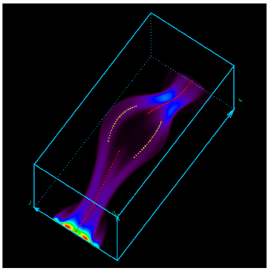
Figure 1: A volume rendering of $B^{2}$ for the last timestep of run SL0. The red dotted line denotes the central axis of the portion of the $\Omega$-loop which has not fragmented. The yellow dotted lines denote the paths of each distinct fragment in the region of the loop that is considered to be fragmented. The entire rectangular computational domain is shown.

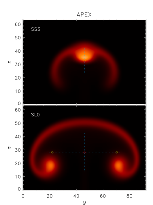
Figure 2: The apex cross-sections of the $\Omega$-loops shown in Figure 1 (bottom panel) and Figure 3 (top panel). The symbols denote the positions of the tube axes, and the lengths of the blue dotted lines represent the second moments of the field distribution centered on the tube centroid (see equation [3]). These lines serve as a visual measure of the degree of fragmentation. The $x$ and $y$ scale is given in terms of computational zones.

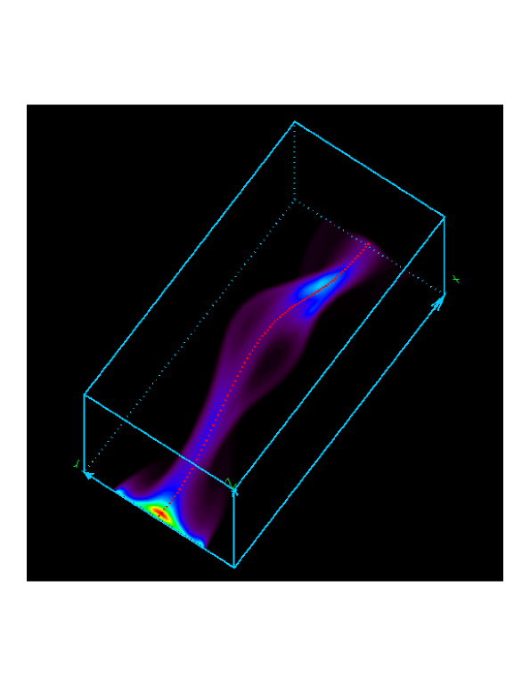
Figure 3: A volume rendering of $B^{2}$ for the last timestep of run SS3. The red dotted line denotes the central axis of the non-fragmented flux tube.

From an examination of numerous simulations, we empirically find that a magnetic flux tube can be considered to have split apart when its deformation, $f$, exceeds 1.5. We therefore use $f$ as our measure of the degree of fragmentation of the tube, consistent with the results of Schüssler (1979) and Longcope, Fisher, & Arendt (1996). If $f>1.5$, then the path of each individual flux tube fragment is calculated using equations (3) and (20) over subdivided portions of the surface $S$. Since there is a fairly high degree of symmetry in our runs, the surface can be divided into two parts that lie on either side of a line defined by the Frenet normal. Thus, the regions of integration are easily determined. Figure 1 is a volume rendering of the magnetic field strength for the final timestep of run SL0, and shows the geometry of a tube which has fragmented as it rises toward the surface. The field strength distribution is visualized by casting parallel rays through the semi-transparent volume, and calculating the two-dimensional projection onto the viewing plane (IDL’s “voxel_proj” routine). The red dotted line denotes the central axis of the tube through the volume. Where the tube has fragmented, yellow dotted lines trace the paths of each fragment. Note that the axis of each tube fragment does not coincide exactly with their centers of vorticity (where the field strength is locally concentrated); this offset depends on the amount of flux that resides in a thin “sheath” that extends from the forefront of the rising tube to the outer edge of each vortex pair. These features can be seen in a cross-section at the apex of this $\Omega$-loop in the bottom frame of Figure 2. In this case, the magnetic sheath is revealed as a relatively weak concentration of flux in the shape of a thin, semi-circular arch that lies above the primary concentrations of flux located in the trailing eddies. The yellow symbols denote the location of the central axis of each fragment, and the lengths of the blue dotted lines represent the second moments of the field distribution (given by equation [3]) at the centroid of the tube (note that at the apex of the loop, $\hat{n}$ and $\hat{b}$ approximately correspond to the Cartesian directions $\hat{z}$ and $\hat{y}$ respectively). The top panel of Figure 2 shows the apex cross-section of the flux tube shown in Figure 3 (the final timestep of run SS3). This is an example of a tube which, by our definition, has not yet fragmented as it approaches the photospheric boundary.

3.1 How Fragmentation Depends on Tube Curvature and Twist

To investigate how the degree of fragmentation at the apex of a rising, magnetic flux tube depends on its curvature at that point, we consider five separate runs: SS1, SL1, LS1, LL1, and L1. In each case, the initial twist parameter $q$ is taken to be $1/8$; that is, the simulations begin with identical, weakly-twisted horizontal flux tubes positioned at the same depth near the bottom of the computational domain. Effectively, the difference between each run is the length in the axial direction of the rising portion of the flux tubes. The changes in this length scale lead to substantive differences in the apex curvature of the $\Omega$-loop as it rises through the stratified atmosphere. Run L1 (the two-dimensional limiting case) represents an infinitely long horizontal tube whose apex curvature remains zero throughout its rise. Conversely, run SS1 represents the shortest length scale we have considered, and thus refers to the run with the highest apex curvature as the tube approaches the photosphere.

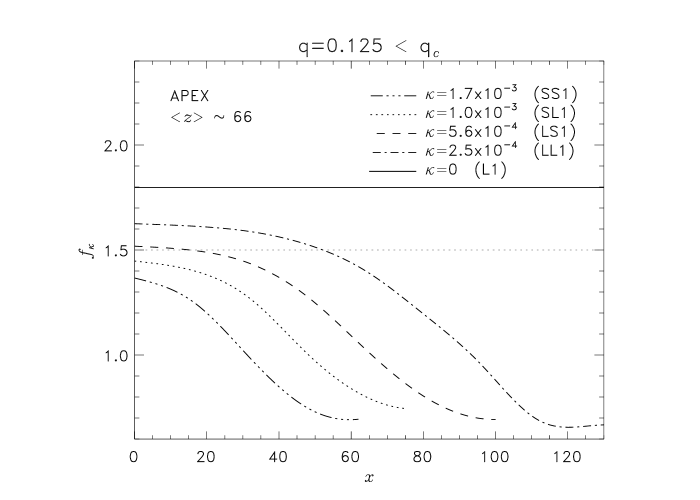
Figure 4: Fragmentation as a function of curvature for $q=1/8$. The $x$ scale is given by the number of computational zones from each tube’s apex, and $<\!\!z\!\!>$ is the average height of the central axis of the tubes (given in terms of the number of computational zones from the lower boundary). For clarity, the $f$ values near the horizontal boundaries of each run (past the end of the $\Omega$-loop) are not shown.

Figure 4 shows the degree of fragmentation along the axis of each tube for these five values of apex curvature at the time when each tube has risen approximately half-way through the vertical extent of the domain. In order of decreasing curvature, the simulations shown are runs SS1, SL1, LS1, LL1, and L1. The line $f=1.5$ represents the (somewhat arbitrary) point at which we consider the tube to be fragmented. It is easy to see that as the level of apex curvature $\kappa$ increases, the less the tube fragments for a fixed value of $q$. Figure 4 also shows that although the initial value of twist was slight, three of the four simulations have yet to show clear signs of fragmentation at the apex of the loop. This suggests that in three dimensions, the amount of twist necessary to prevent fragmentation is substantially reduced from the two-dimensional value — a point that we will return to later in this section. Note that toward the footpoints of each loop, the value of $f_{\kappa}$ falls below $1$ (the $\kappa$ subscript is included to emphasize the dependence of the degree of fragmentation $f$ on the tube’s apex curvature $\kappa$). This reflects the net elongation of the tube cross-section in the $\hat{n}$ direction as the $\Omega$-loop expands.

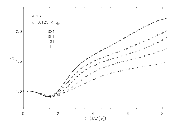
Figure 5: Apex fragmentation as a function of time and apex curvature for the set of runs where $q=1/8$.

Figure 5 shows the time dependence of $f_{\kappa}$ at the loop apex for the set of runs corresponding to those of Figure 4. A striking feature of this plot is the reduction by a factor of $\approx 1.5$ in the degree of fragmentation near the photospheric boundary between the run with zero apex curvature, and the run with the maximum amount of curvature. The difference in $f_{\kappa}$ is large enough that the magnetic flux emerges as two individual fragments when $\kappa=0$ (run L1), yet is closer to being a single, cohesive tube when $\kappa\gtrsim 1.7\times 10^{-3}$ (run SS1). Note that during the initial stages of the run, before the tube shows signs of fragmentation, $f_{\kappa}$ falls slightly below $1$. This is a result of the vertical elongation of the apex cross-section as the tube begins to rise, and flux is pulled into its wake.

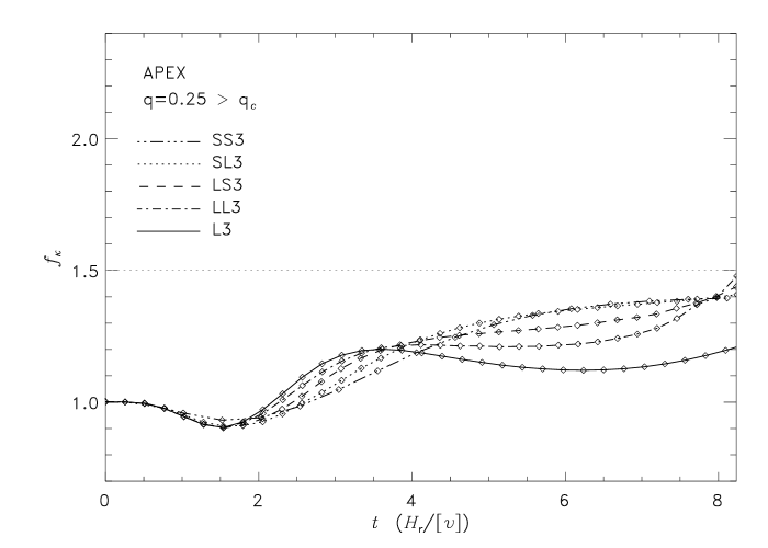
Figure 6: Apex fragmentation as a function of time and apex curvature for the set of runs where $q=1/4$.

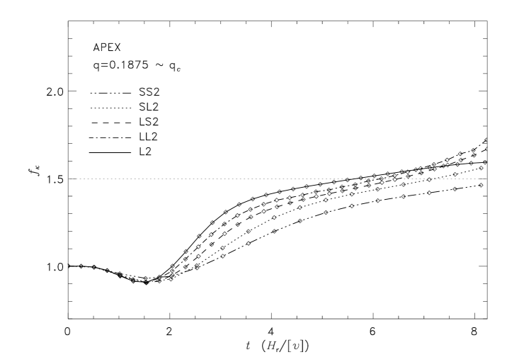
Figure 7: Apex fragmentation as a function of time and apex curvature for the set of runs where $q=3/16$.

We find that if the initial value of the twist parameter $q$ is greater than a “critical” value, $q_{c}$, then the flux tube no longer emerges in a fragmented state, ($f<1.5$) regardless of the radius of curvature of the loop (see Figure 6). In our simulations, $q_{c}$ is empirically determined to be only slightly less than $3/16$, the value chosen for the set of runs SS2, SL2, LS2, LL2, and L2 of Figure 7. For the two-dimensional limiting cases, the empirically determined critical value is consistent with the condition that the flux tube will split apart when the rise velocity of the tube exceeds the Alfvén speed of the azimuthal field at its edge (note that the initial entropy perturbation in our simulations will affect the rise speed of the tube). However, if the initial twist of the flux tube is less than $q_{c}$, we find that the curvature of the $\Omega$-loop plays an important role in determining the degree of fragmentation of the tube prior to its emergence through the photosphere — an effect not accounted for in previous two-dimensional studies of flux tube fragmentation (eg. Longcope, Fisher, & Arendt 1996, Emonet & Moreno-Insertis 1998, and Fan, Zweibel, & Lantz 1998). A comparison of Figure 7 with Figure 5 further suggests that as one chooses values of $q$ progressively less than $q_{c}$, the effect of loop curvature on the degree of apex fragmentation becomes more pronounced.

Run L1, the two-dimensional limiting case with a relatively small amount of initial field line twist, confirms the results of previous two-dimensional simulations (Longcope, Fisher, & Arendt, 1996; Emonet & Moreno-Insertis, 1998; Fan, Zweibel, & Lantz, 1998), which show that once fragmentation has occurred, the two counter-rotating fragments repel one another via forces that result from infinitely long vortex lines. In two dimensions, the horizontal separation of the fragments can be understood in terms of the hydrodynamic force acting on an object with a net circulation $\Gamma$ moving relative to a fluid with a velocity $v$: $\mathbf{F}=-\rho_{0}$$v$$\times$$\,\Gamma$  (see Fan, Zweibel, & Lantz 1998). It is the component of this “lift” force per unit volume acting along the line between the centers of vorticity of the tube fragments that acts to push the tubes apart. In three dimensions, the fragments are finite in extent, and thus these forces are important only over a finite length of the loop. Figure 8 shows the trajectory of the two fragments (for the weakly-twisted case) at the tube apex for five different values of curvature. As the level of apex curvature of the tube increases, and the effective axial length scale of each vortex pair decreases, we see that the total volume integrated non-vertical component of the hydrodynamic lift — and thus the fragment separation — is reduced.

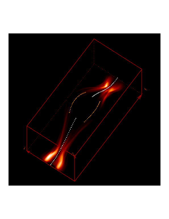
Figure 9: A volume rendering of the current helicity for the last timestep of run SL0. The dotted lines denote the paths of both the fragmented and un-fragmented portions of the loop. The entire rectangular computational domain is shown.

Field line twisting due to non-uniform rotation of the fragments also acts to reduce the fragment separation. To illustrate the role of field line twist in the interaction of the vortex pairs, we consider a case where the azimuthal component of the magnetic field along the tube is initially zero. Figure 9 is a volume rendering of the magnitude of the current helicity density ($|H_{\mathrm{c}}|=|\mathbf{J}\cdot\mathbf{B}|$, where $\mathbf{J}=\nabla\times\mathbf{B}$) for the final timestep of run SL0 (where $q\equiv 0$). Since the current helicity gives a measure of the twist of the magnetic field, Figure 9 shows that after the tube rises, spins differentially (see Figure 10), and splits apart, the magnetic field along each tube fragment becomes increasingly twisted. The magnetic forces imparted from the increased twist slow the rotational motion of the vortex pairs, and thus the tendency for the tubes to separate is further reduced. Figure 11 shows that as the apex curvature of the $\Omega$-loop increases, the net circulation near the apex of each fragment decreases. This lessens the repulsive force between fragments, and allows $\Omega$-loops with a high degree of apex curvature to behave more cohesively. This suppression of circulation in the tube fragments was predicted by Emonet & Moreno-Insertis (1998) and Moreno-Insertis (1997), who suggested that if the footpoint separation of an $\Omega$-loop was small enough, the rotation of the vortex pairs would be suppressed. Since it is reasonable to assume a correlation between footpoint separation and apex curvature, we feel that the results of our simulations are generally consistent with this prediction.

3.2 Field Morphology Prior to Emergence

There are a number of reasons why one must be cautious when comparing our results with flux emergence observations. First, the anelastic approximation becomes marginal as the magnetic flux tube approaches the photosphere, where densities decrease to the point that local sound speeds are comparable to Alfvén speeds in the plasma. Additionally, in this first generation of models we do not include the effects of spherical geometry or the Coriolis force. Thus, predicted asymmetries in the geometry and field strength asymmetry of emerging active regions (see Moreno-Insertis, Schüssler, & Caligari 1994 and Fan, Fisher & DeLuca 1993) will not be reproduced. Further, we choose to use a simple, polytropic reference state rather than a more realistic convective background. As a result, the effects of convective turbulence on the tube are neglected during its rise to the surface, likely over-simplifying the structure of the field. Nevertheless, we can make some general predictions regarding the morphology of emerging magnetic flux in active regions if the field exists in the form of a fragmented flux tube.

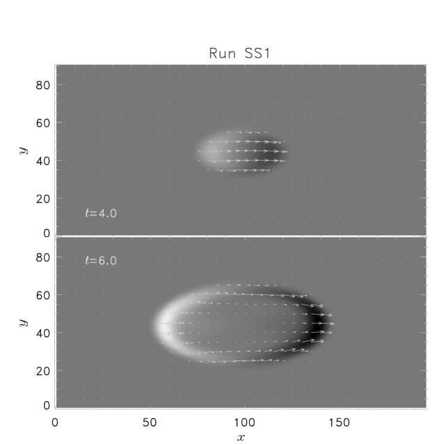
Figure 12: Vector magnetogram images for run SS1. The times given are in naturalized units ($t=H_{r}/[v]$, see text), and the $x$ and $y$ scale are given in terms of the computational grid. The grey-scale background represents the vertical component of the magnetic field (positive values are indicated by the light regions), and the arrows represent the transverse components.

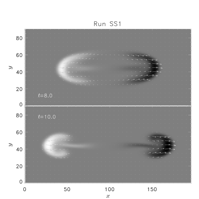
Figure 13: Same as Figure 12, for later timesteps.

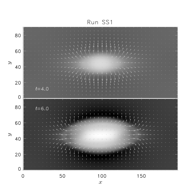
Figure 14: The velocity field for the same horizontal slice and times shown in Figure 12. The grey-scale background represents the vertical component of the velocity (light regions indicate positive values), and the arrows represent the transverse components of the velocity field.

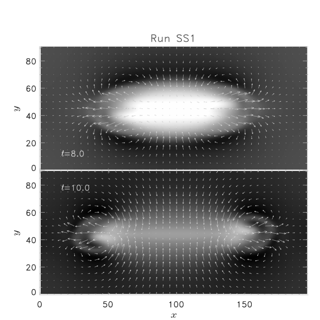
Figure 15: Same as Figure 14 for the times corresponding to Figure 13.

Figures 12 and 13 make up a time-series of simulated vector magnetograms for the rising, fragmented flux tube of run SS1. These images were generated by taking a horizontal slice as close to the top of the computational domain as possible without having the topological evolution affected by interaction with the upper boundary. The grey-scale background represents the vertical component of the magnetic field; light regions correspond to outwardly directed magnetic field (toward the observer), and dark regions correspond to inwardly directed field (away from the observer). The arrows define the direction and relative strength of the transverse components of the field. Figures 14 and 15 show the corresponding velocity field at the same time intervals and locations. The first frame of Figure 12 shows the tip of the magnetic sheath as it begins to cut through the horizontal plane. At this point, there is little to no separation between regions of opposite polarity, and the corresponding flow field surrounding the magnetic region is relatively weak. This stage is short-lived, since the magnetic sheath is very thin.

As the tube continues to rise, the horizontal cut passes through regions of magnetic field concentrated in the sheath on either side of the tube apex (which by now has emerged through the photosphere), as well as the field concentrated in the relatively horizontal trailing vortices of each fragment. As a result, an oval-like structure develops, as shown in frame 2 of Figure 12. The velocity field has a strong vertical component near the interfaces between the vortex tubes and the surrounding non-magnetized plasma, while exhibiting strong horizontal components at each end. The horizontal components reflect the flow of material along the sheath away from the apex (see frame 2 of Figure 14). In frame 1 of Figure 13, the apex of each individual fragment has passed through the cutting plane, and we see only the portions of the tube fragments and sheath located just above the $\kappa$ inflection point of the $\Omega$-loop. The two regions of opposite polarity now appear crescent-shaped as they continue to separate. After the fragmented portion of the loop has emerged through the photosphere, only the more concentrated, non-fragmented portions remain. Thus, in the final frame of Figure 13, the regions of strong magnetic field appear to have coalesced — a feature of emerging active regions that is commonly observed.

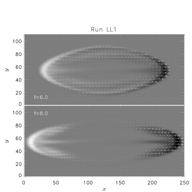
Figure 16: Vector magnetogram images for run LL1. The times given are in naturalized units ($t=H_{r}/[v]$, see text), and the $x$ and $y$ scale are given in terms of the computational grid. The grey-scale background represents the vertical component of the magnetic field (positive values are indicated by the light regions), and the arrows represent the transverse components.

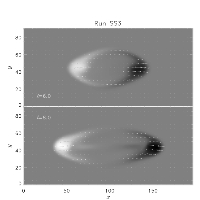
Figure 17: Same as Figure 16 for run SS3.

Figures 16 and 17 show a similar time-series of vector magnetograms for runs LL1 and SS3 respectively. A comparison between these figures and Figures 12 and 13 reveals the effect of initial twist and tube curvature on the overall characteristics of the emerging flux. A comparison of the surface separation of the individual fragments (the semi-minor axes of the ellipse-like structures shown in frame 2 of Figure 12 and frame 1 of Figure 16) can be used to determine the relative curvature between the two cases. In general, the lower the apex curvature of the fragmented $\Omega$-loop, the higher the “eccentricity” of the ellipse-like structure. Similarly, if the crescent-shape of the opposite polarity magnetic structures is less distinct or absent in the simulations (compare frame 1 of Figure 13 with frame 2 of Figure 17), this indicates that the initial level of twist of the magnetic flux tube was relatively high. Finally, asymmetries introduced by the higher level of twist present in the runs where $q=1/4$ can result in the emergence of bipolar regions that are tilted slightly with respect to the $\hat{x}$ direction. Note that a very slight tilt of approximately $4$ degrees from the horizontal has developed between the center of the bipolar regions shown in frame 1 of Figure 17.

Our description of a fragmented flux tube is in qualitative agreement with recent images of certain emerging active regions observed by Cauzzi, Canfield, & Fisher (1996), Strous & Zwaan (1999), and Mickey & Labonte (1999). Vector magnetograms and white-light images of flux emergence taken with high temporal resolution by the Imaging Vector Magnetograph at the University of Hawaii’s Mees Observatory (IVM) in relatively uncluttered portions of the solar disk (Mickey & Labonte, 1999) show evolving magnetic structures that are similar to the evolving structures described above. In particular, it is possible to infer the presence of oval-shaped magnetic features which evolve into crescent-shaped regions of opposite polarity that rapidly separate. In principle, direct measurements of the rate of separation and coalescence of the opposite polarity regions of the field may be used to obtain information about the structure and evolution of the sub-surface magnetic field. However, to perform this kind of detailed comparison with observation will require a more sophisticated set of models.

4 Summary and Conclusions

We have performed detailed numerical simulations of the rise of twisted magnetic flux tubes embedded in a non-magnetic, stratified plasma using a code which solves the three-dimensional MHD equations in the anelastic approximation. The evolving magnetic field is described in terms of its volumetric flux distribution as a magnetic flux tube which may fragment into separate, distinct tubes during its rise toward the photospheric boundary. We find that the degree of fragmentation of the evolving magnetic flux tube depends not only on the initial ratio of the azimuthal to axial components of the field along the tube (as was the case in two dimensions), but also on the three-dimensional geometry of the tube as it rises through the convection zone. The principal results of our analysis are the following:

1. If the ratio of azimuthal to axial components of the field along a magnetic flux tube exceeds a critical limit, then it will retain its cohesion and not fragment as it rises through the plasma. The critical limit occurs when the rise speed is approximately equal to the maximum Alfvén speed of the azimuthal component of the field. This reinforces the conclusions of Emonet & Moreno-Insertis (1998), Moreno-Insertis & Emonet (1996), Longcope, Fisher, & Arendt (1996), and Fan, Zweibel, & Lantz (1998).

2. If the initial amount of field line twist is less than the critical value, and if the magnetic flux tube rises toward the photosphere as an $\Omega$-loop, then the degree of apex fragmentation depends on the curvature of the loop — the greater the apex curvature, the lesser the degree of fragmentation for a fixed amount of initial twist.

3. In two dimensions, counter-rotating vortices are effectively infinite in extent and generate long-range flows which eventually prevent the continued vertical rise of tube fragments. This artificial geometric constraint is relaxed in three dimensions, and although the fragments continue to experience forces due to the interaction of the vortex pairs, those forces are only important along a short section of the tube. Thus, the fragments are able to rise to the surface. The forces due to vortex interaction depend upon the geometry of the $\Omega$-loop — the greater the apex curvature, the lesser their magnitude. Thus, highly curved loops exhibit less fragmentation during their rise.

4. Differential circulation between the apex and footpoint of an $\Omega$-loop leads to the introduction of new magnetic twist of opposite sign in each leg of a loop fragment. This twist reduces the circulation about the apex of each fragment, and further reduces the forces acting to separate the fragments of the flux tube. This result is consistent with the predictions of Emonet & Moreno-Insertis (1998) and Moreno-Insertis (1997).

5. Though these models do not admit to a direct, detailed comparison with observations, it is possible to infer certain general observational characteristics of emerging magnetic flux if the field configuration is that of a fragmented $\Omega$-loop rising through the solar surface. If the magnetic field erupts through a relatively quiet portion of the Sun, then we expect that one should observe concentrations of vertical flux which resemble expanding oval shapes. This type of feature should quickly evolve into longer-lived crescent-shaped regions of opposite polarity that steadily move away from one another. These extended regions should then coalesce once the fragmented portions of the $\Omega$-loop have emerged through the solar surface.

Figure 8: Fragment trajectories at the apex of the rising $\Omega$-loop for the set of simulations where $q=1/8$. Note that at the loop apex, the normal $n$ and binormal $b$ directions correspond approximately to the Cartesian directions $z$ and $y$ respectively. $\ell_{\rho}$ represents the trajectory expected from pure expansion and no vortex interaction. The axis scale is in terms of computational zones — an entire vertical slice of the domain is shown.

Figure 10: The magnitude of the net circulation of an individual tube fragment (normalized to its value at the tube’s apex, $\Gamma_{0}$) for the last timestep of run SL0.

Figure 11: The magnitude of the net circulation of a tube fragment (normalized to the value of run L1 at $t=7$, $\Gamma_{0}$) at the apex of the $\Omega$-loops as a function of apex curvature for the runs with a relatively small amount of initial field line twist.

Table 1: Initial Flux Tube Parameters

Label	Resolution	$L$	$\mathcal{L}$	$q$	$Q\!=\!\frac{Lq}{2\pi a}$	$\kappa$
SS1	256$\times$128$\times$128	4.362	0.0852	0.1250	0.8678	1.66248
SS2	256$\times$128$\times$128	4.362	0.0852	0.1875	1.3017	1.62260
SS3	256$\times$128$\times$128	4.362	0.0852	0.2500	1.7356	1.62906
SL0	256$\times$128$\times$128	4.362	0.1704	0.0000	0.0000	1.05930
SL1	256$\times$128$\times$128	4.362	0.1704	0.1250	0.8678	1.04928
SL2	256$\times$128$\times$128	4.362	0.1704	0.1875	1.3017	0.99512
SL3	256$\times$128$\times$128	4.362	0.1704	0.2500	1.7356	1.02579
LS1	512$\times$128$\times$128	8.724	0.1704	0.1250	1.7356	0.53913
LS2	512$\times$128$\times$128	8.724	0.1704	0.1875	2.6034	0.51325
LS3	512$\times$128$\times$128	8.724	0.1704	0.2500	3.4712	0.46269
LL1	512$\times$128$\times$128	8.724	0.3408	0.1250	1.7356	0.23734
LL2	512$\times$128$\times$128	8.724	0.3408	0.1875	2.6034	0.20638
LL3	512$\times$128$\times$128	8.724	0.3408	0.2500	3.4712	0.16699
L1	2$\times$128$\times$128	$\infty$	$\infty$	0.1250	$\infty$	0.00000
L2	2$\times$128$\times$128	$\infty$	$\infty$	0.1875	$\infty$	0.00000
L3	2$\times$128$\times$128	$\infty$	$\infty$	0.2500	$\infty$	0.00000

References

- Bercik, Stein, & Nordlund (1999) Bercik, D., Stein, R. F., & Nordlund, A., 1999, American Astronomical Society Meeting, 194, 5501.
- Caligari, Moreno-Insertis, & Schüssler (1995) Caligari, P., Moreno-Insertis, F., & Schüssler, M., 1995, ApJ, 441, 886.
- Cauzzi, Canfield, & Fisher (1996) Cauzzi, G., Canfield, R. C., & Fisher, G. H., 1996, ApJ, 456, 850.
- Cauzzi, Moreno-Insertis, & van Driel-Gesztelyi (1996) Cauzzi, G., Moreno-Insertis, F., & van Driel-Gesztelyi, L., 1996, Astron. Soc. Pac. Conf. Series, 109, 121.
- Corbard et al. (1999) Corbard, T., Blanc-Feraud, L., Berthomieu, G., Provost, J., 1999, A&A, 344, 96.
- D’Silva & Choudhuri (1993) D’Silva, S., & Choudhuri, A. R., 1993, A&A 272, 621.
- D’Silva & Howard (1993) D’Silva, S., & Howard, R. F., 1993, Sol. Phys., 148, 1.
- DeLuca & Gilman (1991) DeLuca, E. E., & Gilman, P. A., 1991, in Solar Interior and Atmosphere, Tucson AZ, University of Arizona Press, 275.
- Dikpati & Charbonneau (1999) Dikpati, M., & Charbonneau, P., 1999, ApJ, 518, 508.
- Dorch & Nordlund (1998) Dorch, S. B. F., & Nordlund, A., 1998, A&A, 338, 329.
- Durney (1997) Durney, B. R., 1997, ApJ, 486, 1065.
- Emonet & Moreno-Insertis (1998) Emonet, T., & Moreno-Insertis, F., 1998, ApJ, 492, 804.
- Fan (1999) Fan, Y., 1999, ApJ, submitted
- Fan & Fisher (1996) Fan, Y., Fisher, G. H., 1996, Sol. Phys., 166, 17.
- Fan, Fisher & DeLuca (1993) Fan, Y., Fisher, G. H., & DeLuca, E. E., 1993, ApJ, 405, 852.
- Fan et al. (1999) Fan, Y., Zweibel, E. G., Linton, M. G., & Fisher, G. H., 1999, ApJ, 521, 460.
- Fan, Zweibel, & Lantz (1998) Fan, Y., Zweibel, E. G., & Lantz, S. R., 1998, ApJ, 493, 480.
- Ferriz-Mas & Schüssler (1993) Ferriz-Mas, A., & Schüssler, M., 1993, in Geophys. Astrophys. Fluid Dyn., 72, 209.
- Ferriz-Mas & Schüssler (1995) Ferriz-Mas, A., & Schüssler, M., 1995, in Geophys. Astrophys. Fluid Dyn., 81, 233.
- Fisher, Fan & Howard (1995) Fisher, G. H., Fan, Y., & Howard, R. F., 1995, ApJ, 438, 463.
- Frigo & Johnson (1997) Frigo, M., & Johnson, S. G., 1997, “The Fastest Fourier Transform in the West”, in report MIT-LCS-TR-728, Massachusetts Institute of Technology.
- Gilman, Morrow, & DeLuca (1989) Gilman, P. A., Morrow, C. A., & DeLuca, E. E., 1989, ApJ, 338, 528.
- Glatzmeier (1984) Glatzmeier, G. A., 1984, J. Comput. Phys., 55, 461.
- Gough (1969) Gough, D. O., 1969, J. Atmos. Sci., 26, 448.
- Kosovichev (1996) Kosovichev, A. G., 1996, ApJ, 469, L61.
- Lantz & Fan (1999) Lantz, S. R., & Fan, Y., 1999, ApJS, 121, 247.
- Linton, Longcope, & Fisher (1996) Linton, M. G., Longcope, D. W., & Fisher, G. H., 1996, ApJ, 469, 954.
- Longcope & Fisher (1996) Longcope, D. W., & Fisher, G. H., 1996, ApJ, 458, 380.
- Longcope, Fisher, & Arendt (1996) Longcope, D. W., Fisher, G. H., & Arendt, S., 1996, ApJ, 464, 999.