The CNOC2 Field Galaxy Redshift Survey I: The Survey and the Catalog for the Patch CNOC 0223+00

Abstract

The Canadian Network for Observational Cosmology (CNOC2) Field Galaxy Redshift Survey is a spectroscopic/photometric survey of faint galaxies over 1.5 square degrees of sky with a nominal spectroscopic limit of $R_{c}\sim 21.5$ mag. The primary goals of the survey are to investigate the evolution of galaxy clustering and galaxy populations over the redshift range of $\sim 0.1$ to $\sim 0.6$. The survey area contains four widely separated patches on the sky with a total sample of over $6000$ redshifts, representing a sampling rate of about 45%. In addition, 5-color photometry (in $I_{c}$, $R_{c}$, $V$, $B$, and $U$) for a complete sample of approximately 40,000 galaxies to $R_{c}\sim 23.0$ mag is also available. We describe the survey and observational strategies, multi-object spectroscopy mask design procedure, and data reduction techniques for creating the spectroscopic-photometric catalogs. We also discuss the derivations of various statistical weights, including corrections for the effects of limited spectral bandwidth, for the redshift sample which allow it to be used as a complete sample. As the initial release of the survey data, we present the full data set and some statistics for the Patch CNOC 0223+00.

1 Introduction

Fundamental to our understanding of the Universe is the formation and evolution of structures, from galaxies to clusters of galaxies to large-scale structures such as sheets, filaments, and voids. Theoretical advances, often in the form of increasingly larger and more sophisticated N-body simulations, have laid much of the groundwork in interpreting the development and evolution of dark matter clustering (e.g., Davis et al. 1985; Colin, Carlberg, & Couchman 1997; and Jenkins et al. 1998). The modeling of the connection between the clustering of galaxies (which are the most easily observed component) and dark matter (which provides the gravitational field), however, is complex and much less well understood. In essence, deriving such a connection requires a full understanding of galaxy formation and evolution.

On the observational side, progressively larger redshift surveys of galaxies have provided relatively robust measurements of the present-epoch galaxy correlation function or power spectrum (e.g., the CfA survey [Davis & Peebles 1983, Vogeley et al. 1992]; and the LCRS [Lin et al. 1996]). Although there has been a number of investigations attempting to measure the evolution of galaxy clustering out to $z\sim$ 0.5 to 1.0, they were all based on small surveys which were not specifically designed for this purpose (e.g., LeFèvre et al. 1996, Shepherd et al. 1997, Carlberg et al. 1997). These surveys cover very small areas with sample sizes of 100’s of objects. Furthermore, the substantial galaxy population evolution over this redshift range must be taken into account to ensure that similar samples of galaxies at different redshifts are being used to measure the clustering evolution.

The second Canadian Network for Observational Cosmology (CNOC2) Redshift Survey is the first large redshift survey of faint field galaxies carried out with the explicit goal of investigating the evolution of clustering of galaxies. Such an investigation requires a sample with a large number of galaxies spanning a significant redshift range and covering a sufficiently large area on the sky. The redshift range over which the evolution is to be measured is 0.1 to 0.6, chosen to maximize the efficiency of a 4m class telescope. The survey is also designed specifically to provide a large database of both spectroscopy and multicolor photometry data for the study of the evolution of galaxy populations over the same epochs. This is particularly important as such information will allow us to attempt to disentangle any inter-dependence between the correlation function and galaxy types and evolution.

The current knowledge of field galaxy evolution at $z\sim 0.5$ is based mostly on the measurement of the luminosity function (LF) (e.g., Lilly et al. 1995; Ellis et al. 1996; Lin et al. 1997), with the primary conclusion being that the most rapid evolution is seen in blue, star-forming galaxies. A much larger redshift sample of several thousand galaxies with multi-color photometry will vastly improve on the current results. The multicolor data can provide sufficient information to allow a classification of the spectral energy distributions of the sample galaxies. This, along with a large sample size, will make possible a much more detailed analysis of the evolution of the LF as a function of galaxy population, perhaps enabling a definitive discrimination between luminosity and density evolution.

In this paper, we describe the general strategy and design of the CNOC2 survey, the data reduction methods, and the creation of weight functions. Also presented is the first data catalog from the survey. In Section 2 we present the survey strategy, the field selections and the observations. Sections 3 and 4 describe the data reduction methods for the photometric and spectroscopic data, respectively. The issues of completeness and weights are discussed in Section 5. Finally, Section 6 presents the catalog for the patch CNOC 0223+00. First results on galaxy population evolution and clustering evolution are presented in papers by Lin et al. (1999) and Carlberg et al. (2000), respectively. Reports on close-pair merger evolution and the serendipitous active galactic nuclei sample from the survey are given in papers by Patton et al. (2000) and Hall et al. (2000). Additional papers on more detailed studies of galaxy evolution, the dependence of clustering evolution on galaxy types, and other related subjects are in preparation.

2 The Survey

The CNOC2 Field Galaxy Redshift Survey was conducted using the MOS arm of the MOS/SIS spectrograph (LeFèvre et al. 1994) at the 3.6m Canada-France-Hawaii Telescope (CFHT). The primary goal of the survey is to obtain a large, well-defined sample of galaxies with high quality spectroscopic and photometric data for the purpose of studying the evolution of galaxy clustering in the redshift range of $\sim 0.1$ to 0.6. To first order, such a goal requires a survey at these intermediate redshifts which is comparable to the local universe CfA redshift survey (Huchra et al. 1983, Geller & Huchra 1989) in the number of galaxies ($\sim 10^{4}$), the volume covered ($\sim 10^{6}h^{-3}$ Mpc³), and velocity accuracy ($\sim 50$ km s^-1).

The redshift range for the survey is chosen to maximize the spectroscopic efficiency of a 4m class telescope and the MOS spectrograph. Based on the experience from the CNOC1 Cluster Redshift Survey (Yee, Ellingson, & Carlberg 1996; hereafter YEC), a relatively high success rate of $\sim 85$% can be obtained with a reasonable exposure time of the order of an hour for galaxies at $R_{c}\sim 21.5$. Such a sample would have an average galaxy density on the sky of $\sim$ 145 galaxies per MOS field (of about 70 square arcminutes), and a peak of $z\sim 0.35$ in the redshift distribution, well-matched to the number of slits available in the MOS field and the redshift range.

The robust measurement of the spectral energy distributions (SED) of the sample galaxies in the form of multi-color photometry is also an integral part of the survey. Furthermore, the availability of multicolor photometry will allow us to produce a photometric-redshift training set of unprecedented size, and also provide important consistency checks on the spectroscopic redshift measurements. Hence, a significant amount of telescope time is also devoted to imaging in the survey. In the following subsections, we describe the main features of the survey in detail.

2.1 Field Selections

There are several considerations in choosing the survey areas on the sky. To avoid being dominated by a small number of large structures, the survey covers four widely separated regions, called patches, on the sky. There are a number of advantages in splitting the sample area into 4 regions. First, this allows one to obtain a reasonable sampling of the clustering; this is particularly important because each of the patches still covers a relatively small area on the sky. Second, having 4 patches provides a rough estimate of the cosmic variance in the determination of the clustering and statistical properties of galaxies such as the luminosity function, luminosity density, and star formation rate. In the case of clustering, the different patches will also provide an indication as to whether there are significant clustering signals at scales larger than the area covered by a single patch. Finally, having 4 patches allows us to distribute them in Right Ascension to maximize observing efficiency.

For a sample of the order of $\sim 10^{4}$ galaxies over a volume of $\sim 10^{6}h^{-3}$ Mpc³, we need to cover the order of at least 1.5 square degrees. Hence, each patch should have an area of about 0.4 square degrees. One pointing of the MOS field, after considerations of spectral coverage on the CCD, provides a spectroscopically defined area of about $9^{\prime}\times 7^{\prime}$, with about 15^′′ overlapping area with the adjacent fields. Thus, each patch is equivalent to about 20 MOS fields.

To obtain a sufficiently large length scale for determining the correlation function reliably, we also need each patch to extend about 10 to 20 $h^{-1}$Mpc over our redshift range. These considerations motivated us to design the geometric shape of each patch to have a central block of about 0.5^o$\times$0.5^o with two orthogonal “legs” extending outward, as illustrated in Figure 1. Each patch, as designed, spans $\sim 80^{\prime}$ and $\sim 63^{\prime}$ in the North-South and East-West direction, respectively. We have named the fields in each patch as indicated in Figure 1 (along with the sequential field numbers), with the a fields representing the North arm, the b fields representing the East portion of the central block, and the c fields representing the West edge and arm. The somewhat peculiar naming of the b fields is due to the initial design of the patch having an inverted $Y$ shape, and the name b was used to designate the East arm. The patch design was altered after the first run in order to include a central block, so that the b arm has effectively “curled” into the middle to form the central block.

Figure 1: Geometric shape of a patch and the designations of fields. North-East is upper left. The field size is based on that for the STIS2 CCD; fields taken with the ORBIT1 and LORAL3 CCDs are slightly smaller in the Declination direction. Although the c8 field was included in the original design, none of the patches actually contains one.

The properties of the patches are listed in Table 1. The four patches are selected based on several criteria. They are chosen to avoid bright stars ($m\lower 0.43057pt\hbox{\hbox to0.0pt{\raise 2.58334pt\hbox{\hskip 1.29167pt{{$\scriptscriptstyle<$}}}\hss} \kern-1.72218pt{{$\scriptscriptstyle\sim$}}}12$), low-redshift clusters (e.g., Abell clusters) and other known low-redshift bright galaxies, and known quasars and AGN. The patches have Galactic latitudes between 45^o and 60^o. The lower bound guards against excessive Galactic extinction ($<0.15$ mag in $A_{B}$). The extinction in the direction of each patch is obtained from the dust maps of Schlegel, Finkbeiner, & Davis (1998) and listed in Table 1 (see Lin et al. 1999 for details). The upper bound is chosen to ensure that there are a sufficient number of stars in each MOS field to provide proper star-galaxy classification. A significant number of stars are needed because of the variable point-spread function (PSF) over the MOS field (see Section 3.2).

The positions of the patches are chosen so that they are 5 to 7 hours apart in Right Ascension. This allows two patches to be accessible on the sky at any time of the year, and ensures that observations can be made within reasonable hour angles at any part of a given night. A total of 74 fields out of the intended 80 were observed for the survey, meeting 92.5% of the initial design goals.

2.2 Observations

We use the observational techniques developed for the CNOC1 Cluster Redshift Survey (YEC), with some additional improvements to increase the efficiency and in the sample selection method. The survey was carried out at the CFHT 3.6m telescope using the MOS imaging spectrograph. The survey was completed over a total of 53 nights in 7 runs from February 1995 to May 1998, with approximately 32 usable nights. Three different CCDs were used over the lifetime of the survey. Some pertinent properties of the CCDs are listed in Table 2 and a journal of the observations is presented in Table 3.

Three CCDs were used due to various reasons. Initially, the ORBIT1 CCD, a high quantum efficiency (QE) and blue sensitive detector, was used for run no. 1. However, it died just before run no. 2, and the older LORAL3, which has lower QE and poor blue sensitivity, was pressed back into service for both runs no. 2 and 3. From runs no. 4 to 7, the new STIS2 CCD became available. This is a high QE and blue sensitive detector with very clean cosmetic characteristics, but with a larger pixel size. Although the STIS2 CCD is a 2048$\times$2048 detector, the total size is significantly larger than the available field of view of MOS, and hence only a portion of the CCD was used. We note that the majority of the data (78%) were obtained using the STIS2 CCD, as the first 3 runs were plagued by bad weather. The exposure times for both spectroscopic and direct images were adjusted to compensate for the different QEs of the CCDs.

The MOS spectrograph has a usable field of about 10^′ diameter with the corners being in poor focus. An area smaller than the total imaging area is defined as the spectroscopic field, which is the area used for the survey. This defined spectroscopic area is limited by the CCD detector’s extent in spectral coverage, in that slits placed on different parts of the chip must all produce a complete spectrum. The spectroscopic field size for each detector is listed in Table 2. The defined area of adjacent fields are nominally overlapped 10^′′ to 20^′′ to provide consistency checks on astrometry, photometry, and redshift determination. Note that the STIS2 CCD has a significantly larger defined area because of the larger physical CCD size allowing for additional areas for the spectra of objects at the edge of the imaging field.

As in the CNOC1 survey, we use a band-limiting filter to increase significantly the multiplexing efficiency of the survey. The shortened spectra allow for multi-tiering of spectra on the CCD image, increasing the number of slits per spectroscopic mask from the order of 30 to about 100. For the CNOC2 survey, we have designed a filter with band limits of $\sim$ 4300Å to 6300Å. These limits were chosen with various compromises in mind. The range must be short enough to allow for significant multi-tiering, but long enough to be able to sample the key galaxy spectral features over a redshift range commanded by an apparent magnitude limit which is optimal for a 4m class telescope. Furthermore, the filter limits were chosen to coincide with the onset of the grism/CCD inefficiency in the blue, and with the first prominent atmospheric OH emission complex in the red. The transmission curve of the band-limiting filter is shown in Figure 2. The half-power limits for the curve are 4387Å and 6285Å with a peak transmission of $\sim 0.8$.

Figure 2: Transmission curve for the band-limiting filter for spectroscopy measured by observing a standard star.

The band limits effectively define the redshift completeness boundaries of the survey. The most prominent spectral features in galaxies over these wavelengths are [OII]$\lambda 3727$ for late-type galaxies and the Ca II H K features at $\lambda\lambda$3933,3969Å for early-type galaxies. For the HK lines, the effective redshift range is about 0.12 to 0.55. Although the [OII] line disappears at the blue edge at $z\sim 0.16$, the effective low redshift boundary for emission-line galaxies is $z\sim 0$, since for most emission-line objects, detectable [OIII]$\lambda\lambda$4959,5007Å move into the red end of the spectrum at $z\sim 0.25$. Hence, the effective redshift range for the full sample is 0.12 to 0.55; whereas it is 0.0 to 0.68 for emission line galaxies.

The imaging observations are carried out using 5 filters: $I_{c}$, $R_{c}$, $V$, $B$, and $U$, with typical integration times for each CCD listed in Table 2. (For simplicity, the subscript denoting the Cousins $R$ and $I$ filters will be dropped for the remainder of the paper.) The $V$ images are actually obtained through a Gunn $g$ filter, but calibrated to the Johnson $V$ system (see Section 3.1). The $R$ and $B$ images are utilized for designing the masks used for the spectroscopic observations. Image quality ranges from 0.7^′′ FWHM to 1.2^′′ in the best focused part of the $R$ images, with a deterioration up to about 20% near the edges due to the focal reducer optics.

The imaging data are reduced at the telescope, and preliminary catalogs of each field are produced and used to design the masks for multi-object spectroscopy. The mask design procedure, using a computerized algorithm, is described in Section 2.3. The MOS/SIS system at CFHT has a computer controlled laser slit cutting machine (LAMA), which allows spectroscopic masks with as many as 100 slits to be fabricated in 20 to 40 minutes. The elapsed time between obtaining a set of direct images to having a mask for spectroscopic observation, including the procedures for preprocessing, catalog creation, mask design, and mask cutting, was pushed to as low as about 2 hours by the end of the survey.

The new B300 grism is used for spectroscopy. This grism has enhanced blue response compared to the O300 grism used for CNOC1. Along with the blue sensitive CCDs, this produces a significant improvement in the blue region of CNOC2 spectra. The grism is blazed at 4584Å, and has a dispersion of 233.6Å/mm, giving 3.55Å/pixel for the ORBIT1 and LORAL3 CCDs, and 4.96Å/pixel for the STIS2 CCD. A slit width of 1.3^′′ is used for the spectroscopic observation, giving a spectral resolution of $\sim$14.8Å.

The observing procedure is similar to that for the CNOC1 survey (YEC). Two masks are observed for each field, with nominal integration times differing by a factor of $\sim 2$ between the A and B masks. Table 2 lists the spectroscopic integration times used for each CCD. Because the need to have continuously available a set of masks for spectroscopic observations prepared in advance, to maximize the observation efficiency, a computered-aided schedule of the imaging and spectroscopic observation sequence for each night is prepared ahead of time, and adjusted as weather, equipment failure, and varying acquisition and set-up time required. With the STIS2 CCD which has higher QE and faster readout time, on average for each field, including overhead for acquisition, focusing, mask alignment, and arc lamp calibration, $\sim$155 minutes were need for the spectroscopic observation of two masks, allowing as many as 800 spectra to be obtained in a single 10-hour clear night. For the direct imaging, $\sim$60 minutes were required for each field.

2.3 Galaxy Sample and Mask Design

A computerized mask design algorithm is used for generating the positional information of the slits for the fabrication of masks. Besides allowing one to optimize the placement of as many as 100 slits per mask, an objective design algorithm based on properly calibrated photometric catalogs also serves the very important task of producing a well-understood and well-defined spectroscopic galaxy redshift sample. The algorithm for optimal slit placement is identical to that used for CNOC1 (YEC); however, the selection process for the galaxy sample is different, and is specifically designed to generate a fair field-galaxy sample based on both the $R$ and $B$ photometry. The mask design uses only objects classified as galaxies with occasional stars included, either serendipitously (e.g., falling into a slit designed for a galaxy), or due to misclassification (see Sections 3.1 and 3.2).

Two masks, A and B, are designed for each field. For 4 of the 74 fields, a third mask C is also observed when either mask A or B are deemed insufficient due to poor observing conditions. The total number of masks observed in each patch is listed in Table 2. The nominal spectroscopic limit is $R=21.5$ and $B=22.5$. The defined sample for the spectroscopic survey is the union set of the two limits. Objects fainter than both of these limits belong to the secondary sample, for which slits are placed only if sufficient room for the spectrum is available on the detector.

The two-mask strategy for multi-object spectroscopy offers three important advantages. First, by choosing objects with different average brightnesses for the two masks, the integration time for each mask can be geared to the brightness of the objects, resulting in a significant saving of exposure time. Second, the second mask allows for the compensation of under-representation of close pairs in selecting objects for spectroscopic observation. This under-representation arises from the fact that once a slit is placed, a certain area on the CCD is blocked by the resulting spectrum of the object. This blockage as a function of the distance from a chosen object is illustrated by the thin solid line on Figure 3 which is derived based on the area blocked by the spectrum as a function of radius from the center of the slit. The discontinuity arises from the spectral coverage not being symmetric with respect to the central wavelength. This function is equivalent to the pair fraction expected in a spectroscopic sample created by a single mask from a parent photometric sample distributed uniformly on the sky. The actual situation is worse in that galaxies are clustered on the sky. The use of the second mask allows objects being blocked by the spectra in the first mask to be observed. This is a particularly important feature, in that without such compensation, a fair sampling of object separations is not possible, rendering severe selection effects in the correlation function. Finally, a second mask allows for the redundant observations of a significant number of objects, which is important for both quality control and obtaining empirical estimates of redshift measurement uncertainties.

Figure 3: Pair distributions for galaxies with $R_{c}\leq 21.5$ mag as a function of separation for the whole survey. The pairs are counted in individual fields and summed. This provides an indication of the effect of the mask design algorithm. Each distribution is plotted in pair fraction relative to the total photometric pair distribution, normalized to 1.0 at the radius of 220 arcsecond. The dot-dashed line represents the distribution of the A mask sample, while the dashed line shows the distribution of the total slit sample (i.e., both A and B masks) selected by the mask design algorithm. The light solid line is the theoretical distribution computed based on the fraction of area blocked by a single spectrum as a function of radius from the center of the slit. It represents the expected pair distribution arising from a uniformly distributed sample of galaxies selected using a single mask. The thick solid line represent the pair fraction distribution of the redshift sample. See the text for a detailed discussion of these distributions.

Mask A is designed with the emphasis on brighter galaxies, and has a total integration time of about 1/2 of that for Mask B. The design of mask A is based strictly on the apparent magnitude of the galaxies. A priority list of galaxies brighter than $R=20.25$ mag is made, with the objects closer to $R=20.25$ mag having the higher priorities. Slits which produce non-overlapping spectra are placed based on the order from this list.

This simple algorithm, however, produces the undesirable effect that objects near the upper and lower edges in the dispersion direction (i.e., the north and south edges) will preferentially have a higher probability of being placed. This arises because the spectra of these objects will extend beyond the defined field area on the CCD, effectively reducing the probability of their spectrum being blocked by those belonging to objects already chosen. To compensate for this edge effect, whenever a galaxy is chosen, the fraction of its spectrum falling outside the defined field is computed. The object is not accepted, and placed at the end of the priority queue, if a random number drawn between 0 and 1 is smaller than this fraction. This edge-effect correction is applied to all subsamples in the design process. Note that this additional step does not prevent a larger fraction of objects near the edges being selected, simply for the reason that there is more area there to place spectra. However, this procedure ensures that the selection of slits in the remainder of the field is not unduly driven by the excess placements of slits near the edges, since the latter objects have their priority systematically suppressed.

Once all possible simple placements have been done, the number of placements is optimized by shifting existing slits along the spatial direction (i.e., so that the object may no longer be in the center of its slit) in order to place additional slits (for details, see YEC). When no more slits from this sample can be placed, a secondary sample is produced from the remainder of the photometric sample based on an ordered list of increasing magnitude starting from $R=20.25$, and the whole procedure is repeated.

The design goals for the B masks are considerably more complex. The B mask is designed to complement the A mask in both the magnitude priority and close-pair selection. The primary sample for the B mask contains objects not already placed in the A mask with $R=20.25$ as the lower bound and $R=21.50$ or $B=22.5$ as the upper bound. These objects are ordered in increasing $R$ magnitude. Note that this produces an effect that bluer objects of similar $B$ magnitudes will be slightly undersampled compared to the redder objects. However, the net effect is expected to be slight, since faint blue galaxies typically have emission-line spectra which are more likely to yield measured redshifts.

A second ranking, designed to compensate for the close pair selection effect, is produced in the following manner. First, the ratios of the number of pairs as a function of separation for both the objects already assigned to the A mask and in the $R<21.5$ sample are derived. For each object in the sample that is not already in mask A, the distance to the nearest object that is already assigned to mask A is determined. The ratio of the pair distributions at the appropriate separation is then used to prioritize the pair-compensation ranking, in that the lower the ratio, the higher the ranking. The final priority ranking of the object is then created by adding the magnitude and pair-compensation rankings in quadrature. Slits are placed on the mask based on these rankings. And again, additional target placements produced by shifting the existing slits are made to maximize the number.

The pair-compensation applied to mask B, however, leaves one possible selection effect. The objects fainter than the mask A primary magnitude limit ($R=20.25$) which are placed on mask A will have a shorter exposure time than those in the same magnitude range in mask B. Hence, even though both objects of a close pair may be chosen (i.e., one in mask A and the other in B), one of these will have a lower chance of having the redshift measured. This problem is partially alleviated by the slit position shifting algorithm to add additional objects (on the same mask), which is also done with the pair-compensation priorities. The slit-shifting procedure has the effect of freeing up some of the blocked areas.

Once the primary sample for mask B is exhausted, a second sample, consisting of all objects with $R<20.25$ that have not been placed in mask A (i.e., those in the primary sample of A that were missed ), is created, and the same procedure (with the pair-compensation ranking) is applied, with the exception that the magnitude ranking is done from faint ($R=20.25$) to bright. The third and fourth samples are redundant observations of objects already placed in mask A: galaxies with $R>20.25$ and $R<21.5$ or $B<22.5$, and galaxies with $R<20.25$, respectively. Finally, any additional available space is filled with the final sample of galaxies with $R>21.5$, ranked by brightness.

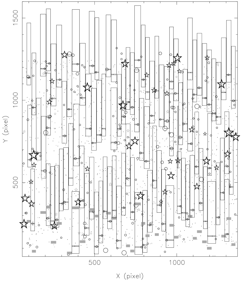
Figure 4: A schematic map of a typical mask design: mask B for the field CNOC 0223+00b5. Objects from the photometric catalog are denoted by circles (galaxies) and stars (stars) with their sizes indicating relative magnitudes. Slit positions are marked with small horizontal rectangles, while the vertical boxes indicate the positions of the spectra. The solid gray boxes mark the positions of the zeroth order contamination. There are a total of 95 slits on this mask.

A typical mask design is shown in Figure 4. In Figures 5 and 6, we show the magnitude distribution and fraction of objects selected as a function of magnitude for masks A and B for the fields in the Patch CNOC 0223+00. Note that bright galaxies have a higher sampling rate relative to the fainter galaxies. This is part of the design philosophy, as the smaller total number of bright galaxies requires a higher sampling rate to provide sufficient statistics.

Figure 3 also presents the pair fraction as a function of separation for objects in the A masks (dot-dashed line) and in the A and B masks (dashed line) for the whole survey, summed field by field, demonstrating the corrective action of having two masks. Note that the two-mask and pair-compensation procedures are still not sufficient to completely correct the lower sampling rate at separations up to about 100^′′. This is simply due to the fact that with only two masks, high galaxy density regions will always be undersampled. Furthermore, at small angles, close triples will be severely undersampled in a two-mask system. The better-than-expected coverage at the smallest angular bin ($<3^{\prime\prime}$) is due to serendipitous observations of very close doubles in a single slit. At large separations ($>300^{\prime\prime}$), the pair fraction is oversampled. This is due to the edge effect of objects near the North/South edges having a higher probability of being placed. Also plotted in Figure 3 (thick solid line) is the pair distribution of the final redshift sample, which follows the mask pair distribution except at large radii, showing a significant drop despite more objects being sampled by the masks at these separations. This drop is due to the poorer image quality at the edges and corners of MOS. The undersampling effect at the arcminute scale is partially corrected by applying a geometric weight (see Section 5) to each object. Nevertheless the redshift sample pair distribution from an entire patch shows periodic spatial features at an amplitude of about 10 to 20% with a period of about the width of the fields($\sim 550^{\prime\prime}$) in the East-West direction. These features are noticeable in the E-W direction but not in the N-S direction due to the fact that extra objects are sampled by the masks at the North/South edges, but not the East/West edges.

Figure 5: The magnitude distribution for objects selected by the mask design algorithm for the A masks (solid histogram) and B masks (dashed histogram) for Patch CNOC 0223+00.

Figure 6: The fraction of objects as a function of magnitude selected by the mask design algorithm for the A masks (solid line), B masks (dot-dashed line) and either mask (heavy dashed line) for the fields in Patch CNOC 0223+00. The fraction for either mask is not identical to the sum of masks A and B due to redundant selections.

3 Photometric Data Reduction

3.1 Photometry

Photometric reduction is performed using the program PPP (Yee, 1991) as described in YEC. Detailed descriptions of object finding, star-galaxy classification, and “total” photometry via growth curve analysis can be found in YEC and Yee (1991).

The photometric catalog in 5 filters is produced using a master object list created from the $R$ image. Although in principle, this procedure will miss extremely blue objects, or red objects in $R-I$; in practice, such an effect is not expected to be significant, since the $R$ band image is by far the deepest in the set. Visual inspection of the images from the other filters indicates that at worst only the occasional very faint blue object is missed, and the $R$-selected catalog (which is 100% complete up to about 23.2 mag) should be complete for objects redder than the extreme color of $B-R=-0.7$ at the $B=22.5$ limit of the primary spectroscopic sample. We note that the photometric catalog contains no objects as blue as $B-R=0.0$, well above the cut-off limit. However, it is clear that these catalogs should not be used to search for $R$-band drop-outs!

The object list is visually inspected, and spurious objects arising from cosmetic defects such as bleeding columns and diffraction spikes, and small structures (e.g., HII regions) within large, well-resolved, low-redshift galaxies are removed. We also pay close attention to close doubles that are missed by the object finding routine, and manually add these to the list. This adjustment is important in preventing stars with a close companion from being misclassified as galaxies.

Because of the slightly different distortion from the optics of the focal reducer of MOS over the large wavelength region covered by the 5 filters, and the fact that three different CCDs with different scales have been used, the master list of objects from the $R$ image is corrected to the co-ordinate system of the other filters via a geometric transformation determined by comparing positions of bright objects in the images.

The photometry from the longer exposure $U$ band images suffers significantly more severely from cosmic-ray hits than the other bands. This is due to both the longer exposure time and the much lower relative flux of the desired signals. Hence, a cosmic-ray detection removal algorithm (as part of the PPP package) is applied to all the $U$ band images before photometry is done. This algorithm detects cosmic-ray hits by first identifying all pixels that are more than 9$\sigma$ above the local sky root-mean-squared fluctuation. These pixels are then tested to see if they are consistent with being part of a real object via a sharpness test. If they are not, they are tagged as cosmic ray detections, and a padding of an additional layer of pixels around them is applied to mask any residual lower level extension of the detection. This simple algorithm works extremely well, and does not accidentally tag any real object pixels. The tagged pixels are then “fixed” by simple linear interpolation. It is found that by applying this algorithm, the $U$ band photometry improves for about 5% of the galaxies based on improved SED fits for objects in the redshift sample.

We note that the photometry catalogs created at the summit in real time (in $R$ and $B$ only) which are used for designing the masks are preliminary. These catalogs are updated later with a more careful inspection and adjustment of the star-galaxy classification parameters. Hence, there are small improvements in the final catalogs compared to the summit catalogs. In general, the final catalogs feature fewer spurious objects, fewer missed closed neighbors, and more reliable the star-galaxy classifications (see Section 3.2), especially for objects situated near edges and corners of the image where the defocusing is significant. However, because the mask design uses the summit catalogs, a number of stars misclassified as galaxies are unwittingly selected for spectroscopic observation. Typically these stars are either near corners or edges, or have a faint, close neighbor. Some of these misclassified objects are active galaxies and quasars; they are discussed in Hall et al. (2000).

The calibration to standard systems is achieved using three to four Landolt (1994) standard fields, plus M67 whenever possible, per each run in the 5 filters. It is found that the calibration of the $g$ band photometry requires a rather large and uncertain color term. This is due to the fact that the $g$ filter used is actually significantly redder than the original $g$ band definition (Thuan & Gunn 1976), and that there are only a small number of standard stars available (compared to the Landolt system). Hence, we have calibrated these images to the $V$ system based on Landolt standards. This results in a smaller color term and in general more stable results. Nevertheless, for completeness we also produce catalogs with the red and the green filters calibrated to the Gunn $r$ and $g$ system. Typical systematic uncertainties in the zero point calibration constants are 0.04, 0.04, 0.05, 0.05, 0.07 for $IRVBU$. Most of the data are obtained under photometric conditions. Small adjustments to compensate for field-to-field differences are made using newly obtained large format CCD images (KPNO 0.9m MOSAIC camera and CFH12K camera) and using the overlapping regions between adjacent fields. While this does not eliminate the systematic uncertainties, it does put every field in a single patch on a consistent calibration.

The final “total” $R$ magnitude for each object is created using the following algorithm. The magnitude from the adopted optimal aperture determined from the $R$-band growth curve (see Yee 1991) is used as the primary magnitude for an object. If the aperture is smaller than $12^{\prime\prime}$, the magnitude is extrapolated to the $12^{\prime\prime}$ aperture by using the stellar PSF shape. This nominally produces a correction of less than 0.05 mag. This procedure provides an exact correction for faint stars, and a first order correction for faint galaxies to compensate for seeing smearing. For galaxies brighter than about 19 mag, a second pass for the growth curve is performed using a maximum aperture size of $24^{\prime\prime}$. The few very bright galaxies ($R\lower 0.43057pt\hbox{\hbox to0.0pt{\raise 2.58334pt\hbox{\hskip 1.29167pt{{$\scriptscriptstyle<$}}}\hss} \kern-1.72218pt{{$\scriptscriptstyle\sim$}}}13.5$) are typically larger than this aperture and their magnitudes can be underestimated by 0.1 to 0.2 magnitudes. The x-y position and star-galaxy classification for each object are also adopted from the $R$ image.

To derive the object magnitude for another filter, we use the color of the object relative to a reference filter. A default color aperture, which is the largest aperture used for color determination between a pair of filters, is set at a relatively large value of 4^′′ to account for the non-uniform PSF in the MOS image. The color between the two filters is formed using the flux inside a color aperture which is the minimum of the adopted optimal apertures for the two filters and the default color aperture. Note that the adopted color aperture radius in general is not a specific aperture used in the tabulated growth curve (which uses apertures with integral pixel diameters). The magnitudes within the color aperture are derived by interpolation of the quantized growth curve. The total magnitude for the filter in question is then the difference between the optimal magnitude for the reference filter, which is nominally chosen to be $R$, and the color. For the $U$ band, the color is formed using $B$ and $U$ to avoid using the long baseline between $R$ and $U$ which may increase the uncertainty. This method of determining the “total magnitude” in each filter has the advantage of always having colors defined from the same aperture for the two filters, and also decreasing the uncertainty in the flux measurement of the fainter filter. However, it does make the assumption that there is a negligible color gradient in the object. The photometry uncertainties for each filter in the color pair at the adopted color aperture are recorded, and the uncertainty of the color is the quadrature sum of the two.

The positions of objects on the CCD frame are determined using an iterative intensity centroid method (see Yee 1991). The uncertainty ranges from better than 0.01 pixels for bright objects to about a pixel for objects near the 5$\sigma$ detection limit. However, the major uncertainty in the relative positions of objects from the same field arises from the pincushion distortion of the focal-reduced image, which could be as large as 5 to 6 pixels at the corners. The distortion is corrected using an image taken through a mask with a grid of pinholes of known separations. In general, the relative positions of objects near the edges and corners may be uncertain systematically up to 1^′′. The star cluster M67 is used as the astrometry reference (Girardi et al. 1989) for determining the scale and rotation of the CCD set-up, to an accuracy of about 0.0004 and 0.05^o, respectively. Note that these uncertainties compound the inaccuracy of the absolute position determinations of objects over the large distances spanned by the fields.

3.2 Star-Galaxy Classification

Star-galaxy classification for the MOS imaging data is particularly challenging due to the large variation in the image quality due to the focal reducer optics. The focus variation across the field is often sufficient to produce crescent- or even donut-shaped PSFs at the corners. We adopt the observational procedure of performing focusing consistently at the same predetermined region about 1/3 of the way outwards from the center of the CCD, so that within the defined area the image quality variation is minimized. A variable PSF classification scheme, as outlined in YEC, is used. This procedure essentially compares the growth curve shape of each object with the four nearest PSF standards, one in each quadrant centered on the object (see Yee 1991 and YEC). The PSF standards are chosen automatically; however, manual intervention in the choices of PSFs is often required near the corners and edges of the image. Typically 20 to 40 reference PSFs are used per field.

Stars having a very close neighbor of either a galaxy or another star are occasionally misclassified as non-stellar. These misclassifications are corrected by hand during visual inspection of the classifier plot. In general, objects down to a brightness of $R\sim 22$ mag have robust star-galaxy classification, beyond which some faint galaxies begin to merge into the stellar sequence (e.g., see Figure 2 in YEC). A statistical variable star-galaxy classification criterion is used for the faint objects (see Yee 1991) to compensate for the merging of the star and galaxy sequences in the classifier space. While the separation between stars and galaxies is excellent at magnitudes brighter than the nominal spectroscopic limit of $R=21.5$, quasars, luminous distant active galactic nuclei, and a small number of compact galaxies may be missed in the spectroscopic sample. A more detailed discussion of the effect of star-galaxy classification on compact extragalactic objects is provided in Hall et al. (2000) which analyses the sample of serendipitous AGN and quasars in the CNOC2 sample,

4 Spectroscopic Reduction

4.1 Spectral Extraction

The spectrum of each object is extracted and wavelength and flux calibrated using semiautomated IRAF reduction procedures. Many of the procedures are the same as those used for the CNOC1 survey as described in Section 6.2 of Yee, Ellingson & Carlberg (1996). Here we summarize those procedures and discuss in detail only those changes made for CNOC2. The scripts and programs used are available from G. Wirth (wirth@keck.hawaii.edu). A major conceptual change is that instead of extracting all the spectra from the same large image, each individual spectrum is copied to a smaller subimage upon which the extraction is performed.

Each mask has a flatfield and arc lamp image and typically two individual spectroscopic exposures. The individual spectroscopic exposures are cleaned of cosmic rays (see YEC), overscan subtracted and summed after applying small shifts to correct for flexure in a handful of cases. Regions of zero-order contamination are interpolated over on the flatfield after being marked interactively.

Since the relative position of each spectrum on the CCD is known exactly in advance, for each mask it is easy to construct an automatic extraction file containing the spatial and dispersion position of the objects and the relative positions of the edges of each slit. The automatic extraction file is used to create an IRAF aperture database containing the aperture position, width, and sky background ranges for each object, including serendipitous objects not targeted in the mask design. Three subimages are then created for each object by copying the same region from the summed spectroscopic exposure, flatfield image, and arc lamp image. Each flatfield subimage is normalized using a cubic spline fit to the mean flat field wavelength profile, leaving only pixel-to-pixel variations. The resulting response subimage is divided into the object subimage to yield a flattened object subimage.

Each object subimage is interactively examined and the default object and background apertures adjusted if necessary. Notes are made at this stage of any salient features of the spectrum, including emission line(s), a very faint or invisible continuum, overlapping spectra, multiple objects per slit, etc. The spectrum is then extracted using variance weighting and an arc spectrum is extracted from the arc lamp subimage using the same extraction aperture and profile weighting. The arc lamp images contain lines from He, Ne and Ar, and give 11 lines strong enough and sufficiently unblended to be used for wavelength calibration. There is a gap with no arc lines between 5015Å and 5875Å  where the wavelength calibration is less certain. The wavelength calibration solution for each subimage is found by interactively identifying several arc lines, using a line database to identify the rest, and then fitting a cubic polynomial to the data. The resulting wavelength solution is non-linear (with deviations of over 10Å from linear). Typical rms residuals to the fit for the 11 arc lines are less than 0.1Å. The wavelength solution changes significantly for spectra at differing locations on the CCD, with the mean dispersion ranging from 4.9Å per pixel at the bottom to 5.1Å per pixel at the top (for the STIS2 CCD). The object spectra are wavelength calibrated, and all linearized to run from 4390Å to 6292.21Å with a uniform dispersion of 4.89Å/pixel. The wavelength solutions are checked by visual inspection of the wavelengths of the bright sky lines. The data are then extinction corrected and flux calibrated to $F_{\lambda}$. The flux calibration uses observations of standard stars, generally taken through one of the central apertures. Using these stars, the end-to-end throughput (photons hitting the telescope primary, through to electrons detected by the CCD) for the typical seeing is fairly flat across the blocking filter bandpass, with measured values between 10 and 15%. Slits near the corners of the mask suffer from significant vignetting, which has not been corrected for in the current data. As with CNOC1, the relative flux calibration should be considered accurate to $\lesssim 20$% across large wavelength ranges. The absolute flux calibration of the spectra is considerably more uncertain.

Regions 45Å wide around the bright night sky emission lines at 5577Å and 5892Å are automatically interpolated over. Finally, the spectra are examined and residual cosmic rays or other bad regions are interactively marked and interpolated over, including regions 125Å wide around zero order contamination. These interpolated spectra are the final versions used for redshift determination, but we also found it advantageous to keep copies of the uninterpolated spectra to help confirm redshifts where a feature falls within an interpolated region. A total of 14932 spectra were extracted during the course of the CNOC2 data analysis.

4.2 Cross-Correlations

We determine redshifts using the cross-correlation technique described by YEC ( see also Ellingson & Yee 1994). Our method is similar to standard techniques (e.g., Tonry & Davis 1979), except for a second calculation of the cross-correlation function, which is used to remove biases resulting from the large redshift range we need to consider ($0<z\lesssim 0.7$), coupled with the finite spectral coverage of both our object and template spectra. The reader is referred to YEC for details.

The object spectra are cross-correlated against three galaxy templates, specifically elliptical, Sbc, and Scd galaxy spectra taken from the spectrophotometric galaxy atlas of Kennicutt (1992). All object spectra, along with their associated cross-correlation functions against each template, are visually inspected to verify or reject the redshifts first determined automatically by the cross-correlation program on the basis of the values of the cross-correlation coefficient $R_{cor}$ and peak heights (Tonry & Davis 1979). Generally the redshift corresponding to the template with the highest $R_{cor}$ value is adopted, but occasionally a template with a somewhat lower $R_{cor}$ value may be chosen if visual inspection deems it a better spectral match to the object galaxy. Low signal-to-noise spectra with indeterminable or uncertain redshifts, typically with $R_{cor}\lesssim 3$, are rejected. Figure 7 shows example spectra and cross-correlation functions for galaxies of different spectral types and different $R_{cor}$ values. We assign the galaxy spectral type, denoted “Scl,” according to the cross-correlation template chosen, where Scl=2, 4, and 5 correspond to the elliptical, Sbc, and Scd templates, respectively. The visual inspection also includes examination of the two-dimensional spectral images, both before and after cosmic ray removal, which allows us to reject any remaining cosmic rays that might otherwise masquerade as emission lines in the extracted one-dimensional spectra. Contaminating stellar spectra, as well as unusual spectra (e.g., AGN or spectroscopic gravitational lens candidates, see Hall et al. 2000) are also identified during the visual inspection process. Objects classified as AGN or QSO are designated as Scl=6. In addition, objects without assigned redshifts but with spectra of signal-to-noise ratios judged sufficient to have detected spectral features if they were present are flagged and denoted by Scl=88. Spectroscopically identified stars are designated as Scl=77. The IRAF add-on radial velocity package RVSAO (Kurtz & Mink 1998) is used to aid in graphical display and visual redshift assessment of our spectra.

4.3 Redshift Verification and Uncertainty

The redshifts determined during the “first pass” visual inspection described above are subjected to confirmation in several subsequent steps. A “second pass” visual inspection of those spectra assigned a first-pass redshift is made to verify the original redshift determination and to flag problem cases for final inspection. This is done by one of us (H. Lin) on the spectra in bulk, after all the survey data has been acquired and all first-pass inspections completed, in order to provide a single reasonably uniform categorization of the redshift quality. During second-pass inspection, the original first-pass redshifts are assigned to three categories: good, probable, and questionable/bad. Questionable/bad redshifts are subjected to a final visual inspection, as described below. Note this questionable/bad category also includes cases where a clerical mistake was made during first pass on an otherwise obviously good redshift. For probable redshifts, we apply an additional, more objective photometric-redshift (photo-$z$) verification test to confirm the redshift or to flag the spectrum for final visual inspection.

The photo-$z$ calibration is done using the empirical polynomial fitting method of Connolly et al. (1995). Separate fits are determined for Scl=2, 4, and 5 galaxies, using the full 4-patch CNOC2 data set, but the calibration sample is restricted to those galaxies with second-pass “good” redshifts and high cross-correlation $R_{cor}$ values ($\geq 6$ for Scl=2,4; $\geq 12$ for Scl=5). For Scl=2 and 4 objects, the fits include up to linear-order terms in in the $U\!BV\!RI$ magnitudes, but for Scl=5, we also include terms up to quadratic order to improve the fit. We take out any redshift-dependent residuals in our photo-$z$ fit by subtracting the median difference between photometric and spectroscopic redshift, in bins of width $\Delta z=0.1$ in spectroscopic redshift. Note that since we are interested in checking the consistency between photometric and spectroscopic redshifts, rather than trying to derive photo-$z$’s for objects with no spectroscopy in the first place, it is entirely valid to use existing spectroscopic redshift and spectral class (Scl) information to optimize the photo-$z$ fits. Using the calibration sample of second-pass good redshifts, we find that only about 10% of these galaxies have $|z({\rm photometric})-z({\rm spectroscopic})|>0.065$, 0.09, or 0.15 for Scl=2, 4, or 5, respectively. We then adopt these simple cuts to flag for final inspection those second-pass probable redshifts which show a large discrepancy with their respective photometric redshift estimates.

The third and final pass is then carried out by two of us (P. Hall, H. Lin), on the following objects: those with second-pass questionable/bad redshifts, those with second-pass probable redshifts failing the photo-$z$ verification test, those with $R_{cor}<4$, those morphologically classified as galaxies or probable galaxies but spectroscopically classified as stars (and vice versa), and all objects which were not initially assigned redshifts but which do have spectra of reasonable signal-to-noise ratios (i.e., Scl=88). Redshifts for which both inspectors agree are good (bad) are retained (rejected); those for which the inspectors disagree are resolved by a tie-breaking vote cast by a third person (H. Yee). We also correct any obvious mistakes in the redshift at this point (e.g., a redshift based on a [OIII]$\lambda\lambda$5007 emission line that was mistakenly or accidentally taken to be a [OII]$\lambda$3727 line during first pass). As an example, overall about 250 redshifts out of $\sim$1550 (i.e., $\sim 15$%) from the 0223+00 patch are third-pass inspected and 36 of these are ultimately excluded from the final redshift catalog. Thus, the final catalog contains objects that have secure redshifts with their quality approximately ranked by the correlation $R_{cor}$ values.

Finally, we use redundant redshift measurements, typically from independent pairs of A and B mask spectra, to empirically calibrate the redshift errors calculated by our cross-correlation program. Specifically, we examine the distribution of velocity differences for the redundant pairs, appropriately normalized by the quadrature sum of the formal velocity errors returned by the program. We find that the original program errors need to be multiplied by a factor of 1.3 in order to match the empirical velocity differences, but once that is done a K-S test shows that the resulting normalized velocity difference distribution is indeed consistent with a Gaussian. In Figure 8 we plot the velocity difference distribution for the 303 redundant pairs in the 0223+00 patch; the rms velocity difference, divided by $\sqrt{2}$, is 103 km s^-1, which indicates our typical random velocity error on a single redshift measurement. We estimate the systematic error in the velocity zero point for our templates to be approximately 30 km s^-1, as detailed in YEC.

Figure 8: The distribution of velocity differences for redundant $z$ measurements from the CNOC 0223+00 patch scaled by $\sqrt{2}$. The distribution has a dispersion of 103 km s^-1.

5 Completeness and Weights

The practical difficulty of obtaining spectroscopic observations for every single galaxy in a faint galaxy sample requires such a survey to adopt a sparse sampling strategy. In the case of the CNOC2 survey, the sampling is slightly under 2 to 1; and the sampling itself is not necessarily uniform. For example, objects near the edges in the spectral direction, and objects in low galaxy density regions are more likely to be sampled simply due to geometric considerations. Furthermore, the success rate of obtaining a redshift when a galaxy spectrum is obtained depends on many factors, the foremost being the signal-to-noise ratio and the strength of the spectral features. For some galaxies, because of the relatively short spectrum, there may not be any useful identification features for deriving a robust redshift. Hence, to convert an observed redshift sample to a complete sample requires a detailed understanding of the various effects and methods of accounting for them. For the CNOC1 Cluster Redshift Survey, YEC described in detail their method of compensating for these various factors by attaching a series of statistical weights to each galaxy. The CNOC2 survey uses the same method to assign weights to each galaxy in the redshift sample. Here, we will describe very briefly the determination of weights, with emphasis on the small variations from the method used by YEC.

For each galaxy, a selection function $S=S_{m}S_{xy}S_{c}S_{z}$ is computed, where $S_{m}(m)$ is the magnitude ($m$) selection function, $S_{xy}(x,y,m)$ is the geometric selection function based on the location ($x,y$) of the object, $S_{c}(c,m)$ is the color ($c$) selection function, and $S_{z}(z,m)$ is the redshift selection function. The weight, $W$, for each galaxy is then $1/S$. $S_{m}$ is chosen as the primary selection function which has a value between 0 and 1; whereas the other selection functions are considered as modifiers to $S_{m}$ and are normalized to have a mean over the sample of $\sim 1.0$ (with the exception of $S_{z}$). This description of the weights of the galaxies allows one to omit any of the secondary selection functions if they are deemed unnecessary for the analysis.

Selection functions are computed for each filter for every object with a redshift. $S_{m}$ is derived by counting galaxies in a running bin of $\pm$0.25 magnitudes around each object, taking the ratio of the number with redshifts to that in the photometric sample. Examples of the magnitude selection function for individual fields are shown in Figure 9 for the patch CNOC 0223+00. Because there are significant variations of coverage from field to field due to observing conditions and object density – the nominal 20% selection limit (i.e., $S_{m}=0.2$) varies from $R_{c}=21.1$ to 21.8 mag – the magnitude selection function is computed in individual fields rather than over the whole patch (which was done in the CNOC1 catalogs, which have many fewer fields per cluster). This is equivalent to applying a large geometric filter to the magnitude selection function. Variations over smaller angular scale are corrected by $S_{xy}$, which is computed by counting galaxies within $\pm$0.5 mag over an area of 2.0 arcminutes around the object. The color selection function is similarly accomplished by counting galaxies over a color range of $\pm$0.25 mag. The colors used for $I$, $R$, $V$, $B$, and $U$ are $R-I$, $B-R$, $V-R$, $B-R$, and $U-B$, respectively.

Figure 9: Magnitude selection function for the fields in the CNOC 0223+00 patch. Each point represents the magnitude selection value, $S_{m}$, for the $R$ band of an object. The thick solid line represents the mean magnitude selection function for the whole patch computed in 1/2 mag bins. The fluctuations at the bright magnitudes are due to small number statistics. To illustrate the variations amongst the fields, the points from the galaxies in fields a2 and c4 are plotted as open circles and triangles, respectively. The field a2 has a particularly low selection for $R<20.5$ mag galaxies due in part to the relatively poor observing conditions for mask A; while the field c4 is more representative.

The calculations of $S_{m}$, $S_{xy}$, and $S_{c}$ are all performed strictly empirically using the galaxy catalog, and they can be easily recomputed with different bin sizes, sampling areas, or reference colors. However, the computation of $S_{z}$ is model dependent, as it requires an estimate of the number of galaxies of a certain magnitude and color which are outside the measurable redshift range. This requires knowledge of the luminosity function of galaxies as a function of color and redshift, which is in fact one of the goals in the study of galaxy evolution. If the LF of the galaxies is known, then a simple correction to $S_{m}$, the magnitude selection function, is $f_{z}(z1,z2)/f_{LF}(z1,z2)$; where $f_{z}(z1,z2)$ is the fraction of galaxies in the redshift sample between $z1$ and $z2$, and $f_{LF}(z1,z2)$ is the fraction of galaxies in the same $z$ range as modeled by the LF. Using the LF derived by Lin et al. (1999) from two of the 4 CNOC patches, we can estimate the redshift selection function, $S_{z}$, as a function of magnitude. We note that Lin et al. derived the LF using a different redshift weight correction based on colors of galaxies, although the LF and $S_{z}$ can be derived iteratively using the above method for determining $S_{z}$. As an example, Table 4 lists $W_{z}$ derived based on count models in half magnitude bins for the patch CNOC 0223+00. The correction to $W_{m}$ due to the redshift range effect is significant at $R\lower 0.43057pt\hbox{\hbox to0.0pt{\raise 2.58334pt\hbox{\hskip 1.29167pt{{$\scriptscriptstyle>$}}}\hss} \kern-1.72218pt{{$\scriptscriptstyle\sim$}}}20.5$, rising to as much as 30% at the nominal spectroscopic sample limit of $R=21.5$. A large correction is expected at the faint end, as fainter galaxies have a higher mean redshift, resulting in fewer galaxies having their redshift measured. Values of $W_{z}$ for individual objects in the catalogs are derived by interpolating the results from binned data. Because of the near 100% success rate and small number statistics at bright magnitudes, $W_{z}$ is fixed at 1.0 at $R<18.0$.

Another independent method for accurately accounting for the redshift selection effect is to compare the redshift sample to a photometric redshift sample derived from the 5 color photometric data. This method will be discussed in a future paper.

Figure 11: The photometric sample of the CNOC 0223+00 patch. All galaxies brighter than 23.0 mag in $R$ (which is 100% complete) are plotted.

6 The Data Catalog for the Patch CNOC 0223+00

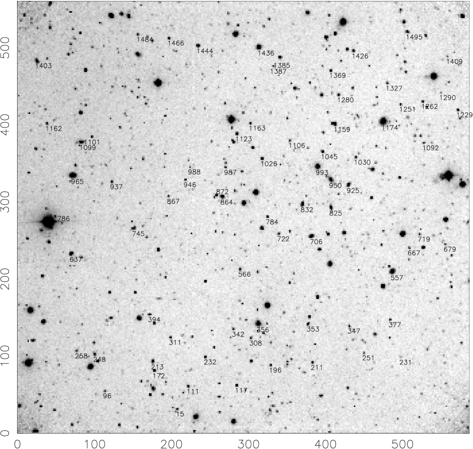
Figure 10: An example of single field $R$-band images from the survey plotted as gray scales. The field is CNOC 0223+00b5. North-East is upper left, with the axes marked in 100 arcsecond intervals. The total field size is $\sim 10^{\prime}\times 10^{\prime}$. The PPP object numbers of objects with measured redshifts are shown. (Note: This version of the image has been block averaged to reduce the file size.)

The patch CNOC 0223+00 contains 19 fields. An example of a $R$ MOS image of a single field is shown as a gray scale plot in Figure 10, with objects having measured redshifts marked. The layout of the 19 fields of the patch is presented in Figure 11, with all galaxies brighter than $R=23.0$ (100% complete) marked. The total area in the defined region for the patch is 1408.7 square arcminutes. The patch contains to this limit 9554 objects classified as galaxies and 2574 classified as stars. The sky and redshift distributions of the redshift sample are shown in Figures 12 and 13. A total of 1541 redshifts are measured from 3820 spectrum (with a redundancy rate of 32.9%). The number of galaxies with $R\leq 21.5$ is 2692, of which 1293 have a measured redshift. The cumulative sampling rate at $R=21.5$ is 48.0%, with a raw success rate of 67.3%. Figure 9 illustrates the differential sampling rate (i.e. $S_{m}$) of individual objects as a function of magnitude. The raw and redshift-selection-corrected success rates as a function of $R$ magnitude are tabulated in Table 4 and plotted in Figure 14. The corrected success rate is close to 100% for galaxies brighter than 20.0, and close to 70% at the nominal primary spectroscopy limit of $R=21.5$. We note that the success rates tabulated reflect the sum of the A and B masks, with the A masks having half the exposure time of that of the B masks. Typical spectra and their correlation functions are plotted in Figure 7. Figure 8 illustrates the histogram of $\Delta v$ from redundant spectroscopic observations. The distribution produces an estimate of the average uncertainty for the redshift measurements of 103 km s^-1.

Figure 12: Same as Figure 12, but for the redshift sample with $R<21.5$ mag. The size of the circles is proportional to the apparent $R$ magnitude of the galaxies.

Some statistics for each field are presented in Table 5. These include the $5\sigma$ detection limits for the $R$ and $B$ filters. These are fiducial limits determined using stellar PSFs; typical 100% completeness for galaxies are 0.6 to 0.8 mag brighter (see Yee 1991). The numbers in brackets indicate the runs (and hence the CCD used, see Table 2) from which the $R$ and $B$ images were obtained. The mean $5\sigma$ magnitude limits are $23.87\pm 0.13$ and $24.49\pm 0.13$ for $R$ and $B$, respectively, where the uncertainty is the rms width of the distribution. The 100% photometric completeness limit is approximately 0.7 to 0.9 magnitudes brighter than the $5\sigma$ limit (see Yee 1991). For the other 3 filters: $I$, $V$, and $U$, the mean 5$\sigma$ magnitude limits are 22.80$\pm$0.22, 24.09$\pm$0.12, and 23.04$\pm$0.15, respectively. Also listed in Table 5 are the number of redshifts measured in each field, with the bracketed numbers indicating the runs from which masks A, B, and C were obtained. The integrated selection function $S_{m}$ at $R=21.5$ and the differential selection rate at $21.0<R<21.5$ are also shown in Table 5. These numbers provide an idea of the variations from field to field expected in a patch.

Figure 14: The raw success rate (solid line) and the redshift-selection corrected success rate (dashed line) for the CNOC 0223+00 patch.

The fields are merged into a patch by matching a reference object which appears in both adjacent fields. Table 6 is a sample catalog for the patch CNOC 0223+00 which contains every 25th galaxy with redshifts from the full catalog to demonstrate some of the information tabulated for each object in the full catalog. Listed in the sample catalog are the following columns:

Column 1: the PPP object number – the first two digits represent the field number, while the last 4 digits is the sequential object number within the field ordered from South to North.

Column 2: the offset in RA in arc seconds from the fiducial origin in the a0 field with West being positive.

Column 3: the offset in Dec in arc seconds with North being positive. The object positions, both $\Delta$RA and $\Delta$Dec, have not been put on a proper astrometric grid. The relative position between two objects are in general accurate to 1 to 2 ^′′ within the same field, and could be uncertain by as much as 5^′′ or more across the patch (see Section 3.1).

Columns 4 to 8 : the $I$, $R$, $V$, $B$, and $U$ magnitudes. The photometric uncertainties for $R$ and $B$ are shown to illustrate the typical errors. The errors are tabulated in 1/100 magnitude units. Note that a 0.03 mag “aperture” uncertainty is added in quadrature to the photon noise error for all objects. This accounts for the uncertainty in determining the optimal aperture for the object (See YEC).

Column 9: the redshift and uncertainty. The uncertainty has been scaled by the empirically determined 1.3 factor from that produced by the cross-correlation algorithm (see Section 4.3) and is tabulated in units of 0.00001 in redshift.

Column 10: the spectroscopic classification, with 2=elliptical spectrum, 4=intermediate-type spectrum, 5=emission-line spectrum, 6=active galactic nuclei.

Column 11: cross-correlation coefficient value ($R_{cor}$).

Column 12: Spectral energy distribution (SED) class determined by fitting the 5 color photometry to the empirical SEDs of galaxies of different spectral types from Coleman, Wu, & Weedman (1980). The template SEDs of E/S0, Sbc, Scd, and Im classes from Coleman, Wu, & Weedman are designated as 0.0, 1.0, 2.0, and 3.0. An additional very blue template, denoted as 4.0, is created from the GISSEL library (Bruzual & Charlot 1996) for modeling late-type strongly star-forming galaxies. Intermediate SED classes are interpolations of these templates.

Column 13: k-correction for the filter $R$ determined using the SED class fit and spectral model.

Column 14: magnitude weight for the filter $R$.

In the full electronic version of the catalog, the color aperture error, the k-correction and the magnitude, geometric, and color weights for the remaining 4 filters, and the redshift weight for each object are also listed. The central position in RA and Dec of the catalog (i.e., $\Delta$RA=0.0 and $\Delta$Dec=0.0) is 00:23:29.2, +00:05:14 (1950). The complete catalog and detailed explanatory notes for the catalog can be found in a number of websites: http://adc.gsfc.nasa.gov/, http://www.astro.utoronto.ca/$\sim$hyee/CNOC2/, and http://cadcwww.hia.nrc.ca.

Also available electronically is a ”field-area map”, which is a two-dimensional array containing 0’s and 1’s, mapping the sampled area of the patch with a 2^′′/pixel resolution. This map allows the determination of the exact area on the sky covered, including the effect of blockage by bright stars.

Table 1: CNOC2 Redshift Survey Patches

Name	RA	Dec	$b$	$E(B-V)$	No. of Fields	Total Area	No. of Masks
CNOC 0223+00	02 23 30.0	+00 06 06	–54.3	.036	19	1408.7	39
CNOC 0920+37	09 20 40.7	+37 18 17	+45.6	.012	19	1366.9	40
CNOC 1447+09	14 47 11.6	+09 21 21	+57.2	.029	17	1240.0	34
CNOC 2148–05	21 48 43.0	–05 47 32	–41.6	.035	19	1417.9	39

Table 2: Properties of CCD Detectors and Exposure Times

	ORBIT1	LORAL3	STIS2
Pixel size ($\mu$m)	15	15	21
Pixel scale (′′)	0.313	0.313	0.438
Imaging Area Used (pixels)	$2048\times 2048$	$2048\times 2048$	$1416\times 1368$
Defined Field Area (′)	$7.3\times 9.2$	$7.3\times 9.2$	$8.3\times 9.2$
Å per pixel	3.55	3.55	4.96
Spectroscopy Exp. Time (sec)
Mask A	$\sim$3000	$\sim$3600	2400
Mask B	$\sim$7000	$\sim$7200	4800
Imaging Exp. Time (sec)
Filter $I_{c}$	420	600	360
Filter $R_{c}$	420	600	420
Filter $V$	420	600	420
Filter $B$	420	900	480
Filter $U$	not used	not used	900

Table 3: Journal of Observations

Run Number	Beginning Date (UT)	Number of Nights	CCD
1.	1995/02/27	8	ORBIT1
2.	1995/10/20	8	LORAL3
3.	1996/02/13	9	LORAL3
4.	1996/10/11	8	STIS2
5.	1997/02/04	8	STIS2
6.	1997/08/30	6	STIS2
7.	1998/05/23	6	STIS2

Table 4: Redshift Selection Function and Success Rates for Patch CNOC 0223+00

Mag bin	$f_{z}(0.12,0.55)$	$f_{LF}(0.12,0.55)$	$W_{z}$	Raw Success Rate	Corrected Success Rate
17.0–17.5	0.667	0.500	0.752	1.00	1.33
17.5–18.0	0.923	0.687	0.746	0.87	1.16
18.0–18.5	0.854	0.814	0.953	0.92	0.97
18.5–19.0	0.970	0.887	0.915	0.91	0.99
19.0–19.5	0.928	0.927	0.999	0.88	0.88
19.5–20.0	0.950	0.927	0.976	0.85	0.87
20.0–20.5	0.942	0.869	0.922	0.77	0.84
20.5–21.0	0.903	0.752	0.833	0.63	0.76
21.0–21.5	0.853	0.608	0.713	0.49	0.69
21.5–22.0	0.774	0.472	0.610	0.36	0.59

Table 5: Statistics for Patch CNOC 0223+00

Field Number	Field Name	$R_{c}$	$B$	$N_{z}$	$S_{R<21.5}$	$S_{21.0<R<21.5}$
1	a0	24.02 (2)	24.55 (4)	55 (2,2,4)	0.399	0.260
2	a1	24.02 (2)	24.35 (4)	62 (2,2)	0.512	0.327
3	a2	24.04 (2)	24.56 (4)	70 (2,4)	0.424	0.400
4	a3	23.95 (4)	24.60 (4)	57 (2,4)	0.518	0.358
5	a4	23.86 (4)	24.63 (4)	70 (4,4)	0.387	0.164
6	a5	24.02 (4)	24.55 (4)	78 (4,4)	0.382	0.151
7	a6	23.93 (6)	24.57 (6)	88 (6,6)	0.550	0.236
8	b1	23.78 (4)	24.53 (4)	49 (4,4)	0.383	0.255
9	b2	23.64 (4)	24.38 (4)	65 (4,4)	0.489	0.373
10	b3	23.83 (4)	24.17 (4)	60 (4,4)	0.472	0.315
11	b4	23.67 (4)	24.51 (4)	77 (4,4)	0.653	0.475
12	b5	23.78 (4)	24.47 (4)	62 (4,4)	0.508	0.255
13	c1	23.87 (4)	24.59 (4)	87 (4,4)	0.503	0.279
14	c2	23.76 (4)	24.32 (4)	97 (4,4)	0.508	0.293
15	c3	23.63 (4)	24.47 (4)	60 (4,4)	0.492	0.213
16	c4	23.93 (4)	24.60 (4)	64 (5,5)	0.454	0.172
17	c5	23.92 (4)	24.66 (4)	72 (5,5)	0.500	0.151
18	c6	23.90 (4)	24.27 (4)	61 (5,6)	0.535	0.216
19	c7	24.04 (6)	24.46 (6)	59 (6,6)	0.590	0.378
Total				1293	0.480	0.270

Table 6: Sample Catalog for the CNOC 0223+00 Patch

PPP#	$\Delta$ RA	$\Delta$ Dec	$I_{c}$	$R_{c}$	$V$	$B$	$U$	$z$	Scl	$R_{cor}$	SED	K($R_{c}$)	$W_{m}$
062246	16.10	2540.30	13.62	14.25$\pm$03	14.89	15.89$\pm$03	16.22	0.02383$\pm$034	5	4.56	0.20	0.02	1.00
071667	219.00	2918.60	17.21	17.97$\pm$03	18.86	20.59$\pm$04	0.00	0.25109$\pm$029	2	11.10	0.08	0.29	1.25
120965	-208.60	-400.20	17.77	18.28$\pm$03	18.71	19.37$\pm$03	19.43	0.09095$\pm$036	4	3.98	2.02	0.01	1.00
182286	1925.80	-1229.50	17.85	18.50$\pm$03	18.94	19.90$\pm$03	19.63	0.14918$\pm$036	5	4.03	1.49	0.05	1.00
031395	9.50	982.70	18.03	18.73$\pm$03	19.49	20.72$\pm$04	20.54	0.26713$\pm$031	4	6.32	0.66	0.21	1.40
061186	-217.50	2321.70	18.20	18.87$\pm$03	19.47	20.58$\pm$04	20.19	0.23756$\pm$034	4	5.49	1.27	0.10	1.50
170596	871.70	-1589.60	18.24	19.05$\pm$03	20.05	21.56$\pm$04	21.79	0.28857$\pm$039	2	7.98	0.07	0.34	1.09
120706	101.50	-478.90	18.44	19.17$\pm$03	19.97	21.13$\pm$04	21.00	0.35873$\pm$042	4	3.86	0.88	0.25	1.17
172593	1038.20	-1233.90	18.48	19.29$\pm$03	19.96	21.31$\pm$04	21.41	0.27141$\pm$030	5	8.61	0.63	0.23	1.50
020465	198.00	326.80	18.78	19.38$\pm$03	19.83	20.83$\pm$04	20.43	0.25072$\pm$029	5	9.52	2.14	0.00	1.80
130656	758.30	-43.30	18.67	19.49$\pm$03	20.57	22.28$\pm$08	22.91	0.30653$\pm$033	2	6.04	-0.04	0.39	1.40
110674	-244.50	-945.70	18.57	19.60$\pm$03	20.80	22.43$\pm$08	23.40	0.50610$\pm$130	2	7.00	0.27	0.77	1.17
101269	-511.00	-812.60	18.94	19.68$\pm$03	20.56	21.94$\pm$06	22.30	0.23808$\pm$029	2	9.35	0.21	0.25	1.12
072259	228.20	3048.20	18.93	19.75$\pm$04	20.69	22.03$\pm$06	0.00	0.38166$\pm$055	4	3.70	0.57	0.38	1.47
061882	-233.80	2463.40	18.93	19.82$\pm$04	20.92	22.49$\pm$08	23.18	0.34269$\pm$039	2	4.31	0.06	0.45	1.57
121045	115.80	-369.20	19.18	19.88$\pm$04	20.61	21.78$\pm$05	21.63	0.26797$\pm$030	4	7.42	0.79	0.19	1.71
060425	-90.60	2164.80	19.26	19.93$\pm$04	20.73	21.74$\pm$05	21.38	0.39500$\pm$052	4	2.74	1.53	0.17	1.67
140958	731.80	-454.60	19.18	19.98$\pm$04	21.13	22.70$\pm$08	23.38	0.35861$\pm$035	2	5.58	0.23	0.44	1.41
131723	527.80	238.40	19.53	20.02$\pm$04	20.42	21.24$\pm$04	21.03	0.20448$\pm$027	5	11.25	2.52	-0.04	1.35
041010	-80.40	1353.00	19.61	20.09$\pm$04	20.62	21.32$\pm$04	21.16	0.19236$\pm$034	5	5.26	2.28	-0.01	1.27
141131	724.90	-414.70	19.51	20.14$\pm$04	20.98	22.04$\pm$06	21.60	0.40983$\pm$031	5	6.84	1.56	0.17	1.61
191280	2355.00	-1452.90	19.66	20.19$\pm$04	20.77	21.76$\pm$05	21.41	0.34958$\pm$031	5	7.50	2.20	0.03	1.19
062186	3.20	2526.10	19.66	20.23$\pm$05	21.08	22.06$\pm$07	22.75	0.47153$\pm$040	5	4.16	0.98	0.34	2.22
071950	174.10	2978.30	19.43	20.29$\pm$04	21.50	22.90$\pm$11	0.00	0.47065$\pm$038	4	5.26	0.48	0.58	1.16
040918	29.70	1333.40	19.64	20.32$\pm$04	21.27	21.82$\pm$06	21.53	0.57002$\pm$031	5	7.97	2.16	0.23	1.50
090572	-352.60	-491.60	19.70	20.37$\pm$04	21.05	22.11$\pm$06	21.83	0.36132$\pm$030	5	8.19	1.69	0.12	2.27
141456	576.80	-332.70	19.49	20.41$\pm$05	21.68	23.27$\pm$10	24.40	0.43243$\pm$036	2	5.12	0.16	0.61	2.21
172640	1270.80	-1225.90	19.64	20.45$\pm$04	21.14	22.51$\pm$06	22.45	0.30501$\pm$030	5	7.76	0.69	0.25	1.12
120172	-103.10	-653.80	20.03	20.48$\pm$04	20.88	21.69$\pm$05	21.42	0.21864$\pm$027	5	12.80	2.62	-0.05	1.73
160180	1273.00	-1157.20	19.58	20.54$\pm$04	21.57	22.94$\pm$10	23.26	0.38611$\pm$017	5	7.60	0.29	0.48	1.85
081751	-499.30	254.00	19.67	20.58$\pm$04	21.36	23.33$\pm$10	25.75	0.38505$\pm$033	2	6.60	0.25	0.48	3.12
170502	896.60	-1605.40	19.70	20.62$\pm$04	21.91	23.35$\pm$11	24.21	0.38629$\pm$035	2	5.70	0.03	0.55	1.48
172734	1090.10	-1212.20	20.14	20.66$\pm$04	21.32	22.22$\pm$06	21.67	0.44641$\pm$030	5	8.21	2.42	0.04	1.52
061970	118.80	2479.40	20.29	20.70$\pm$04	21.30	22.03$\pm$06	21.67	0.40574$\pm$029	5	10.51	2.67	-0.03	2.67
031433	114.20	989.70	20.33	20.76$\pm$04	21.28	22.19$\pm$06	21.83	0.42381$\pm$031	5	7.71	2.50	0.01	2.37
140585	338.70	-541.00	19.85	20.78$\pm$04	21.95	23.94$\pm$29	23.94	0.44481$\pm$039	2	4.69	0.23	0.62	1.75
131602	494.50	204.30	19.95	20.82$\pm$04	22.03	23.76$\pm$13	24.79	0.50480$\pm$130	1	4.00	0.42	0.69	2.69
110893	-41.40	-868.70	20.03	20.85$\pm$05	21.54	22.60$\pm$08	22.49	0.30240$\pm$013	5	8.64	0.83	0.21	1.87
140073	727.80	-688.20	20.28	20.89$\pm$04	21.67	22.40$\pm$08	21.80	0.61474$\pm$046	5	3.98	2.42	0.21	1.66
150997	560.00	-933.50	20.08	20.93$\pm$04	22.02	23.70$\pm$17	23.79	0.40895$\pm$056	2	2.57	0.36	0.50	2.11
150326	628.80	-1102.70	20.10	20.96$\pm$04	22.09	23.88$\pm$19	26.84	0.38629$\pm$036	2	5.48	0.05	0.54	2.23
131156	718.70	93.30	20.46	21.01$\pm$04	21.77	22.64$\pm$07	22.19	0.39897$\pm$031	5	6.94	2.12	0.07	2.44
140971	361.50	-450.80	20.47	21.05$\pm$05	21.69	22.67$\pm$09	21.96	0.36204$\pm$029	5	10.29	2.20	0.04	2.29
151247	669.30	-859.10	20.47	21.09$\pm$05	21.62	22.43$\pm$07	22.17	0.35917$\pm$027	5	16.01	2.38	0.01	2.30
041846	174.70	1556.40	20.54	21.13$\pm$05	21.73	22.16$\pm$06	21.88	0.52669$\pm$034	5	6.50	3.00	-0.07	2.48
101399	-326.20	-762.70	20.31	21.16$\pm$06	22.27	23.18$\pm$16	22.28	0.58764$\pm$034	5	6.73	1.44	0.43	2.79
040195	87.10	1137.70	20.57	21.19$\pm$05	22.12	23.25$\pm$10	23.09	0.42623$\pm$034	5	6.00	1.20	0.25	2.65
091130	-646.60	-290.40	20.77	21.24$\pm$08	21.82	22.92$\pm$10	22.34	0.35491$\pm$029	5	10.63	2.22	0.03	2.79
160798	1109.30	-1028.80	20.85	21.26$\pm$05	21.75	22.34$\pm$07	22.14	0.18766$\pm$027	5	17.35	2.74	-0.06	6.00
110372	49.10	-1065.10	20.49	21.31$\pm$08	22.20	23.25$\pm$09	23.77	0.44648$\pm$012	5	11.53	0.83	0.38	2.33
041540	-92.20	1471.70	20.39	21.37$\pm$05	22.50	24.49$\pm$16	25.92	0.47990$\pm$048	4	3.42	0.14	0.75	3.00
081385	-609.90	138.20	20.89	21.43$\pm$06	21.99	99.00$\pm$99	22.70	0.38410$\pm$030	5	8.16	2.24	0.04	5.91
120096	-167.00	-679.70	20.98	21.49$\pm$07	22.37	23.17$\pm$10	22.29	0.47115$\pm$055	5	3.05	2.33	0.08	6.27
120867	-84.60	-428.00	21.01	21.55$\pm$06	22.11	22.80$\pm$08	22.14	0.65007$\pm$031	5	9.45	2.98	0.05	8.75
090545	-451.20	-504.20	21.32	21.62$\pm$08	22.10	23.08$\pm$15	23.81	0.20796$\pm$031	5	6.12	1.84	0.03	5.14
130560	658.40	-68.10	20.93	21.68$\pm$06	22.37	22.84$\pm$10	22.23	0.61448$\pm$029	5	10.87	2.76	0.09	32.33
010558	-225.10	-102.40	21.18	21.76$\pm$06	22.57	23.24$\pm$09	22.52	0.58774$\pm$031	5	7.93	2.51	0.14	13.50
090794	-326.50	-414.70	21.24	21.86$\pm$08	22.59	23.30$\pm$12	22.76	0.65381$\pm$029	5	10.98	2.39	0.27	13.83
150071	695.60	-1179.20	21.48	22.00$\pm$10	22.42	23.09$\pm$10	22.53	0.42566$\pm$030	5	8.98	3.21	-0.13	17.67
041681	132.70	1510.90	21.62	22.15$\pm$10	22.63	23.26$\pm$08	22.90	0.50800$\pm$034	5	6.43	3.00	-0.07	57.00
011670	170.20	176.70	22.02	22.32$\pm$09	22.70	23.73$\pm$15	23.16	0.29867$\pm$031	5	6.39	2.80	-0.07	25.25
110833	59.20	-891.10	22.34	22.68$\pm$11	23.31	24.61$\pm$31	24.45	0.35762$\pm$026	5	4.86	1.85	0.09	26.20

Figure 7a: Examples of galaxy spectra and correlation functions. Objects are selected randomly from the catalog and plotted in order of their $R$ magnitudes. The text on the spectral plot (left panel) indicates the field name, mask name, slit number and $R$ magnitude, while that on the correlation plot (right panel) indicates the redshift, the correlation coefficient $R_{cor}$, and the spectral class designation SCl (see text).

Figure 7b:

Figure 13: Cone diagram for the CNOC 0223+00 patch, projected along the Declination axis and plotted in units of proper Mpc. The x-axis is marked in intervals of 0.1 in redshift, representing a total length of 940.8 $h^{-1}$ Mpc. The cone diagram’s true opening angle is 1.3^o, but it is expanded to make the galaxy points visible. The y-axis has a total length of 21.7 $h^{-1}$ Mpc at $z=0.7$. The vertex of the cone is placed at the center of the a0 field. The size of the circles indicates the relative luminosity of the galaxies. The apparent changes in the density of galaxies along the vertical axis is due to a different number of fields being projected at different declinations.

References

- (1) Bruzual, A.G. & Charlot, S. 1996, in preparation
- (2) Carlberg, R.G., Yee, H.K.C., Morris, S.L., Lin, H., Hall, P.B., Patton, D., Sawicki, M., & Shepherd, C.W. 2000, ApJ, submitted (astro-ph/9910250)
- (3) Carlberg, R.G., Cowie, L., Songaila, A., & Hu, E. 1997, ApJ, 484, 538
- (4) Coleman, G. D., Wu, C.-C., & Weedman, D. W. 1980, ApJS, 43, 393
- (5) Colin, P., Carlberg, R.G., & Couchman, H.M.P. 1997, ApJ, 390, 1
- (6) Connolly, A. J., Csabai, I., Szalay, A. S., Koo, D. C., Kron, R. C., & Munn, J. A. 1995, AJ, 110, 2655
- (7) Davis, M., Efstathiou, G., Frenk, C.S., & White, S.D.M. 1985, ApJ, 292, 371
- (8) Davis, M. & Peebles, P.J.E. 1983, ApJ, 294, 70
- (9) Ellingson, E. & Yee, H.K.C. 1994, ApJS, 92, 33
- (10) Ellis, R.S., Colless, M., Broadhurst,T.,, Heyl, J., & Glazebrook, K. 1996, MNRAS, 280, 235
- (11) Geller, M.J. & Huchra, J.P. 1989, Science, 246, 897
- (12) Girardi, T.M., Grundy, W.M., López, C.E., & Van Altena, W.F. 1989, AJ, 98, 227
- (13) Hall, P.B., Yee, H.K.C., Lin, H., Morris, S.L., P.B., Patton, D., Sawicki, M., Shepherd, C.W. & Carlberg, R.G. 2000, to be submitted to AJ
- (14) Huchra, J.P., Davis, M., Latham, D., & Tonry, J. 1983, ApJS, 52, 87
- (15) Jenkins, A. et al. 1998, ApJ, 499, 20
- (16) Kennicutt, R. 1992, ApJS, 79, 255
- (17) Kurtz, M. J. & Mink, D. J. 1998, PASP, 110, 934
- (18) Landolt, A. 1992, AJ, 104, 340
- (19) LeFèvre, O., Crampton, D., Felenbok, P., & Monnet, G. 1994, A & A, 282, 325
- (20) LeFèvre, O., Hudon, D., Lilly, S.J., Crampton, D., Hammer, F., & Tresse, L. 1996, ApJ, 461, 534
- (21) Lilly, S.J., LeFèvre, O., Crampton, D., Hammer, F., & Tresse, L. 1995, ApJ, 455, 108
- (22) Lin, H., Kirshner, R.P., Shectman, S.A., Landy, S.D., Oemler, A., Tuchker, D.L., & Schechter, P.L. 1996, ApJ, 471, 617
- (23) Lin, H., Yee, H.K.C., Carlberg, R.G., & Ellingson, E. 1997, ApJ, 475, 494
- (24) Lin, H., Yee, H.K.C., Carlberg, R.G., Morris, S., Sawicki, M., Patton, D., Wirth, G., & Shepherd, C.W. 1999, ApJ, 518, 533
- (25) Patton, D., et al. 2000, to be submitted to ApJ
- (26) Schlegel, D.J., Finkbeiner, D.P., & Davis M. 1998, ApJ, 500, 525
- (27) Sheperd, C., Carlberg, R.G., Yee, H.K.C., & Ellingson, E. 1997, ApJ, 479, 82
- (28) Thuan, T.X. & Gunn, J.E. 1976, PASP, 88, 543
- (29) Tonry, J., & Davis, M. 1979, AJ, 84, 1511
- (30) Vogeley, M.S., Park, C., Geller, M.J., & Huchra, J.P. 1992, ApJ, 391, L5
- (31) Yee, H.K.C. 1991, PASP, 103, 396
- (32) Yee, H.K.C., Ellingson, E., & Carlberg, R.G. 1996, ApJS, 102, 269 (YEC)
- (33)