An efficient algorithm for two–dimensional radiative transfer in axisymmetric circumstellar envelopes and disks

Abstract

We present an algorithm for two–dimensional radiative transfer in axisymmetric, circumstellar media. The formal integration of the transfer equation is performed by a generalization of the short characteristics (SC) method to spherical coordinates. Accelerated Lambda Iteration (ALI) and Ng’s algorithm are used to converge towards a solution. By taking a logarithmically spaced radial coordinate grid, the method has the natural capability of treating problems that span several decades in radius, in the most extreme case from the stellar radius up to parsec scale. Flux conservation is guaranteed in spherical coordinates by a particular choice of discrete photon directions and a special treatment of nearly–radially outward propagating radiation. The algorithm works well from zero up to very high optical depth, and can be used for a wide variety of transfer problems, including non–LTE line formation, dust continuum transfer and high temperature processes such as compton scattering. In this paper we focus on multiple scattering off dust grains and on non-LTE transfer in molecular and atomic lines. Line transfer is treated according to an ALI scheme for multi-level atoms/molecules, and includes both random and systematic velocity fields. The algorithms are implemented in a multi-purpose user-friendly radiative transfer program named RADICAL. We present two example computations: one of dust scattering in the Egg Nebula, and one of non-LTE line formation in rotational transitions of HCO⁺ in a flattened protostellar collapsing cloud.

adiative transfer – line: profiles – stars: formation, cirumstellar matter – submillimeter – infrared: stars

1 Introduction

Molecular line and dust continuum observations are an important tool for studying the envelopes and disks around young stellar objects (YSO), post-AGB stars and AGN. One of the main difficulties in interpreting such observations is that optical depths effects play an important role in the emission of this radiation. It is, for instance, well known that self-absorption and non-LTE effects are the main processes at work in shaping the characteristic asymmetric double-peaked emission line profiles from collapsing protostellar cores (Zhou, Zhou (1992)). Radiative transfer computations, at an appropriate level of complexity, are therefore needed in order to reconstruct the density, velocity and temperature structure of an observed cloud.

If densities drop below the critical density, the system may deviate from local thermodynamic equilibrium (LTE). Line trapping and photon escape from the line wings can in some cases be treated in the large-velocity-gradient (LVG) limit, but this approach is only valid if systematic velocity fields are much greater than the local turbulent line width. In all other cases one must perform a full non-LTE line transfer computation.

For problems that can be formulated in 1-D slab or spherical geometry there exist many radiative transfer programs, many of which use sophisticated techniques such as Accelerated Lambda Iteration (ALI; see a review by Hubeny Hubeny (1989)) and Complete Linearization (CL; Auer & Mihalas Auer and Mihalas (1969)). But the requirement of 1-D geometry is often too restrictive. Distinctly non-spherical features are often observed from YSO, such as bipolar reflection nebulae (e.g. Lenzen Lenzen (1987)), bipolar outflows (see Bachiller Bachiller (1996)) and disks (e.g. McCaughrean & O’Dell McCaughrean and O’Dell (1996)). Even the progenitors of these YSOs, starless dense cloud cores, seem to appear as elongated structures at millimeter wavelengths (e.g. Myers et al. Myers et al. (1991)), indicating that even in the early stages of star formation spherical symmetry does not apply. The case of post-AGB stars and Planetary Nebulae is just as compelling, with the majority of these nebulae being bipolar. The Cygnus Egg Nebula (CRL 2688) and te Red Rectangle (HD 44179) are perhaps the most spectacular examples of such bipolarity.

To model such objects, clearly one must resort to multi-dimensional transfer computations. There is a vast literature on this topic. Methods roughly fall in one of three catagories: Monte Carlo methods, Discrete Ordinate methods and Angular Moment methods. Monte Carlo codes are very flexible and can be used for a large variety of problems in multidimensional geometries, such as UV continuum transfer (e.g. Spaans Spaans (1996)), optical and infrared continuum transfer (Wolf et al. Wolf et al. (1999)), molecular line transfer (Hogerheijde Hogerheijde (1998)), and Compton scattering (e.g. Pozdnyakov, Sobol & Sunyaev 1977; Haardt & Maraschi 1991). Such methods perform well at low to medium optical depths, but it is well known that at high optical depths they converge very slowly.

Angular Moment methods, on the other hand, are very well suited to treat the high optical depths regime, since they are related to (or variants of) the diffusion equation (see e.g. Yorke et al. Yorke et al. (1993), Sonnhalter et al. Sonnhalter et al. (1995), Murray et al. Murray et al. (1994)). However, it is not surprising that they fail at low optical depth, since the diffusion approximation was never meant for this regime.

In the Discrete Ordinate approach, not only space is discretized into cells, but also the photon propagation direction. Most multi-dimensional implementations of the Discrete Ordinate methods are based on the “Lambda Iteration” scheme (e.g. Collison & Fix Collison and Fix (1991), Efstathiou & Rowan-Robinson Efstathiou and Rowan-Robinson (1991), Philips Philips (1999)). The advantage of these methods over the Monte Carlo approach is that they do not involve random noise, and therefore provide ‘cleaner’ answers. But they suffer from the same convergence problems as Monte Carlo methods. However, for Lambda Iteration there are various ways to cure this disease. The most well known of these methods is Accelerated Lambda Iteration (ALI, e.g. Scharmer Scharmer (1981), Rybicki & Hummer Rybicki and Hummer (1991)).

In this paper we will focus on the Discrete Ordinate approach to radiative transfer because of its versatility, accuracy and the wide range of convergence acceleration techniques available. However, despite the relative efficiency of these methods, multidimensional calculations remain costly. Feasibility constraints can pose severe limits on the spatial and angular resolution, which could easily result in unacceptable numerical diffusion. Also, this limits the number of models one can reasonably make to fit observations, which could lead to dangerous undersampling of the parameter space.

The bottleneck lies in the integration of the formal transfer equation. The most straightforward way of performing these integrals is by the method of “Long Characteristics”, which is accurate, but rather costly in CPU time. A more efficient algorithm for doing this in two dimensions is the method of “Short Characteritics” (SC; Mihalas et al. Mihalas et al. (1978), Kunasz & Auer Kunasz and Auer (1988), Auer & Paletou Auer and Paletou (1994), Stone et al. (Stone et al. (1992)). These algorithms are designed specifically with cartesian or cylindrical coordinates in mind, and are not straightforward to generalize to other coordinate systems. For circumstellar envelopes, however, there are several arguments favoring the use of spherical (polar) coordinates, as opposed to cylindrical coordinates. Most circumstellar nebulae have density and temperature profiles that are peaked towards the center. This means that the radiation field is dominated by photons emitted in the central regions, which are subsequently reprocessed in the outer parts of the nebula. The numerical scheme must therefore be able to resolve both the very concentrated central regions and the extended outer regions simultaneously. Also, it must guarantee that all radiation emitted at small radii will eventually emerge at large radii, which amounts to saying that flux must be conserved over a large range of radii. Using spherical coordinates and a logarithmic radial grid is the most natural way to cover such a large dynamic range and guarantee flux conservation.

The goal of this paper is to describe, test and demonstrate an algorithm that generalizes the Short Characteristics method to spherical coordinates. It is an algorithm specifically suited for axisymmetric circumstellar nebulae and disks. It has been implemented in a multi-purpose radiative transfer code named RADICAL, which is designed to perform 2-D computations in dust continuum emission/absorption, multiple scattering off dust grains, non-LTE line transfer, and (for application to X-ray binaries and AGN) Comptonization. In this paper we describe the method of short characteristics in spherical coordinates, and focus our attention to the cases of simple isotropic scattering off dust grains and non-LTE line transfer for multi-level molecules. For a more extensive discussion of the algorithm and its applications, see Dullemond (Dullemond (1999)).

The structure of this paper is as follows. In Section 2 we will present the equations of transfer we wish to solve. In Section 3 we shall review the method of short characteristics as it is often presented in the literature. In Section 4 we will show how this method can be generalized to spherical coordinates. Then we will put the algorithm to the test in Section 5. Finally we will present two example applications in Sections 6 and 7.

2 Equations of radiative transfer

The method that will be described in this paper is an Accelerated Lambda Iteration method. In such an algorithm the integration of the formal transfer equation is performed using a “Lambda Operator”. In this section we will present the equations that are to be solved, and we define the Lambda Operator. The numerical details of the Lambda Operator will be given in the next sections.

The formal transfer equation is

$$\frac{dI_{\nu}}{ds}=\alpha_{\nu}(S_{\nu}-I_{\nu})\,,$$ (1)

with $I_{\nu}$ is the intensity, $S_{\nu}$ the source function, $\alpha_{\nu}$ the opacity, and $s$ the path length. This equation must hold along every straight line through the medium. Its integral form along a ray through a point $P$ reads:

$$I_{\nu}(P)=e^{-\tau_{\nu}}I_{\nu}(0)+\int_{0}^{\tau_{\nu}}e^{-\tau^{\prime}_{\nu}}S(\tau^{\prime}_{\nu})d\tau^{\prime}_{\nu}\,,$$ (2)

where $\tau_{\nu}$ is the optical depth along the ray, between point $P$ and the edge of the medium. After evaluating this integral for all angles ${\boldsymbol{\omega}}$, one can compute the mean intensity $J_{\nu}$

$$J_{\nu}=\frac{1}{4\pi}\int I_{\nu}({\boldsymbol{\omega}})d{\boldsymbol{\omega}}\,.$$ (3)

The entire operation of computing $J_{\nu}(P)$ at every point $P$, for a given source function $S_{\nu}$, can be written as the action of a linear Lambda Operator $\Lambda$:

$$J_{\nu}=\Lambda[S_{\nu}]\,,$$ (4)

Using this Lambda Operator we can write down the complete transfer equation for a simple problem of thermal emission and isotropic (dust) scattering

$$S_{\nu}=\epsilon B_{\nu}(T)+(1-\epsilon)\Lambda[S_{\nu}]\,,$$ (5)

where $\epsilon\equiv\alpha^{\hbox{\scriptsize abs}}_{\nu}/\alpha_{\nu}$ is the thermalization coefficient (with $\alpha^{\hbox{\scriptsize abs}}_{\nu}$ the thermal absorption opacity), and $B_{\nu}(T)$ is the Planck function. Solving the transfer problem for isotropic scattering and thermal emission amounts to solving Eq.(5) for $S_{\nu}$. The Lambda Iteration procedure amounts to iteratively applying the Lambda Operator and computing the new $S_{\nu}$ until convergence is reached. The Accelerated Lambda Iteration procedure, which converges much faster, is a variant of this procedure, involving an approximate operator $\Lambda^{*}$. For details we refer to Hubeny (Hubeny (1989)) and Rutten (Rutten (1999)).

For multi-level line transfer, we follow the treatment of Rybicki & Hummer (Rybicki and Hummer (1991)). Consider an atom or molecule having $N$ levels, with spontaneous radiative downward transition rates $A_{ij}$, Einstein coefficients $B_{ij}$ and collision rates $C_{ij}$ between levels $i$ and $j$. The line profile function $\tilde{\varphi}_{ij}(\nu)$ determines at which frequencies the line emits and absorbs. When no systematic fluid velocities are present, the line profile function is isotropic, and is normalized to unity. For the application to circumstellar envelopes, the dominant broadening mechanisms are turbulent and thermal broadening. These two mechanisms produce a Gaussian profile:

$$\tilde{\varphi}_{ij}(\nu)=\frac{c}{a_{\hbox{\scriptsize tot}}\nu_{ij}\sqrt{\pi}}\exp\left(-\frac{c^{2}(\nu-\nu_{ij})^{2}}{a_{\hbox{\scriptsize tot}}^{2}\nu_{ij}^{2}}\right)\,.$$ (6)

Here $c$ is the speed of light, $\nu_{ij}$ the line-center frequency of the transition between levels $i$ and $j$, and $a_{\hbox{\scriptsize tot}}$ is the line width,

$$a_{\hbox{\scriptsize tot}}=a_{\hbox{\scriptsize turb}}+\sqrt{\frac{2kT_{\hbox{{\scriptsize kin}}}}{m_{\hbox{{\scriptsize mol}}}}}\,,$$ (7)

where $T_{\hbox{{\scriptsize kin}}}$ is the (kinetic) temperature of the gas, $m_{\hbox{{\scriptsize mol}}}$ the mass of the molecule, and $a_{\hbox{\scriptsize turb}}$ is the turbulent line width. A systematic fluid velocity can cause the line profile function to be angle-dependent in the lab frame as a result of Doppler shift,

$$\varphi_{ij}({\boldsymbol{\omega}}{},\nu)=\tilde{\varphi}_{ij}\big{(}\nu(1-{\boldsymbol{\omega}}{}\cdot{\mathbf{v}}/c)-\nu_{ij}\big{)}\,,$$ (8)

The opacity in the line associated with this line profile is:

$$\alpha_{ij}({\boldsymbol{\omega}}{},\nu)=\frac{h\nu}{4\pi}N(n_{j}B_{ji}-n_{i}B_{ij})\varphi_{ij}({\boldsymbol{\omega}}{},\nu)\,,$$ (9)

where $n_{i}$ are the fractional level populations, and $N$ the number density of molecules. We assume complete redistribution for the lines. The source function is then independent of frequency and angle:

$$S_{ij}=\frac{n_{i}A_{ij}}{n_{j}B_{ji}-n_{i}B_{ij}}\,.$$ (10)

The transfer equation for this source function is then

$$\frac{dI_{ij}({\boldsymbol{\omega}}{},\nu)}{ds}=\alpha_{ij}({\boldsymbol{\omega}}{},\nu)\left[S_{ij}-I_{ij}({\boldsymbol{\omega}}{},\nu)\right]\,,$$ (11)

where we assume non-overlapping lines.

The source term $S_{ij}$ is known once the fractional level populations $n_{i}$ are known. They are a solution of the statistical equilibrium equation. Using the definition of the line-integrated Lambda Operator $\bar{\Lambda}_{ij}[S_{ij}]\equiv\bar{J}_{ij}$, with

$$\bar{J}_{ij}=\frac{1}{4\pi}\int I({\boldsymbol{\omega}}{},\nu)\varphi_{ij}({\boldsymbol{\omega}}{},\nu)d{\boldsymbol{\omega}}{}d\nu\,,$$ (12)

the statistical equilibrium equations become:

$$\begin{split}\sum_{j>l}&\big{[}n_{j}A_{jl}+(n_{j}B_{jl}-n_{l}B_{lj})\bar{\Lambda}_{jl}[S_{jl}]\big{]}\\ -&\sum_{j<l}\big{[}n_{l}A_{lj}+(n_{l}B_{lj}-n_{j}B_{jl})\bar{\Lambda}_{lj}[S_{lj}]\big{]}\\ +&\sum_{j}\big{[}n_{j}C_{jl}-n_{l}C_{lj}\big{]}=0\,.\end{split}$$ (13)

The non-locality of radiative transfer is now hidden in the $\bar{\Lambda}_{jl}$ operator, so that Eq.(13) now represents the complete (non-linear) set of equations for line transfer. Lambda Iteration now proceeds by iteratively applying the $\bar{\Lambda}_{jl}$ operator and solving the matrix equation represented by Eq.(13). Accelerated Lambda Iteration proceeds according to the MALI scheme of Rybicki & Hummer (Rybicki and Hummer (1991)).

3 Short characteristics in cartesian coordinates

To carry out the Lambda Iteration or Accelerated Lambda Iteration procedure, we need a numerical implementation of the Lambda Operator $\Lambda$. In Cartesian coordinates, the formal transfer equation Eq.(1) becomes

$$\frac{dI_{\nu}}{ds}\equiv\omega_{x}\frac{\partial I_{\nu}}{\partial x}+\omega_{y}\frac{\partial I_{\nu}}{\partial y}=\alpha_{\nu}(S_{\nu}-I_{\nu})$$ (14)

where translational symmetry in the $z$–direction was assumed.

The numerical implementation of the Lambda Operator amounts to integrating Eq.(14) for given $S_{\nu}$ and $\alpha_{\nu}$. This must be done on a 2–dimensional spatial grid ${\mathbf{x}}=(x_{i},y_{j})$, for a discrete set of directions ${\boldsymbol{\omega}}{}=\{{\boldsymbol{\omega}}_{i}\}$ and frequencies $\nu=\{\nu_{i}\}$. This will provide the specific intensity $I(x_{i},y_{j};{\boldsymbol{\omega}}{}_{k},\nu_{l})$ for all $i,j,k,l$. Let us focus on a given point $P=(x_{i},y_{j})$ and on a single direction and frequency, ${\boldsymbol{\omega}}{}={\boldsymbol{\omega}}{}_{k},\nu=\nu_{l}$. The integral of Eq.(14) can be performed numerically along the entire characteristic starting at the upstream boundary, heading in the downstream direction (i.e. the direction where the radiation comes from) and ending at point $P$ (see Fig. 1).

Figure 1: An illustration of the Long Characteristics (LC) method in Cartesian coordinates. The intensity at point $P$ is computed integrating the transfer equation along the entire ray from the upstream boundary (point $U$) towards point $P$.

This direct approach is called the method of Long Characteristics (LC). Provided the discretization in angle ${\boldsymbol{\omega}}$ is appropriate, this method is quite accurate and reliable. But it has a computational redundancy, and hence it is overly time–consuming. Consider, for instance, a spatial grid $N\times N$, a set of $N_{{\boldsymbol{\omega}}{}}$ directions and of $N_{\nu}$ frequencies. The long characteristics integral of Eq.(14) typically requires in the order of $N$ integration steps. This means that while the dimension of the grid is $N^{2}\times N_{{\boldsymbol{\omega}}{}}\times N_{\nu}$, the total computational time scales as

$$t_{CPU}\propto N^{3}\times N_{{\boldsymbol{\omega}}{}}\times N_{\nu}\,.$$ (15)

The Short Characteristics method of integration (SC; see Fig. 2) does not have this redundancy.

Figure 2: An illustration of the SC method in Cartesian coordinates. The short characteristic is the line connecting point $U$ to $D$ through $P$. The value of the intensity at $U$ is determined by quadratic interpolation between the points $A$, $B$ and $C$.

Instead of performing the integral along the entire ray (the long characteristic), we perform the integral only along that portion of the ray (the short characteristic) which connects a point $U$ on the grid upstream of $P$ to the closest intersection downstream of $P$ itself. The intensity at $P$ is given by

$$I_{\nu}(P;{\boldsymbol{\omega}}{}) = e^{-\tau_{\nu}}I_{\nu}(U;{\boldsymbol{\omega}}{})+$$ (16)

$$\int_{0}^{\tau_{\nu}}e^{-\tau_{\nu}^{\prime}}S_{\nu}({\mathbf{x}}(\tau_{\nu}^{\prime});{\boldsymbol{\omega}}{})d\tau_{\nu}^{\prime}$$

where $\tau_{\nu}$ is the optical depth between points $U$ and $P$. The upstream intensity $I_{\nu}(U;{\boldsymbol{\omega}}{})$ can be found from the intensities at $A$, $B$ and $C$ by 3–point quadratic interpolation

$$I_{\nu}(U;{\boldsymbol{\omega}}{})=aI_{\nu}(A;{\boldsymbol{\omega}}{})+bI_{\nu}(B;{\boldsymbol{\omega}}{})+cI_{\nu}(C;{\boldsymbol{\omega}}{})$$ (17)

where $a$, $b$ and $c$ are the usual Lagrange coefficients for polynomial interpolation. Quadratic or higher order interpolation is necessary in order to reproduce the diffusion limit for high optical depth, which is governed by a second order partial differential equation.

The integral from $U$ to $P$ can be computed with second order accuracy by interpolating the source function $S_{\nu}({\mathbf{x}}(\tau_{\nu}^{\prime});{\boldsymbol{\omega}}{})$ between the points $D$, $P$ and $U$. Following Olson & Kunasz (Olson and Kunasz (1987)), one finds

$$I_{\nu}(P;{\boldsymbol{\omega}}{}) = e^{-\tau_{\nu}}I_{\nu}(U;{\boldsymbol{\omega}}{})+u_{\nu}S_{\nu}(U;{\boldsymbol{\omega}}{})$$ (18)

$$\quad\quad+p_{\nu}S_{\nu}(P;{\boldsymbol{\omega}}{})+d_{\nu}S_{\nu}(D;{\boldsymbol{\omega}}{})\,,$$

with

$$u_{\nu} = e_{0}+[e_{2}-(2\tau_{\nu}+\bar{\tau}_{\nu})e_{1}]/[\tau_{\nu}(\tau_{\nu}+\bar{\tau}_{\nu})]$$ (19)

$$p_{\nu} = [(\tau_{\nu}+\bar{\tau}_{\nu})e_{1}-e_{2}]/[\tau_{\nu}\bar{\tau}_{\nu}]$$ (20)

$$d_{\nu} = [e_{2}-\tau_{\nu}e_{1}]/[\bar{\tau}_{\nu}(\tau_{\nu}+\bar{\tau}_{\nu})]$$ (21)

$$e_{0} = 1-e^{-\tau_{\nu}}$$ (22)

$$e_{1} = \tau_{\nu}-e_{0}$$ (23)

$$e_{2} = \tau_{\nu}^{2}-2e_{1}$$ (24)

where $\tau_{\nu}$ and $\bar{\tau}_{\nu}$ are the depths at $U$ and $D$, respectively. It should be noted that this quadrature formula may have pathological behaviour if the source function and/or the opacity varies strongly between the points $U$, $P$ and $D$. This problem can be solved by limiting the resulting integrals between zero and $\max\big{(}j_{\nu}(P),j_{\nu}(U)\big{)}\,\Delta s$, where $\Delta s$ is the path length along the short characteristic, and $j_{\nu}=\alpha_{\nu}S_{\nu}$.

By systematically performing the integrals over all the short characteristics, one can find an approximate formal solution of the transfer equation (Kunasz & Auer Kunasz and Auer (1988), Auer & Paletou Auer and Paletou (1994), Auer et al. Auer et al. (1994)). A key ingredient for the SC method to work is that the integrals should be performed in the right order, so that the upstream intensities $I_{\nu}(A;{\boldsymbol{\omega}}{})$, $I_{\nu}(B;{\boldsymbol{\omega}}{})$ and $I_{\nu}(C;{\boldsymbol{\omega}}{})$ are known before the integral is performed and Eq.(18) evaluated. In order to do so, the grid must be swept from the two upstream boundaries towards the two downstream boundaries.

The method of Short Characteristics is computationally less time consuming than the method of Long Characteristics, because now the transfer integral is performed over a much shorter path. For the same discretization introduced earlier in this section, the computational time scales as

$$t_{CPU}\propto N^{2}\times N_{{\boldsymbol{\omega}}{}}\times N_{\nu}$$ (25)

which is typically an factor $N$ shorter than in the case of Long Characteristics.

4 Short characteristics in spherical coordinates

We now wish to generalize the Short Characteristics to spherical coordinates. In the following we refer to a standard spherical coordinate system $(R,\Theta,\Phi)$ where $\Theta$ is the latitude and $\Phi$ the azimuth. By assuming axial symmetry, any dependence on $\Phi$ is suppressed, although radiation is still allowed to travel along $\partial/\partial\Phi$, as well as in the radial and meridional directions.

In order to describe the radiation field at each spatial point $P=(R,\Theta)$ we need to set up a local coordinate system to characterize the photon direction at $P$. We introduce two independent angles on the sky of the local observer: $\theta$ and $\phi$. The north pole of this local sky-map is chosen to coincide with the outward–pointing radial direction. The $\phi$ angle is gauged in such a way that $\phi=0$ points parallel to the equator of the global coordinate system (see Fig. 3).

Figure 3: The global and local coordinate systems used to describe the radiation field. Here $\pi/2-\theta$ is shown instead of $\theta$ for the clarity of illustration.

As is customary in transfer theory, we use $\mu\equiv\cos\theta$ instead of $\theta$ itself, so the specific intensity depends upon the two spatial variables $R,\Theta$, the ray direction $\mu,\phi$, and the frequency $\nu$, $I=I_{\nu}(R,\Theta\,;\,\mu,\phi)$. The transfer equation, Eq.(1), in spherical coordinates reads

$$\begin{split}\frac{dI_{\nu}}{ds}\equiv\mu\frac{\partial I_{\nu}}{\partial R}&-\frac{\sqrt{1-\mu^{2}}}{R}\sin\phi\frac{\partial I_{\nu}}{\partial\Theta}+\frac{1-\mu^{2}}{R}\frac{\partial I_{\nu}}{\partial\mu}\\ &-\frac{\cos\phi}{\tan\Theta}\frac{\sqrt{1-\mu^{2}}}{R}\frac{\partial I_{\nu}}{\partial\phi}=\alpha_{\nu}(S_{\nu}-I_{\nu})\,.\end{split}$$ (26)

An important consequence of the use of spherical coordinates is that, contrary to what happens for cartesian coordinates, the photon angles $\mu$ and $\phi$ are no longer constant along the rays. The variation of $R$, $\Theta$, $\mu$ and $\phi$ along the path are

$$\frac{dR}{ds} =\mu\,, \frac{d\Theta}{ds} =-\frac{\sqrt{1-\mu^{2}}}{R}\sin\phi\,,$$ (27)

$$\frac{d\mu}{ds} =\frac{1-\mu^{2}}{R}\,, \frac{d\phi}{ds} =-\frac{\sqrt{1-\mu^{2}}}{R}\frac{\cos\phi}{\tan\Theta}\,,$$ (28)

where $s$ is the path length. Solving these equations yields

$$R^{2} =b^{2}+s^{2}\,,$$ (29)

$$\cos\Theta =\frac{z_{0}+s\,\cos\Theta_{\infty}}{\sqrt{b^{2}+s^{2}}}\,,$$ (30)

$$\mu =\frac{s}{\sqrt{b^{2}+s^{2}}}\,,$$ (31)

$$\sin\phi =\frac{b^{2}\cos\Theta_{\infty}-z_{0}s}{b\sqrt{b^{2}+s^{2}-(z_{0}+s\cos\Theta_{\infty})^{2}}}\,,$$ (32)

where $b$ is the impact parameter of the ray with respect to the origin, $z_{0}$ is the height above the midplane of closest approach to the symmetry-axis, and $\Theta_{0}$ is the inclination at infinity. When projected into the subspace spanned by $R,\Theta$ the trajectory becomes a hyperbola, as is shown in Fig. 4. We stress that this shape is caused by eliminating the dependence on the $\Phi$–angle, and is purely a projection effect.

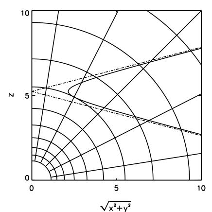
Figure 4: An example of a long characteristic in an axially symmetric space. Only the upper quadrant is shown. The vertical axis is the symmetry axis and the horizontal axis the equator. The bot-dashed lines represent the asymptotes of the hyperbolic characteristic.

For the numerical implementation of the short characteristics scheme, we are interested in those characteristics that pass through a grid point $P=(R_{k},\Theta_{l})$ and are tangent to one of the local discrete ordinates $(\mu_{i},\phi_{j})$. Clearly, once $R_{k},\Theta_{l},\mu_{i},\phi_{j}$ are fixed, such a characteristic is unique and the values of its parameters are

$$b^{2} =R_{k}^{2}(1-\mu^{2}_{i})$$ (33)

$$\cos\Theta_{\infty} =\mu_{i}\cos\Theta_{l}+\sqrt{1-\mu_{i}^{2}}\,\sin\Theta_{l}\sin\phi_{j}$$ (34)

$$z_{0} =R_{k}\big{[}(1-\mu^{2}_{i})\,\cos\Theta_{l}-$$

$$\quad\quad\mu_{i}\sqrt{1-\mu^{2}_{i}}\sin\Theta_{l}\sin\phi_{j}\big{]}\,.$$ (35)

The short characteristic passing through $(R_{k},\Theta_{l}\,;\,\mu_{i},\phi_{j})$ is defined as the section of this curve that starts at the closest intersection with the grid lines upstream of $P$ (point $U$), passes through $P$ and ends at the closest intersection with the grid lines downstream of $P$ (point $D$). The location of the points $U$ and $D$ is specified by the corresponding values of parameter $s$ along the ray, $s_{U}$ and $s_{D}$, which are found solving equations (29)–(30) with $R=R_{K}$ and $\Theta=\Theta_{L}$, where $K=k-1,k,k+1$ and $L=l-1,l,l+1$. Both $R=R_{k}$ and $\Theta=\Theta_{l}$ need to be included because the characteristic may intersect the same $\Theta$ or $R$ grid line twice. In principle, each equation has two solutions for a given value of $K$ and $L$, giving 12 possible roots

$$s_{1\ldots 6} = \pm\sqrt{R_{K}^{2}-b^{2}}$$ (36)

$$s_{7\ldots 12} = \frac{1}{\cos^{2}\Theta_{\infty}-\cos^{2}\Theta_{L}}\bigg{\{}-z_{0}\cos\Theta_{\infty}\pm$$ (37)

$$\cos\Theta_{L}\sqrt{b^{2}(\cos^{2}\Theta_{\infty}-\cos^{2}\Theta_{L})+z_{0}^{2}}\bigg{\}}\,.$$

However, two of these solutions always give $s=s_{P}$, i.e. $P=(R_{k},\Theta_{l})$ itself, and are of no interest. Of the remaining 10 roots, some are complex and must be rejected. Between the real solutions, the one representing point $D$ ($U$) is selected asking that $s>s_{P}$ ($s<s_{P}$) and that $|s-s_{P}|$ is minimum. For convenience, in the following we will denote with $\tilde{R}_{1}$, $\tilde{\Theta}_{1}$, $\tilde{\mu}_{1}$ and $\tilde{\phi}_{1}$ the values of the independent variables along the ray at point $U$.

Although, as we have just shown, short characteristics can be easily defined in spherical coordinates, two major problems have to be solved before they can be of any use in building a transfer algorithm. The first point concerns the fact that, as it was mentioned earlier, $\mu$ and $\phi$ change along the ray. This means that in addition to spatial interpolation (see Eq. 17), we are forced to interpolate in $\mu$ and $\phi$ as well in order to evaluate $I_{\nu}(U,{\boldsymbol{\omega}}{})$. This is because the intensities at points $A$, $B$ and $C$ are known only for a discrete set of directions which are different, in general, from ($\tilde{\mu}_{1}\,,\tilde{\phi}_{1})$.

The second, more fundamental difficulty arises because in spherical coordinates the concept of upstream and downstream boundaries is different from the Cartesian case. Radial infinity is both the upstream and the downstream boundary, while in $\Theta$ there is no obvious upstream or downstream boundary. If the grid is swept from $\Theta=0$ to $\Theta=\pi$ or vice versa, one will encounter situations in which the intensity at one of the points $A$, $B$, $C$ is not known before the evaluation the transfer integral along the short characteristic (Eq. 16) is performed. An example of such a situation is shown in Fig. 5. Interpolation makes use of the points $A$, $B$ and $C$, but since $A$ coincides with $P$, the intensity at the point $A\equiv P$, has not been computed yet.

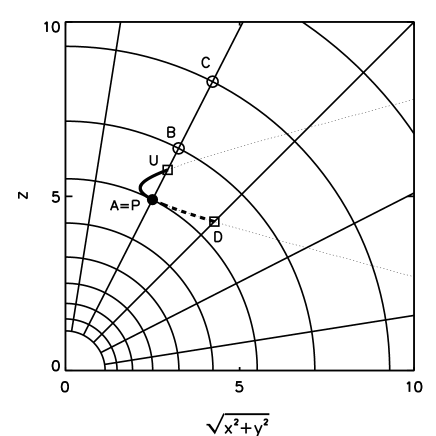
Figure 5: An example of a Short Characteristic (SC) in spherical coordinates (the heavy line connecting $U$ to $D$ through $P$). As in Fig. 2 the downstream part of the SC (which is only needed to guarantee second order accuracy in the formal integral between $U$ and $P$) is dashed. The dotted line shows the complete ray to which the SC belongs.

4.1 Extended Short Characteristics

The problem of unknown intensities can be solved by modifying the definition of short characteristics to be the part of the ray that connects $P$, not with just the nearest gridline intersection, but with the nearest $R=R_{k}$ gridline intersection, i.e. the nearest radial shell. Such an “extended short characteristic” (ESC) is illustrated in Fig. 6.

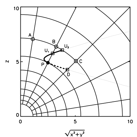
Figure 6: An example of an Extended Short Characteristic (ESC) in spherical coordinates (the heavy line connecting $U_{2}$ to $D$ through $P$). It is the extended version of the SC shown in Fig. 5. The ESC does not have the same problems as the SC because for the ESC none of the points $A$, $B$ or $C$ coincides with point $P$.

The starting point $U$ of such an ESC will be located either at $R=R_{k-1}$, $R=R_{k+1}$ or back at $R=R_{k}$. This means that in between $U$ and $P$ the ESC may intersect one or more $\Theta$ grid lines. The point $D$ on the downstream side remains the same as for standard SCs.

By using ESC instead of SC the “problem of unknown upstream intensities” can be eliminated. In fact, if a proper sweeping scheme is chosen (see Subsection 4.2), the problem of unknown intensities only occurs in those situations when a short characteristic curves back onto the same $\Theta$-gridline from which it originates, as is illustrated in Fig. 5. By extending only those short characteristics, and leaving the rest truly short, one can also avoid unknown intensities in the sweeping scheme. Just for notation we call this scheme the Minimally Extended Short Characteristics scheme (MESC). MESC is almost as accurate as ESC, but ESC is more closely similar to its one-dimensional spherical analogues, and is slightly less numerically diffusive.

In the following we denote with $D$ (or $U_{-1}$) the single downstream intersection with a grid line, and with $U_{i}\ (i=1,\ldots,m)$ the multiple intersections upstream of $P$. The point $U_{m}$ is therefore the true upstream starting point of the ESC, where the intensity must be found by interpolation. In Fig. 6 this is the point $U_{2}$ and the ESC consists of two segments in this case.

4.2 The sweeping scheme

Using the (minimally) extended short characteristics defined above, we can systematically sweep the grid without encountering unknown intensities. We start at the outer boundary $R_{\infty}$ and integrate inwards only those ESCs for which $\mu_{i}\leq 0$. The sweeping order in $\Theta$ is from $\Theta=0$ to $\Theta=\pi$ and then back.

The intensity at each $P=(R_{k},\Theta_{l})$ is found for all $\mu_{i}\leq 0$ and $\phi_{j}$ by tracing the ESCs back to their upstream starting point $U_{m}$. At point $U_{m}$ the values of $R$, $\Theta$, $\mu$ and $\phi$ are different from those at $P$, and will be denoted with $\tilde{R}_{m}$, $\tilde{\Theta}_{m}$, $\tilde{\mu}_{m}$ and $\tilde{\phi}_{m}$. The find the intensity at $(\tilde{R}_{m},\tilde{\Theta}_{m},\tilde{\mu}_{m},\tilde{\phi}_{m}))$ by interpolation. We then integrate the formal transfer equation along each segment of the ESC connecting $U_{m}$ to $P$, according to Eq.(18). This gives

$$\begin{split}I_{\nu}(P)=&\exp(-\tau_{m})I_{\nu}(U_{m})+\sum_{i=1,m}\exp(-\tau_{i-1})\times\\ &\big{(}u_{\nu,i}S_{\nu,i}+p_{\nu,i-1}S_{\nu,i-1}+d_{\nu,i-2}S_{\nu,i-2}\big{)}\end{split}$$ (38)

where $\tau_{i}$ is the depth from $P$ to $U_{i}$ and the index $i$ denotes the quantity evaluated at $U_{i}$ (e.g. $S_{i}\equiv S(U_{i})$; $i=0$ refers to $P$ and $i=-1$ to $D$). The $u$’s, $p$’s and $d$’s are defined as in equations (19), (20) and (21), but with $\tau$ replaced by $(\tau_{i}-\tau_{i-1})$ and $\bar{\tau}$ by $(\tau_{i-1}-\tau_{i-2})$.

The integration is then repeated moving towards smaller radii, until the inner boundary at $R=R_{1}$ is reached. Here we can include the contribution of a central source or any other boundary condition.

Then we start integrating back towards larger radii, until we reach the outer edge. By now the radiation field on the grid $I_{\nu}(R_{k},\Theta_{l}\,;\,\mu_{i},\phi_{j})$ is known.

4.3 Tangent-ray discretization of photon direction

Equations (31) and (32) show that $\mu$ and $\phi$ change along the ESC. If we follow the ESC upstream towards a point $U_{m}$ (see Fig. 6), then the values of these two angles at $U_{m}$ are generally not exactly at the discrete values $\{\mu_{i}\}$ and $\{\phi_{j}\}$ of the sample of directions. This means that we must interpolate not only in space (between $A$, $B$ and $C$), but also in direction $\mu$, $\phi$. Although, this is not, in principle, a fundamental problem, the use of interpolations should be reduced to a minimum to avoid unnecessary numerical diffusion.

Fortunately one can eliminate the interpolation in $\mu$ by means of a suitable choice of the $\mu$–grid so that all ESCs always start and end at one of the $\{\mu_{i}\}$ points. We let the $\mu$–discretization depend on $R_{k}$,

$$\{\mu_{k,j}\,;\,j=-m_{k},\cdots,m_{k}\}\,,$$ (39)

and choose the $\mu_{k,j}$ in such a way that for each $j=-m_{k},\cdots,m_{k}$ there is a $j^{\prime}=-m_{k-1},\cdots,m_{k-1}$ such that

$$(1-\mu_{k,j}^{2})R^{2}_{k}=(1-\mu_{k-1,j^{\prime}}^{2})R^{2}_{k-1}\,.$$ (40)

This choice is based on the fact that the values of $\mu$ and $R$ along an ESC depend only on each other and on $b{}$, as can be seen by combining equations (29) and (31):

$$(1-\mu^{2})R^{2}=b{}^{2}\,.$$ (41)

By choosing the $\mu_{k,j}$ according to Eq.(40), a ray which originates at $R_{k}$ with, say, $\mu=\mu_{k,j}$ and arbitrary $\phi$, reaches any other radius along the path with a value of $\mu$ which coincides with one of the points of the local $\mu$ grid there, thus eliminating the need for interpolation.

A $\mu$-grid that is consistent with Eq.(40) is:

$$\mu_{k,\pm i}=\pm\sqrt{1-\frac{R^{2}_{k-i}}{R^{2}_{k}}}\,,$$ (42)

in agreement with the angular spacing induced in spherical symmetry by the “tangent ray method” (see e.g. Mihalas Mihalas et al. (1975); Zane et al. Zane et al. (1996)). Actually, it can be easily shown that in 1-D spherical symmetry the ESC method, with $\mu_{k,j}$ given by Eq.(42), is fully equivalent to the tangent ray method. This is an important feature of the algorithm since it then exactly recognizes spherical symmetry. And, even in the absence of spherical symmetry, it transports radiation outward without any numerical diffusion in $R$ or $\mu$.

However, the $\mu$ spacing implied by Eq.(42) has the tendency to give a poor sampling around $\mu=0$. This problem can be easily solved by introducing some (typically one or two) extra points around $\mu\simeq 0$ to enhance the angular resolution there. Obviously this violates the original prescription and therefore requires the use of interpolation for these extra $\mu$–points, producing a small amount of angular diffusion for $\mu\sim 0$. Generally this diffusion is small.

Unfortunately the interpolation in $\phi$ can never be avoided. The $\phi$ angle depends in a complicated way on $s$ (see Eq. 32) and it can change rapidly even within one element of a ESC. Both first and higher order interpolation in $\phi$ have been tested in our numerical code. We have found that in most cases the $\phi$ diffusion is not very large and, in general, influences the solution less than the spatial ($\Theta$) diffusion.

4.4 Special treatment of radiation near $\mu\simeq 1$

The tangent-ray discretization of $\mu$ allows the algorithm to accurately conserve radial flux. However, such a choice of $\mu$–angles requires a large number of $\mu$ points at larger radii, typically $m_{k}\gtrsim k$. One cannot make do with a smaller number of $\mu$ points without facing the risk of loosing flux. This is illustrated in the following argument. If radiation is emitted at a radius $R$, an observer at $R_{k}\gg R$ can see the radiation from the emitting region even if its eyes cannot resolve the source. This is because the observer’s eyes measure the flux and not the intensity. The ESC algorithm, on the other hand, deals with intensity, and intensity is converted into flux by performing an integral over $d\mu\,d\phi$. For this integral to be reasonably accurate, the emitting region must be resolved in $\phi$ and $\mu$, leading to the requirement $m_{k}\gtrsim k$.

Unfortunately this means that the computational cost scales as $N_{R}^{2}$ if one wishes to extend the span of the radial domain. Since the ability to deal with many orders of magnitude in radius is crucial to solving transfer problems in circumstellar envelopes, this scaling is undesirable.

An easy way to solve this scaling problem is related to the simple observation that all photons with $\mu\simeq 1$ follow roughly a radially outgoing trajectory and they tend to travel more radially (i.e. with $\mu$ closer to unity), the further they propagate outwards. In the “radial streaming” limit ($1-\mu\ll 1$), Eq.(40) becomes approximately

$$\frac{1-\mu_{k,j}}{1-\mu_{k-l,j-l}}=\frac{\Omega_{k,j}}{\Omega_{k-l,j-l}}\simeq\frac{R^{2}_{k-l}}{R^{2}_{k}}$$ (43)

where $\Omega_{k,j}$ is the solid angle (bounded by $\mu_{k,j}$) at $R_{k}$. Eq.(43) is just a restatement of the $1/R^{2}$ law which is exactly obeyed by a point source and by any radiation in the radial streaming limit.

This property of radially outward radiation makes it possible to bundle all $\mu$–points with sufficiently large $\mu$ into a single collective flux-like bin. The intensity of that bin will be treated as the average intensity within that collective bin. The idea is to divide the $\mu$–range $[-1,1]$ into three parts

$$[1,-\mu_{rs}] \mu \simeq-1$$ inward intensity bin:

$$[-\mu_{rs},\mu_{rs}] \mu =\mu_{k,j}$$ intensity samples:

$$[\mu_{rs},1] \mu \simeq 1\,.$$ outward averaged bin:

This way the number of $\mu$–gridpoints $m_{k}$ at each radius can be limited, depending on how close $\mu_{rs}$ is to unity. We choose a global value for $\mu_{rs}$, and do not allow this to differ from one radius to another.

Because the radial outward bin represents an integrated intensity, i.e. an average of the true intensity over a solid angle $\Omega_{rs}=2\pi(1-\mu_{rs})$, it requires a special treatment. Let us denote the average intensity in this bin as $I^{+}_{\nu}(R_{k},\Theta_{l})$. The integration formula, Eq.(38), for $I^{+}_{\nu}(R_{k},\Theta_{l})$ becomes

$$\begin{split}I^{+}_{\nu}(&R_{k},\Theta_{l})=\exp(-\tau)\bigg{[}\frac{R^{2}_{k-1}}{R^{2}_{k}}I^{+}_{\nu}(R_{k-1},\Theta_{l})+\\ &\left(1-\frac{R^{2}_{k-1}}{R^{2}_{k}}\right)\frac{1}{2\pi}\int_{0}^{2\pi}I_{\nu}(R_{k-1},\Theta\,;\,\mu_{m_{k}-1},\phi)\,d\phi\bigg{]}\\ &+u_{\nu}S_{\nu}(R_{k-1},\Theta_{l})+p_{\nu}S_{\nu}(R_{k},\Theta_{l})\\ &+d_{\nu}S_{\nu}(R_{k+1},\Theta_{l})\,.\end{split}$$ (44)

This formula simulates the correct $1/R^{2}$ behavior of the flux for optically thin media provided $\mu_{rs}$ is sufficiently close to unity. It reduces to the standard expression when the medium is optically thick. An estimate of the error introduced by the assumption of radial streaming can be made by comparing equations (40) and (43), and is of order $(1-\mu_{rs})/2$. The radiation contained in the $\mu=1$ bin will not accumulate any numerical interpolation errors because it moves strictly along the radial grid lines.

The inward collective bin will always behave as a real intensity, so that the $1/R^{2}$ behavior does not need to be simulated.

4.5 Spectra and images

Once the iterative part of the transfer has been completed and the source function is known, the next step is to produce images and spectra. An image is produced by formal integration of the source function along long characteristics through the medium (ray tracing). Each ray represents one pixel of the image. One can produce spectra by making images at a range of frequencies, and integrating these images over the “detector” aperture.

Here, as in the Lambda iteration, we face resolution problems if the source under consideration spans a large range in $\log(R)$. The central parts of the image are often much brighter than the rest, but cover a much smaller fraction of the image. The spectrum may therefore contain significant contributions of flux from both the central parts and the outer regions of the image. Unless the image resolve all spatial scales of the object, the spectra produced in such a way are unreliable.

If a rectangular arrangement of pixels is used, one must make sure to use a variable spacing in both $x$ and $y$, in such a way that the small scales around the star are sufficiently resolved. If one is mainly interested in the images themselves, this seems the most reliable and straightforward way to go.

For the production of spectra we propose a different approach. Rather than arranging the pixels over a rectangle, we arrange them in concentric rings. The impact parameters of the circles are related to the radial grid points of the transfer calculation. For a reliable evaluation of the spectra it is generally enough to have one circle for each $R_{i}$, plus some more, about 5, to resolve the central region. The number of circles $N_{b}$ in each image is therefore roughly the same as the number of radial grid points: $N_{b}=N_{R}+5$. The number of pixels in each circle $N_{\varphi}$ is slightly less straightforward to choose, but for reliable spectra it is generally sufficient to take $N_{\varphi}=2N_{\Theta}$, where $N_{\Theta}$ is the number of $\Theta$ grid points, counted from pole to pole. Using this method, the images automatically resolve all relevant scales, while using only a fairly limited number of pixels.

5 Testing the ESC Lambda Operator

The Extended Short Characteristic implementation of the Lambda Operator is not exact, as opposed to the one based on Long Characteristics. The interpolations used in the ESC algorithm introduce numerical diffusion, even in the optically thin regime, and this constitutes a potential threat to the reliability of the method. In order to test the accuracy of the ESC Lambda Operator we have performed a series of runs for a number of simple setups, comparing the results of the ESC calculation with those obtained by means of an exact LC Lambda Operator. Here we present the analysis for three such tests.

5.1 Optically thick annulus

The first test problem concerns the determination of the radiation field produced by an optically thick, isothermal, sharply–edged annuls, bounded by $R_{0}<R<R_{M}$ and $\Theta_{M}<\Theta<\pi-\Theta_{M}$. In the actual calculation we have taken $R_{0}=2.86$, $R_{M}=4.83$, $\Theta_{M}=1.26$ and the absorbtion $\alpha_{a}$ is given by

$$\alpha_{a}(R,\Theta)=\left\{\begin{matrix}10^{3}&\hbox{inside the annulus}\\ 0&\hbox{elsewhere}\,.\\ \end{matrix}\right.$$ (45)

For the sake of simplicity all variables are dimensionless and the temperature has been taken such that $B_{\nu}(T)=1$. We use a spatial grid with $20$ radial points, logarithmically spaced such that

$$\frac{R_{i+1}-R_{i}}{R_{i}}=1.1402\,,$$

and the angular grid in $\Theta$ consists of 20 equally spaced points from pole to pole. Fig. 7

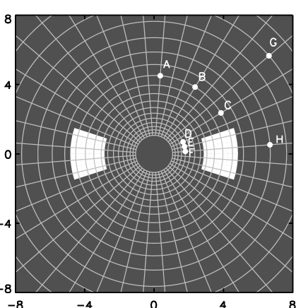
Figure 7: The set–up for the test runs. The annulus is shown together with the spatial mesh. Here all four quadrants are shown, although only the first quadrant needs to be computed as a result of mirror symmetry in the equatorial plane and cyclindrical symmetry around the polar axis. Nine representative grid points, labeled $A-H$, are marked (see Fig. 8).

shows the configuration for the test problem. Mirror symmetry in the equator reduces the number of actual points to 10 in the range $0<\Theta<\pi/2$. The mesh in photon momentum space consists of 32 equally spaced points in $\phi$, covering the range 0–$2\pi$, and 41 points in $\mu$, 38 chosen according to Eq.(40), plus $\mu=0$ and $\mu=\pm 0.24$ to ensure sufficient resolution at small $\mu$. Because of the symmetry, the transfer needs to be solved only for the 16 points in the ranges $0<\phi\leq\pi/2$ and $3\pi/2<\phi\leq 2\pi$.

The radiation field emitted by such a source can be semi–analytically determined. As seen by an observer at some point $P$, it is simply the projection of the object on the sky of the observer. Since the object is sharply–edged and highly optically thick ($\tau\gg 100$), its projection will be sharply–edged as well. The intensity is simply given by

$$I_{\nu}(P\,;\,\mu,\phi)=\left\{\begin{matrix}0&\hbox{for rays missing the object}\\ B_{\nu}(T)&\hbox{for rays hitting the object}\\ \end{matrix}\right.\;,$$ (46)

so it is easy to compute the projections on the sky of the observer at various positions in space by using some independent ray–tracing algorithm or a semi–analytical computation of the image. This image can then be compared to that produced by the ESC and the LC transfer algorithms to evaluate the accuracy of the ESC Lambda Operator.

Let $I_{ESC}(\mu,\phi)$ and $I_{LC}(\mu,\phi)$ be the intensities, at the observer location, computed using the ESC and the LC algorithms, for the same discretization in $\mu$ and $\phi$. Let, moreover, $I(\mu,\phi)$ be the true intensity, which may be found by tracing individual rays with very high resolution in $\mu$ and $\phi$. We define the standard error of the ESC algorithm as

$$\sigma^{2}_{ESC}=\frac{\int(I_{ESC}-I)^{2}d\mu d\phi}{\int I^{2}d\mu d\phi}$$ (47)

and the error in the mean intensity $J$ as

$$\epsilon_{ESC}=\frac{\int(I_{ESC}-I)d\mu d\phi}{\int Id\mu d\phi}\equiv\frac{J_{ESC}-J}{J}\,.$$ (48)

Similar definitions apply to the LC errors.

Radiative transfer for this setup has been performed using the ESC method. The results are shown in Fig. 8 for the 9 gridpoints labeled $A-I$ in Fig. 7.

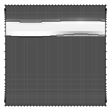
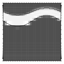
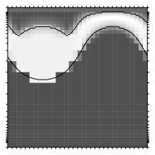
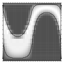
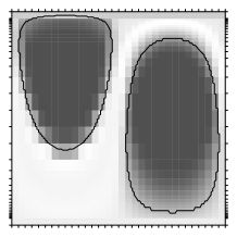
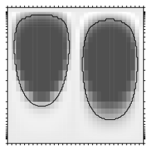
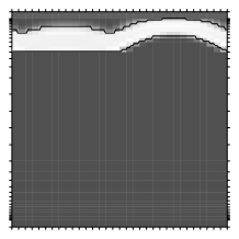
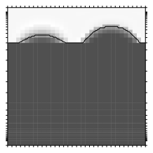
Figure 8: The radiation field $I(\mu,\phi)$ for the test problem of the optically thick annulus at various positions in space (from top left to bottom right at the points $A-H$ of Fig. 7). In each panel $\phi$, from 0 to $2\pi$, is on the $x$–axis and $\mu$, from -1 to 1, on the $y$–axis. Tickmarks on both axes are representative of the actual values of $\mu$ and $\phi$ used in the calculation. The image shows the intensity resulting from the ESC transfer algorithm (the grey scale is such that white corresponds to maximum and black to zero). The thin solid curves mark the true contour of the object, computed by ray–tracing with high angular resolution. The slightly diffusive nature of the results is a consequence of the interpolations inherent to the ESC method. Numerical diffusion remains quite low in almost all cases, with the possible exception of point $E$.

The contours of the real images are overplotted. The same calculation has been repeated using the LC method. The errors of both the ESC and the LC calculations are listed in Table 1. These figures show that the errors of the ESC method are not very much greater than those of the LC method (which result from the discretization alone) and strenghten the reliability of the ESC algorithm.

Point $\epsilon_{ESC}$ $\sigma^{2}_{ESC}$ $\epsilon_{LC}$ $\sigma^{2}_{LC}$ A $0.060$ $0.090$ $0.085$ $0.116$ B $0.034$ $0.112$ $-0.016$ $0.134$ C $0.059$ $0.112$ $0.001$ $0.105$ D $-0.020$ $0.091$ $0.002$ $0.094$ E $0.107$ $0.096$ $-0.032$ $0.084$ F $0.109$ $0.103$ $0.028$ $0.089$ G $0.029$ $0.051$ $-0.019$ $0.068$ H $-0.012$ $0.056$ $-0.046$ $0.104$

Table 1: The errors of ESC and the LC algorithms for the optically thick test.

5.2 Optically thin annulus

Contrary to the optically thick case of the previous subsection, the radiation field from an optically thin annulus cannot be determined by a simple analytic formula such as Eq.(46). At large radii, however, the mean intensity should follow the $1/R^{2}$ law and be independent of $\Theta$. We can verify if the solution produced by the ESC algorithm indeed has this expected behavior. All details are the same as in the previous test, with the only difference that now the (constant) absorption is taken $10^{-6}$.

We focus on the behavior at large radii. In radial streaming $H(R_{i},\Theta_{j})\simeq J(R_{i},\Theta_{j})$ which, for an optically thin source, is simply proportional to the volume integral of the emissivity $j(R,\Theta)$ and is independent of $\Theta$

$$J(R)=\frac{1}{4\pi R^{2}}\int j(R^{\prime},\Theta^{\prime})(R^{\prime})^{2}dR^{\prime}\sin\Theta^{\prime}d\Theta^{\prime}\,.$$ (49)

Although close to the source the mean intensity is still very dependent on $\Theta$, at $R\gg R_{M}$ the code should be able to recover the correct behaviour $J\propto R^{-2}$ at large radii. The mean intensity $J(R_{i},\Theta_{J})$ resulting from the ESC transfer calculation is shown in Fig. 9, where it is multiplied with $R^{2}$. It can be clearly seen that the while $J$ depends on $\Theta$ for small radii, it becomes almost independent on $\Theta$ as the radius increases and that the inverse square law is very well reproduced. The dependence of $J$ on $\Theta$ at the largest radius is shown in Fig. 10. Typical errors are $\lesssim 5\%$, which lies within the error expected from the coarseness of the grid.

Figure 9: A surface plot of the mean intensty $J(R,\Theta)$ as produced by the ESC algorithm for the optically thin annulus. In order to show the behavior at large radii, the mean intensity is multiplied by $R^{2}$ and normalized for convenience.

Figure 10: The computed (solid line) and the exact (dashed line) mean intensity for the optically thin annulus, at the largest radius as a function of $\Theta$; errors are $\lesssim 5\%$.

5.3 Spherically symmetric test problem

Although the above tests show that the ESC algorithm performs well on its own, they are not enough to prove that it will produce accurate and reliable results when applied to, for instance, a non–LTE line transfer computation. Unfortunately it is not easy to test this, because to our knowledge there exists no useful benchmark test case yet for 2–D axisymmetric radiative transfer in circumstellar clouds.

The least we can do is to test our 2–D algorithm on a 1–D spherically symmetric test case, and check the output against that produced by an independent 1–D transfer calculation. This way we can at least test two of the special features of the ESC algorithm: the additional $\mu$-points close to $\mu\simeq 0$, and the special treatment of the intensity near $\mu\simeq 1$. These are features that are not particularly related to 2-D, and can therefore also be tested in 1-D just as well.

Our test cloud is a spherically symmetric power law model with hydrogen density specified by

$$N_{{\hbox{H}_{2}}}(R)=N_{{\hbox{H}_{2}}}^{0}\;\left(\frac{R_{0}}{R}\right)^{2}\quad\hbox{cm}^{-3}\,,$$ (50)

where $R$ is the radius in cm, and $N_{{\hbox{H}_{2}}}^{0}=2.0\times 10^{7}\,\hbox{cm}^{-3}$ is the number density at $R=R_{0}\equiv 1.0\times 10^{15}\,\hbox{cm}$. We take a constant kinetic temperature $T_{\hbox{{\scriptsize kin}}}(R)=20\,\hbox{K}$. The abundance of our molecule is also a constant, $X_{\hbox{{\scriptsize mol}}}(R)\equiv N_{\hbox{{\scriptsize mol}}}(R)/N_{{\hbox{H}_{2}}}(R)=1.0\times 10^{-6}$. The systematic velocity is taken zero. The models are computed in spherical coordinates, in the domain $R_{\hbox{{\scriptsize in}}}\leq R\leq R_{\hbox{{\scriptsize out}}}$. We take $R_{\hbox{{\scriptsize in}}}=1.0\times 10^{15}\,\hbox{cm}$ and $R_{\hbox{{\scriptsize out}}}=7.8\times 10^{18}\,\hbox{cm}$. At the inner boundary we put a reflective boundary condition. The incoming radiation at the outer boundary is the $T=2.728\;\hbox{K}$ microwave background radiation.

We choose a fictive 2-level molecule which is specified by

$$E_{2}-E_{1} =6.0\;\hbox{cm}^{-1}=8.63244\;\hbox{K}$$ (51)

$$g_{2}/g_{1} =3.0$$ (52)

$$A_{21} =1.0\times 10^{-4}\;\hbox{s}^{-1}$$ (53)

$$K_{21} =2.0\times 10^{-10}\;\hbox{cm}^{3}\,\hbox{s}^{-1}$$ (54)

from which the downward collision rate follows: $C_{21}=N_{{\hbox{H}_{2}}}K_{21}\;\hbox{s}^{-1}$. The total (thermal+turbulent) line width $a_{\hbox{\scriptsize tot}}$ is $a_{\hbox{\scriptsize tot}}=0.150\;\hbox{km}\,\hbox{s}^{-1}$ (see Eq. 6).

The test problem presented here has high optical depth and a very sub-critical density. It is therefore well suited to test whether non-LTE effects are properly computed.

The line transfer is computed in a passband of 40 frequency points equally spaced between $-0.40\;\hbox{km}\,\hbox{s}^{-1}$ and $+0.40\;\hbox{km}\,\hbox{s}^{-1}$. The $\mu$ angle is discretized using $43$ points, arranged according to the tangent-ray prescription of Eq.(42) with $3$ additional $\mu$-points around $\mu=0$ on each side. Our convergence criterion is simply:

$$\max(\delta n_{i}/n_{i})<1\times 10^{-4}$$ (55)

at all radii. For the radius we use an equally spaced logarithmic grid with $(R_{i+1}-R_{i})/R_{i}\equiv\Delta R/R=0.1720$. We perform 4 runs: Lambda Iteration and Accelerated Lambda Iteration with and witout Ng acceleration.

The results for the upper level population is plotted in Fig. 11 and compared to the results obtained independently with SIMLINE written by V. Ossenkopf (Ossenkopf (1999)). The convergence plots for four different methods are shown in Fig. 12.

Figure 11: The fractional population of the upper level of the 1-D test problem. The symbols are the solution produced by RADICAL, which is our code based on the ESC algorithm. ALI+Ng were used. The solid line is the solution found by the program SIMLINE, which is an independent 1-D line transfer program written by V. Ossenkopf (Ossenkopf (1999)). The difference between the two solutions (normalized to the SIMLINE solution) is shown in the lower panels.

Figure 12: Convergence plot for the 1-D test problem. The largest error is plotted against the iteration number for four different methods. We define the error as the maximum relative difference between the “real” solution and the level populations at iteration $N_{\hbox{\scriptsize iter}}$. The “real” solution was obtained with ALI+Ng and converged down to $\max(\delta n_{i}/n_{i})<10^{-6}$, which is a 100 times stricter convergence criterion than the last iteration step plotted for ALI+Ng in this figure.

More test problems, and a more extensive discussion of them was presented by Dullemond (Dullemond (1999)).

6 A simple model for the Egg Nebula

Now that the algorithm has been tested, we demonstrate here how it can be used in practice. Our first example is a simple model of the optical appearance of the Cygnus Egg Nebula (CRL 2688). This object has been extensively studied ever since its discovery by Ney et al. (Ney et al. (1975)). It is a bipolar reflection nebula surrounding an F5 supergiant of $T_{\hbox{{\scriptsize eff}}}=6500\hbox{K}$ (Crampton Crampton et al. (1975)). At optical wavelength it appears as a diffuse bi–lobed nebula with two sharply edged “searchlight beams” emerging from each of the poles (Sahai et al. Sahai et al. (1998)). The lobes are separated by a dark equatorial lane which completely obscures the central star.

The optical emission from this nebula can be understood as reflected starlight escaping from the nebula through polar cavities (Latter et al.Latter et al. (1993), Morris Morris (1981)). It is clear that the “searchlight beams” are due to single scattering of direct starlight by dust grains. The lobes are, however, more likely to be the result of multiple–scattering.

We will model this multiple–scattering process in 2–D with the MESC algorithm, in an attempt to reproduce the complex optical appearance of the nebula. Our setup consists of an almost spherical wind with a cavity at both poles. The density in the cavities is small, but it is still high enough to reflect sufficient amounts of starlight. To reproduce the twin–beams at both poles, we place a small blob of matter at the polar axis in the cavity, causing a shadow. A star is placed at the center of the coordinate system to illuminate the nebula from within.

We model only a single frequency in the optical, at 600 nm. For this reason we refrain from taking actual realistic dust opacities, and specify total optical depth and scattering albedo instead. The dust density is shown as contour plots in Fig. 13. The total optical depth at the equator is about 60. The ratio of absorption over scattering is $0.3$. The dust scattering is assumed to be isotropic, which suffices for the present simplified example. We do not specify the dust temperature for this setup since thermal emission at 600 nm is negligible.

The simulation was performed by RADICAL, using the MESC algorithm, and applying Accelerated Lambda Iteration and Ng acceleration. The image subsequently produced by formal integration is shown in Fig. 14. The model reproduces the searchlight beams and the diffuse glow. It also naturally reproduces the intensity difference between the north and south lobe. This is a result of the slight inclination at which the object is seen. For light emerging from the south lobe, the path length through the outer regions of the nebula is larger than for the north lobe.

Figure 13: The density contours for the dust envelope around the central star of the Egg Nebula. Contours are logarithmically spaced, separated by factors of $\sqrt{10}$. The distance scale on the x- and y-axis is in centimeters. At the polar axis one can see a small blob of matter. This blob is responsible for the shadow.

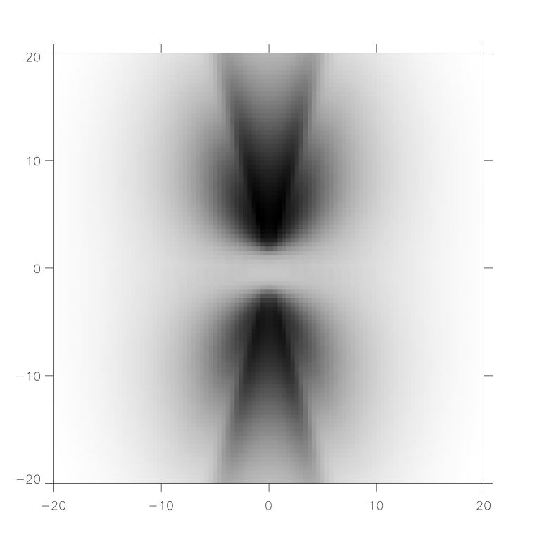
Figure 14: The synthetic image of the Egg Nebula, produced by RADICAL. The color coding is reverse logarithmic grey scale. The color table was slightly modified to enhance contrast in the lobes, but the modifications remain within 15%.

Although the model resemblances the HST image of Sahai et al., it should be noted that the density structure that we have used may not be consistent with observations at other wavelengths. For example, HCN observations by Bieging & Nguyen-Q-Rieu (Bieging and Q.-Rieu (1996)) seem to rule out the presence of a cavity in the wind. Also the rather high albedo may be difficult to reconcile with the fact CRL 2688 is carbon–rich.

7 A model of line transfer in a collapsing protostellar cloud

In this section it will be demonstrated how the 2-D transfer algorithm can be used in the observational study of low-mass star formation in dense molecular cloud cores.

Low mass star formation takes place in dense molecular cloud cores. According to the spherically symmetric model of Shu (Shu (1977)), such a core develops a cusp with density close to a $1/R^{2}$ powerlaw. Once a gravitational instability is trigged, the centeral part of the cloud collapses, and forms a star. An expansion wave propagates into the cloud towards larger radii, allowing more and more matter to fall supersonically down the potential well, and add to the protostar’s mass.

Both observational evidence and theoretical arguments, however, indicate that purely spherical collapse is rare. Any slight amount of angular momentum in the primordial cloud will cause deviations from sphericity as centrifugal forces tend to dominate over radial infall deep down the potential well. And even before the collapse stage these primordial clouds often appear to be non-spherical (Myers et al. Myers et al. (1991)). Theoretical models of non-spherical protostellar collapse include, among others, Ulrich (Ulrich (1976)), Cassen & Moosman (Cassen and Moosman (1981)), Terebey et al. (Terebey et al. (1984), Galli & Shu Galli and Shu (1993).

The models of Cassen & Moosman and Ulrich (hereafter CMU) focus on the inner free-falling part of the collapsing cloud, and assume that the material originates from an originally spherical cloud with some angular momentum. Their model is almost spherical at large radii, but flattens off closer towards the center, and forms a disk near the centrifugal radius. This model was later extended by Hartmann et al. (Hartmann et al. (1996), hereafter HCB) to include flattening of the parent cloud. These models show that the inner free-fall part of an initially flattened cloud naturally tends to form a bipolar cavity, which is often observed in YSO. These models are distinctly non-spherical at all radii, despite the fact that centrifugal forces only dominate at small radii. It is therefore evident that fitting such models to molecular line observations requires 2-D axi-symmetric radiative transfer computations.

In this section we perform such a calculation, using the algorithms of this paper. We solve the non-LTE level populations for the first 7 rotational levels of HCO⁺, and compute the predicted single–dish spectra.

7.1 Description of the model

In our HCB models we assume that the radius of the expansion wave ${R_{\hbox{\scriptsize acc}}}$ is outside our domain, so we shall confine our study to the free-fall inner region of the collapsing sheet-like molecular cloud. We assume that matter in the parent cloud had a small amount of rotation in the plane of the sheet before it collapsed. According to the HCB model, the velocity field of the gas is given by the formulae of Ulrich (Ulrich (1976)):

$$v_{R} =-\left(\frac{GM}{R}\right)^{1/2}\left(1+\frac{\mu}{\mu_{0}}\right)^{1/2}$$ (56)

$$v_{\Theta} =\left(\frac{GM}{R}\right)^{1/2}\left(\frac{\mu_{0}-\mu}{\sqrt{1-\mu^{2}}}\right)\left(1+\frac{\mu}{\mu_{0}}\right)^{1/2}$$ (57)

$$v_{\phi} =\left(\frac{GM}{R}\right)^{1/2}\left(\frac{1-\mu_{0}^{2}}{1-\mu^{2}}\right)^{1/2}\left(1-\frac{\mu}{\mu_{0}}\right)^{1/2}\,,$$ (58)

where $\mu\equiv\cos(\Theta)$ and $\mu_{0}\equiv\cos(\Theta_{0})$. The angle $\Theta_{0}$ is the $\Theta$-coordinate that the gas parcel had when it started its free-fall at large radius. For a given $(R,\Theta)$ the value of $\Theta_{0}$ can be found from

$$\frac{R}{{R_{\hbox{\scriptsize c}}}}\left(1-\frac{\mu}{\mu_{0}}\right)=(1-\mu_{0}^{2})\,,$$ (59)

where ${R_{\hbox{\scriptsize c}}}$ is the centrifugal radius, i.e. the radius at which centrifugal forces equal gravity. This is the outer radius of the disk that is formed as a result of the rotation.

The density of the gas for the HCB model is given by

$$\begin{split}\rho_{HCB}(R,\Theta)=&\frac{\dot{M}}{4\pi(GMR^{3})^{1/2}}\frac{\eta\hbox{sech}^{2}(\eta\mu_{0})}{\tanh(\eta)}\\ &\times\left(1+\frac{\mu}{\mu_{0}}\right)^{-1/2}\left(\frac{\mu}{\mu_{0}}+\frac{2\mu_{0}^{2}{R_{\hbox{\scriptsize c}}}}{R}\right)^{-1}\end{split}$$ (60)

where $\eta$ is a dimensionless flattening parameter, which is roughly equal to the ratio of the accretion radius ${R_{\hbox{\scriptsize acc}}}$ to the sheet thickness $H$. HCB argue that this value must be somewhere in between $\eta=0$ and $\eta=\eta_{\hbox{\scriptsize max}}\simeq 4$. For $\eta=0$ the CMU models are reproduced. Density contours of this free-falling envelope, for different flattening parameters, are shown in Fig. 15.

Figure 15: The density structure of the flattened collapsing cloud model of HCB, for varying flattening parameter $\eta$. Scales are in $AU$. The centrifugal radius is at ${R_{\hbox{\scriptsize c}}}=100\;\hbox{AU}$. The effect of rotation can be seen most clearly in the $\eta=0$ case, which is spherical at large radius, but flattens off near $R={R_{\hbox{\scriptsize c}}}$.

The centrifugal radius of the infalling envelope is at ${R_{\hbox{\scriptsize c}}}=100\;\hbox{AU}$. We place a thin disk with a radius of $R_{\hbox{\scriptsize disk}}={R_{\hbox{\scriptsize c}}}=100\;\hbox{AU}$ at the equator. A zoom-in of the density distribution, down to the scale of the disk, is shown in Fig. 16. We will ignore any emission from the disk, and merely treat it as a light-blocking boundary condition at the equator.

      

Figure 16: A zoom-in of the density structure of the $\eta=3$ case of the HCB model. The figure on the right is a zoom-in to the scale of the centrifugal radius. The bar represents the disk.

7.2 Non-LTE line transfer

We compute the line transfer problem for four HCB models, with flattening parameter $\eta=0,1,2,3$ for models 1,2,3,4 respectively. The adopted valued for the accretion rate and the turbulent line width are $\dot{M}=2.4\times 10^{-6}\,M_{\odot}\hbox{yr}^{-1}$ and $a_{\hbox{\scriptsize turb}}=0.25\,\hbox{km}\hbox{s}^{-1}$.

For these models we compute the non-LTE line transfer problem of the lowest few rotational levels of HCO⁺, including the effects of the moving medium. We assume a cosmic background (CMB) continuum as incident radiation at the outer edge of the computational domain. Dust emission and opacity are neglected in the line transfer, which is justified for the lower-lying HCO⁺ lines because the nebula is optically thin to dust in the millimeter and sub-millimeter, and radiative pumping by dust continuum is not important for HCO⁺. Also, we need not include the dust emissivity in the computation of the emerging spectra, since we shall show only the spectra with the dust- and CMB-continuum removed. The radiative transfer is computed within a range of $R\in[70,10^{4}]\,\hbox{AU}$. As an inner boundary we have a vacuum. The cross sections for H₂-HCO⁺ collisional transitions were taken from Monteiro (Monteiro (1985)) and Green (Green (1975)). We adopt an HCO⁺ abundance of $2\times 10^{-9}$ The gas temperature is taken to be $T=20\hbox{K}$ throughout the cloud.

We perform the non-LTE line transfer for all four models. The resulting non-LTE level populations for model 3 are shown in Fig. 17, and the corresponding excitation temperatures are shown in Fig. 18. One can see that at the equator ($\Theta=\pi/2$) the levels are almost thermalized, except at large radii. This is due to the much larger density at the equator than at the pole. The drop in excitation temperature at large radii is a result of the decoupling of radiation and matter. At large radii the level populations will be strongly influenced by the cosmic background radiation. Another interesting phenomenon occurs at small radii near the pole: the excitation temperature exceeds the gas temperature. This effect was discussed by Leung & Liszt (Leung and Liszt (1976)) for the CO 1-0 transition. It can be understood as resulting from an overpopulation of the $J=1$ level due to the large ratio of radiative rates ($A_{21}/A_{10}\simeq 10$).

Once the level populations have been computed, the line spectra are produced. The spectra are centered on the origin of the object. First the circular images are produces in a range of frequencies. This circular rendering of the images ensures that no details at large or small radii are missed, and thus that no flux is accidently lost. The antenna temperatures are then computed by integrating the images, after they have been multiplied by the beam pattern centered on the origin of the object. We use an “Airy” beam, with a beam size corresponding to a single dish of 15 m diameter. The object is placed at 140 parsec distance. The spectra of the four models, computed for the first four radiative transitions at three different inclinations, are shown in Fig. 19.

From the spectra one can clearly see the effect of flattening of the HCB cloud, in particular for models 3 and 4. At near pole-on inclination (5^∘) hardly any self-absorption is seen in these models, because one looks straight into the “cavity”. At near edge-on inclination (85^∘) the “torus” blocks the central regions from view near line center, which results in the clear self-absorption features seen in the line shapes. A similar manifestation of the non-spherical symmetry of the cloud has been discussed recently by Van der Tak et al. van der Tak et al. (1999). An interesting feature of the line spectra of models 3 and 4 is that the edge-on line profiles are wider than the pole-on profiles. This can be attributed to the fact that the density and the excitation temperature is lower at the pole than at the equator. At pole-on inclination the high density equatorial matter will emit near line-center instead of in the line wings, thus making the line profile narrower.

The asymmetry between the red-shifted and the blue-shifted peaks are typical for protostellar collapse. The rotation is hardly seen in these spectra. This is because the rotational velocity is everywhere much smaller than the free-fall velocity, except at very small radii where the emission barely contributes to the single-dish spectra shown here.

   

   

Figure 17: The level populations for model 3 for the first four rotational levels of HCO⁺ as a function of $\Theta$ and $R$. Note that the centrifugal radius (which is the disk outer edge) is at ${R_{\hbox{\scriptsize c}}}=1.5\times 10^{15}\hbox{cm}$.

   

   

Figure 18: The excitation temperatures of the lowest four rotational transitions of HCO⁺ for model 3, as a function of $\Theta$ and $R$. They were deduced from the level populations shown in Fig. 17, using the formula $T_{\hbox{\scriptsize ex}(ij)}=(h\nu_{ij}/k)/\log(n_{j}g_{i}/n_{i}g_{j})$.

Figure 19: The single-dish HCO⁺ line spectra of the HCB models, shown at three different inclinations: dotted line is 5^∘ (near pole-on), dashed line is 45^∘ and solid line is 85^∘ (near edge-on). A dish diameter of 15 m was taken, and the object is located at 140 pc.

8 Conclusions

Numerical radiative transfer modeling on desktop workstations is extremely cheap. Not doing so in cases where this is possible would mean an enormous waste of valuable information that lies encoded in observed data. However the success of such modeling depends on the algorithms that are available. We have developed a robust and accurate method, called the “extended short characteristics” (ESC) method, by which complicated 2–D axi–symmetric multi–frequency radiative transfer calculations can be performed. By using spherical coordinates, this method can accurately treat circumstellar envelopes and disks from the stellar surface all the way up to parsec scale, without the need of grid refinement. By making a special choice of discrete photon angles and bundling ‘almost–radially–moving’ rays into a single bin, the conservation of radial flux can be guaranteed even over many orders of magnitude in radius, and without excessive computational cost.

The ESC method, and a slight variation called MESC, forms the core of a multi–purpose 2-D radiative transfer code called RADICAL. We have tested the ESC/MESC algorithm on a simple test problem which we described in this paper. We have also verified that the 2-D algorithm, when applied to a 1-D spherically symmetric problem, indeed reproduces what an independent 1-D algorithm would produce for the same problem. The errors remained within a few percent, the exact value of which depends on the grid resolution.

The ESC/MESC algorithm is designed for a variety of applications. We have demonstrated in this paper how the method can be used for the problem of dust scattering in a bipolar proto–planetary nebula and the problem of non-LTE line transfer in a collapsing cloud. But the method can also easily be applied to other radiative processes, such as dust continuum emission with radiative equilibrium for the dust grains, thermal Bremsstrahlung, electron scattering and even Comptonization in hot plasmas. The ESC/MESC algorithms are therefore a useful tool for a wide range of astrophysical problems.

References

- Auer et al. (1994) Auer, L., Bendicho, P. F., and Bueno, J. T., 1994, A& A 292, 599
- Auer and Mihalas (1969) Auer, L. H. and Mihalas, D., 1969, ApJ 158, 641+
- Auer and Paletou (1994) Auer, L. H. and Paletou, F., 1994, A& A 284, 675
- Bachiller (1996) Bachiller, R., 1996, AnnRevA& A 34, 111
- Bieging and Q.-Rieu (1996) Bieging, J. H. and Q.-Rieu, N., 1996, AJ 112, 706
- Busche and Hillier (2000) Busche, J. and Hillier, D., 2000, ApJ 531, 1071
- Cassen and Moosman (1981) Cassen, P. and Moosman, A., 1981, Icarus 48, 353
- Collison and Fix (1991) Collison, A. and Fix, J., 1991, ApJ 368, 545
- Crampton et al. (1975) Crampton, D., Cowley, A. P., and Humphreys, R. M., 1975, ApJL 198, L135
- Dullemond (1999) Dullemond, C. P., 1999, Ph.D. thesis, Univesiteit Leiden
- Efstathiou and Rowan-Robinson (1991) Efstathiou, A. and Rowan-Robinson, M., 1991, MNRAS 252, 528
- Galli and Shu (1993) Galli, D. and Shu, F. H., 1993, ApJ 417, 220
- Green (1975) Green, S., 1975, ApJ 201, 366
- Hartmann et al. (1996) Hartmann, L., Calvet, N., and Boss, A., 1996, ApJ 464, 387
- Hogerheijde (1998) Hogerheijde, M., 1998, Ph.D. thesis, Rijks Univesiteit Leiden
- Hubeny (1989) Hubeny, I., 1989, in Theory of Accretion Disks, ed. F. Meyer et al., Kluwer
- Kunasz and Auer (1988) Kunasz, P. B. and Auer, L. H., 1988, JQSRT 39, 67
- Latter et al. (1993) Latter, W., Hora, J., Kelly, D., Deutsch, L., and P.R.Maloney, 1993, AJ 106, 260
- Lenzen (1987) Lenzen, R., 1987, A& A 173, 124
- Leung and Liszt (1976) Leung, C. and Liszt, H., 1976, ApJ 208, 732
- McCaughrean and O’Dell (1996) McCaughrean, M. J. and O’Dell, C. R., 1996, AJ 111, 1977+
- Mihalas et al. (1975) Mihalas, D., Kunasz, P. B., and Hummer, D. G., 1975, ApJ 202, 465
- Mihalas et al. (1978) Mihalas, D. M., Auer, L. H., and Mihalas, B. R., 1978, ApJ 220, 1001
- Monteiro (1985) Monteiro, T. S., 1985, MNRAS 214, 419
- Morris (1981) Morris, M., 1981, ApJ 249, 572
- Murray et al. (1994) Murray, S., Castor, J., Klein, R., and McKee, C., 1994, ApJ 435, 631
- Myers et al. (1991) Myers, P. C., Fuller, G. A., Goodman, A. A., and Benson, P. J., 1991, ApJ 376, 561
- Ney et al. (1975) Ney, E. P., Merrill, K. M., Becklin, E. E., Neugebauer, G., and Wynn-Williams, C. G., 1975, ApJL 198, L129
- Olson and Kunasz (1987) Olson, G. and Kunasz, P., 1987, JQSRT 38, 325
- Ossenkopf (1999) Ossenkopf, V., 1999, http://waww.ph1.uni-koeln.de/~ossk/Myself/simline.html
- Philips (1999) Philips, R., 1999, Ph.D. thesis, University of Kent
- Rutten (1999) Rutten, R., 1999, Radiative Transfer in Stellar Atmospheres, http://www.fys.ruu.nl/~rutten/
- Rybicki and Hummer (1991) Rybicki, G. and Hummer, D., 1991, A& A 245, 171
- Sahai et al. (1998) Sahai, R., Trauger, J., Watson, A., and et al., K. S., 1998, ApJ 493, 301
- Scharmer (1981) Scharmer, G. B., 1981, ApJ 249, 720
- Shu (1977) Shu, F. H., 1977, ApJ 214, 488
- Sonnhalter et al. (1995) Sonnhalter, C., Preibisch, T., and Yorke, H., 1995, A& A 299, 545
- Spaans (1996) Spaans, M., 1996, A& A 307, 271
- Stone et al. (1992) Stone, J., Mihalas, D., and Norman, M., 1992, ApJS 80, 819
- Terebey et al. (1984) Terebey, S., Shu, F. H., and Cassen, P., 1984, ApJ 286, 529
- Ulrich (1976) Ulrich, R. K., 1976, ApJ 210, 377
- van der Tak et al. (1999) van der Tak, F., van Dishoeck N.J. Evans, E., Bakker, E., and Blake, G., 1999, ApJ 522,
- Wolf et al. (1999) Wolf, S., Henning, T., and Stecklum, B., 1999, A& A 349, 839
- Yorke et al. (1993) Yorke, H. W., Bodenheimer, P., and Laughlin, G., 1993, ApJ 411, 274
- Zane et al. (1996) Zane, S., Turolla, R., Nobili, L., and Erna, M., 1996, ApJ 466, 871
- Zhou (1992) Zhou, S., 1992, ApJ 394, 204