A Comparative Study of the Depth of Maximum of Simulated Air Shower Longitudinal Profiles

Abstract

A comparative study of simulated air shower longitudinal profiles is presented. An appropriate thinning level for the calculations is first determined empirically. High statistics results are then provided, over a wide energy range, ($10^{14.0}$ to $10^{20.5}$ eV), for proton & iron primaries, using four combinations of the MOCCA & CORSIKA program frameworks, and the SIBYLL & QGSjet high energy hadronic interaction models. These results are compared to existing experimental data. The way in which the first interaction controls $X_{max}$ is investigated, as is the distribution of $X_{max}$.

1 Introduction

The energy spectrum of cosmic rays is a power law with the flux falling by three orders of magnitude for each decade increase in energy. At $\sim 10^{14}$ eV the flux becomes so low that current balloon and satellite experiments lack the exposure required to detect a significant sample of events. This is unfortunate as the nature of the primaries remains of great astrophysical interest. Where direct measurements are possible the cosmic rays are known to be mostly protons and atomic nuclei. The most plausible acceleration site is at the shock fronts produced by supernova explosions. However, theoretical considerations predict a maximum energy from this process of $\sim 10^{15}$ eV, whereas the energy spectrum is observed to continue with only small deviations up to $>10^{19}$ eV. The origin of the particles at $>10^{15}$ eV is somewhat mysterious.

It has long been supposed that insight would result if the composition of the primaries could be measured. Due to the extremely low flux the only way to get information on these particles is to study the extensive atmospheric cascades which they initiate. When a cosmic ray enters the atmosphere it collides with the nucleus of an air atom, producing a number of secondaries. These go on to make further collisions, and the number of particles grows. Eventually the energy of the shower particles is degraded to the point where ionization losses dominate, and their number starts to decline.

It is a coincidence that at the energy where direct detection of the cosmic rays becomes impractical, the resulting air showers become big enough to be easily detectable at ground level. The number of particles in the cascade also becomes large enough that the longitudinal profile, or number of particles versus atmospheric depth, becomes a smooth curve, with a well defined maximum. This maximum depth, referred to as $X_{max}$, is often regarded as the most basic parameter of an air shower, and much effort has been expended to measure and interpret it.

The depth of maximum increases with primary energy as more cascade generations are required to degrade the secondary particle energies. For given total energy $X_{max}$ is related to the energy per nucleon of the primary. To first order the interactions occur between individual nucleons of the primary, and the target air nuclei. Therefore a shower initiated by a compound nucleus can be thought of as the superposition of many proton initiated showers, with correspondingly lower energy.

Unfortunately, of course, the detail is not so simple. For a number of reasons extracting information on the nature of the cosmic ray primaries from the air showers they produce has proved to be exceedingly difficult. The most fundamental problem is that the initial interactions are subject to large inherent fluctuations. This limits the event-by-event mass resolution of even an ideal detector. However, progress can still be made by looking at mean parameter values, or better, their distributions.

The second major problem is that sophisticated modeling is required to predict the absolute value of an observable parameter which is expected for a primary of given type and energy. Nucleus-nucleus interactions at the energies of the first few cascade steps are well beyond the reach of accelerator experiments. Therefore it is necessary to rely on hadronic interaction models which attempt to extrapolate from the available data using different mixtures of theory and phenomenology. The lower energy part of the cascade can be modeled using well known physics, although the programs are complex with corresponding scope for errors.

The depth of shower maximum has been determined by a number of experiments. In the energy range $10^{14}$ to $10^{16}$ eV it has been measured with varying degrees of directness using Čerenkov light [1, 2, 3]. The range $10^{17}$ to $10^{19}$ eV has been observed rather directly by the Fly’s Eye detector through fluorescence light [4]. Finally the region above $10^{19}$ eV is the focus of the HiRes Fly’s Eye [5], Auger Project [6], and others. In the past the experimental resolution and statistics have often been so poor that the mean value of $X_{max}$ has been discussed rather than its distribution — this is changing.

The simulations required to interpret the data from any given experiment have usually been performed only for the energy range accessible to it. This is unfortunate since checking the consistency of experiments in adjacent energy ranges is critically important, given the uncertainty of the high energy hadronic interaction models. Additionally the exact value of $X_{max}$ for a given model can depend on the way in which the longitudinal profiles are recorded and fit. The purpose of this paper is to provide $X_{max}$ values with good statistical precision, over a wide energy range, and computed in a consistent way using several hadronic models and two different cascade “framework” programs; for a more detailed discussion see [7].

The process of air shower simulation can be broken up into several parts. A framework program is required which handles the mechanics of the process and calls appropriate subroutines to model the interaction and propagation of the particles. Some fraction of the required transport and interaction modeling may be provided using third party code. In this paper two air shower simulation packages which have been heavily used in the literature are considered. The first is MOCCA written by Hillas [8]. This originally used a simple, built-in hadronic interaction model, but has also been linked to SIBYLL [9]; all other modeling is handled internally. The second program is CORSIKA, a well documented and thorough program prepared originally for the Kascade experiment [10]. It is linked to a number of high energy hadronic models, two of which are suitable for use over the very wide energy range of this study; SIBYLL and QGSjet [11]. An attractive feature of this program is the use of the well established High Energy Physics codes EGS4 [12] and GEISHA [13], for the electromagnetic, and lower energy hadronic modeling respectively. See Table 1 for a summary.

Program frame	High E Hadronic	Low E Hadronic	Electromagnetic
MOCCA	Internal	Internal	Internal
	SIBYLL
CORSIKA	SIBYLL	GEISHA	EGS4
	QGSjet

Table 1: Summary of the four program-frame / interaction-model combinations.

Due to the inherent limitations of air shower fluctuations, and also because of poor experimental resolution and statistics, $X_{max}$ data is often compared only to simulated values for proton and iron nuclei primaries. These are generally regarded as the extreme ends of the possible range. At lower energies the composition of cosmic rays tracks the general abundances of solar system material, with some modifications due to propagation spallation effects. Iron is the heaviest significantly abundant element.

2 Technical Details

At the highest cosmic ray energies it is absolutely necessary to use techniques which accelerate the simulation process. A popular approach is called thinning: below a threshold energy only a sub-set of the particles are tracked, with weightings to compensate for those discarded [8]. The threshold is usually specified as a fraction of the primary energy, and referred to as the “thinning level”.

For this study MOCCA92 and CORSIKA 5.62 were used. This version of CORSIKA includes a very similar thinning algorithm to MOCCA. In all cases the high energy hadronic interaction model was used with the set of inelastic cross sections provided by its authors. Electromagnetic particle energy cutoff was a uniform 0.2 MeV.

When considering gross quantities, like the depth of shower maximum, it is possible to run the simulation codes with very severe thinning, and still obtain results of adequate quality. This means that many showers can be generated, over a multidimensional grid of primary parameters and shower models, within an acceptable computing time. The thinning process leads to longitudinal profiles which have large non-statistical fluctuations. The magnitude of these fluctuations increases with the severity of the thinning; see Figure 1.

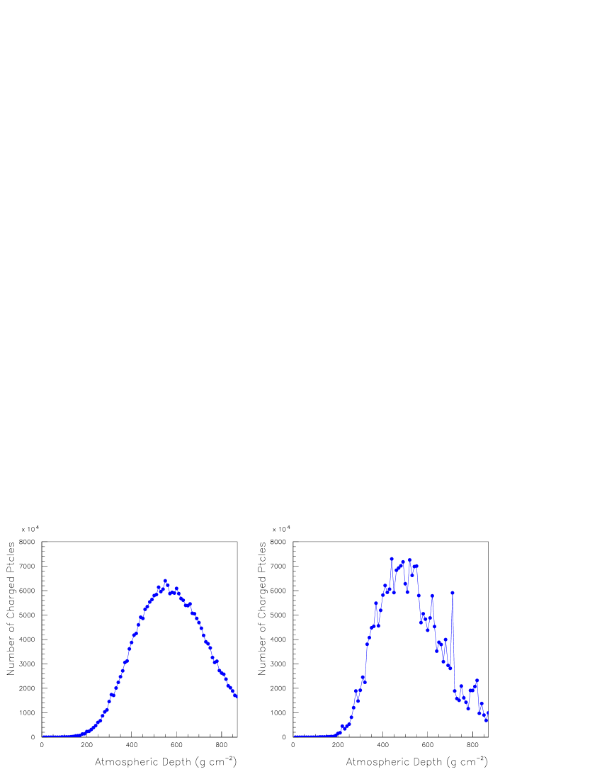
Figure 1: The longitudinal profiles of two simulated showers. At left the thinning level is $10^{-5.5}$ of primary energy, and at right $10^{-3.5}$.

To recover the depth of shower maximum from “noisy” thinned profiles it is customary to fit them to an empirical cascade shape function. This is also necessary when analyzing experimental data as the quality is often poor. The following function was introduced by Gaisser and Hillas [14] as a “simple analytic parameterization” of the longitudinal profile of air showers:

$$N(X)=N_{max}\left(\frac{X}{X_{max}}\right)^{X_{max}/\lambda}\exp{(X_{max}-X)/\lambda},$$ (1)

where $X$ is the atmospheric depth (in g cm^-2), $N_{max}$ is the number of cascade particles at shower maximum, $X_{max}$ is the depth of maximum, and $\lambda$ is a characteristic length parameter (in the above reference fixed at 70 g cm^-2). This is a Gamma Function, a form which naturally arises in cascade theory, and assumes that the first interaction is at $X=0$.

A fourth parameter $X_{0}$ is often introduced into Equation 1, ostensibly to allow for a variable first interaction point,

$$N(X)=N_{max}\left(\frac{X-X_{0}}{X_{max}-X_{0}}\right)^{(X_{max}-X_{0})/\lambda}\exp{(X_{max}-X)/\lambda}.$$ (2)

This seems somewhat inelegant as varying $X_{0}$ does not correspond to a translation along the $X$ axis, unless $X_{max}$ is also changed. The following (equivalent) form is physically clearer, where $X_{rise}$ is the distance from first interaction to shower maximum,

$$N(X)=N_{max}\left(\frac{X-X_{0}}{X_{rise}}\right)^{X_{rise}/\lambda}\exp{(X_{rise}+X_{0}-X)/\lambda}.$$ (3)

In practice, when fitting simulated hadronic cascade profiles to either Equation 2 or 3, it turns out that $X_{0}$ correlates poorly with the actual depth of first interaction, and frequently takes unphysical negative values. Experiments were made performing the fit with $X_{0}$ fixed at the actual depth of first interaction $X_{1}$. This produces a significantly poorer goodness of fit, and reduces the $X_{max}$ results by $\leq 10$ g cm^-2. The choice of Equation 2 or 3 also influences the $X_{max}$ results. For the remainder of this paper, in the interests of compatibility with other published results, Equation 2 was used with all four parameters free. Note that $X_{0}$ is best regarded as simply an additional arbitrary shape parameter.

To determine an appropriate thinning level for this study, sets of 500 proton showers were generated and fit, at each of 5 thinning levels; $10^{-3.5}$, $10^{-4.0}$, $10^{-4.5}$, $10^{-5.0}$ and $10^{-5.5}$. Taking the $10^{-5.5}$ thinned distributions as reference, a Kolmogorov test was performed on each of the more heavily thinned sets, and for each of the fit parameters. This is a statistical test of the compatibility in shape between two histograms — it yields the probability that they are drawn from the same parent distribution. All the fit parameters returned a high probability at thinning levels of $10^{-5.0}$ and $10^{-4.5}$, i.e. the results are indistinguishable within the statistics of a 500 event set. $X_{max}$ itself is extraordinarily robust, remaining unbiased even at $10^{-3.5}$ thinning. To be conservative a value of $10^{-4.5}$ was selected for the main study.

The compatibility of the parameter distributions was also checked when varying the zenith angle of the primary from 0 to 60 deg. $X_{max}$ was unaffected, but interestingly $N_{max}$ showed a small systematic increase with angle [7].

3 $X_{max}$ Results

3.1 Mean value of $X_{max}$

For the main study sets of 500 events were run at 14 half decade energy steps between $10^{14}$ and $10^{20.5}$ eV, with the 4 combinations of framework program and high energy hadronic interaction model given in Table 1. Sets were generated with both proton and iron nucleus primaries. This gives $500\times 14\times 4\times 2=56,000$ showers. The showers were run at a thinning level of $10^{-4.5}$ of primary energy, and a zenith angle of 45 deg. The resulting profiles were fit to Equation 2. Figure 2 shows the mean value of $X_{max}$ plotted against energy over the complete range; numerical values are given in Table 3. MOCCA-SIBYLL and CORSIKA-SIBYLL proton results are in good agreement, and the iron results are also close. This is very encouraging — the framework programs are complex and entirely independent — nevertheless they produce the same result. At higher energies the older MOCCA-Internal model diverges strongly to deeper $X_{max}$. CORSIKA-QGSjet produces much shallower results than SIBYLL at all energies; so much so that at $10^{20.5}$ eV MOCCA-Internal iron is equal to CORSIKA-QGSjet proton.

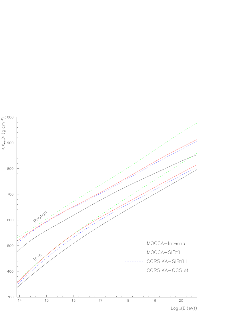
Figure 2: The mean depth of shower maximum versus energy for proton and iron primaries, and four program-frame / interaction-model combinations.

Figure 3 shows a comparison between published mean $X_{max}$ data from two experiments and the CORSIKA calculations. The data for $E<10^{17}$ eV are from the BLANCA experiment [3], and for $E>10^{17}$ eV from the Fly’s Eye [4]. The Fly’s Eye data contains a small un-corrected experimental bias, the removal of which would shift the lower energy points higher in the atmosphere by around 20 g cm^-2 [17]. Both SIBYLL and QGSjet are consistent with the data, in that the value remains within the proton-iron bounds. Also the general trends in composition versus energy are the same under the two models, although the absolute value and size of the changes differ. There is some evidence at $\sim 10^{16}$ eV that QGSjet is a more realistic model than SIBYLL [3, 18]; the extrapolation to the highest energies in both models must be regarded as tentative at best.

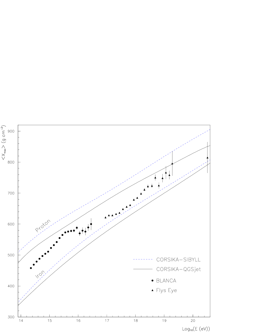
Figure 3: A Comparison of experimental mean $X_{max}$ data with simulations using two high energy hadronic interaction models.

3.2 Influence of the First Interaction on $X_{max}$

Why do the results shown in Figure 2 differ between the models? The proton-air cross sections used by SIBYLL and QGSjet are sufficiently similar that the mean free paths differ by $<5$ g cm^-2 over the complete energy range. This is to be compared to the 30–50 g cm^-2 difference in mean $X_{max}$.

When investigating the way in which the first interaction controls $X_{max}$ it is natural to subtract out the position of the first interaction; $X_{rise}=X_{max}-X_{1}$. Elasticity is defined as the energy fraction of the most energetic secondary. Normally a large fraction of the primary energy continues in the form of a “leading nucleon” and the remainder is split between many secondary pions and nucleons. Figure 4 shows $X_{rise}$ versus first interaction elasticity at $10^{19}$ eV. For events where the first interaction is catastrophic (small elasticity), the resulting shower takes fewer generations to reach maximum, and the correlation is strong. As elasticity becomes larger, the first interaction is no longer the controlling factor, and the relationship weakens. Interestingly, both models exhibit approximately the same correlation between elasticity and $X_{rise}$.

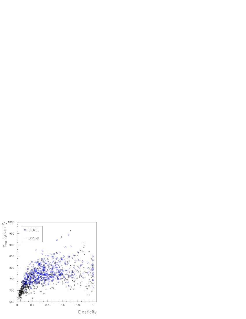
Figure 4: The correlation of $X_{rise}$ with first interaction elasticity for primary protons at $10^{19}$ eV.

Figure 5 shows the elasticity distributions versus energy. The reason the models produce different mean $X_{max}$ values is primarily because of their different elasticity distributions; QGSjet produces many more “hard” events, which lead to less deeply penetrating showers. SIBYLL has rather constant behaviour versus energy, while QGSjet is a more radical model, showing a stronger change; this is why the corresponding mean $X_{max}$ results diverge with increasing energy.

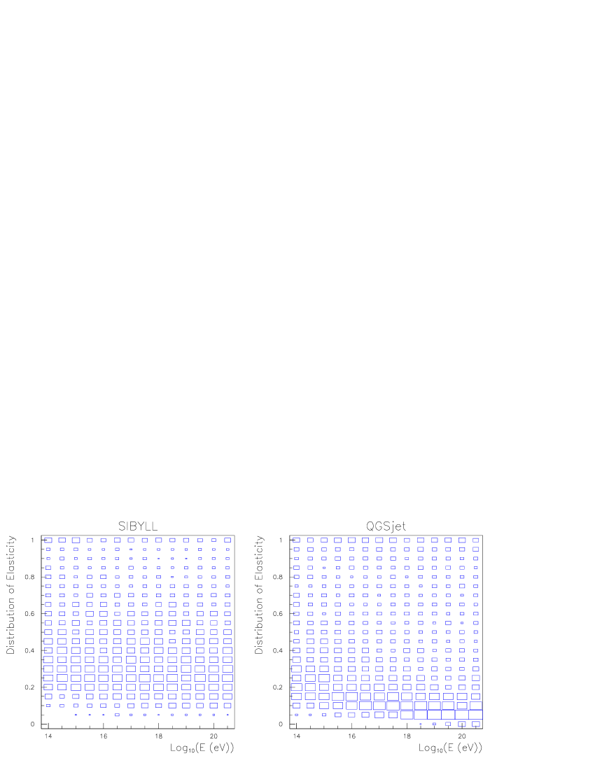
Figure 5: Elasticity of proton-air interactions versus energy for two models. The side length of the boxes is proportional to the bin contents.

Hadronic interactions models are complex and esoteric, with many parameters which can potentially be compared. The significance of Figure 4 is the realization that, for calculations of $X_{max}$ at least, the most important characteristic is also a very simple one: how much of the primary energy is expended in the first interaction?

3.3 Distribution of $X_{max}$

In Figure 2 it can be seen that QGSjet predicts that the difference between proton and iron mean $X_{max}$ decreases significantly with energy. However, the fluctuations do not decrease correspondingly, and the proton and iron distributions overlap to an increasing extent. If this model is correct, greater experimental statistics would be required to determine the mean composition with given accuracy. The situation is illustrated in Figure 6 where the bands contain 68% of the data (i.e. spanning the 16% and 84% points of the integral distribution). CORSIKA-SIBYLL shows stronger separation improving with increasing energy, while CORSIKA-QGSjet has weaker separation degrading with energy.

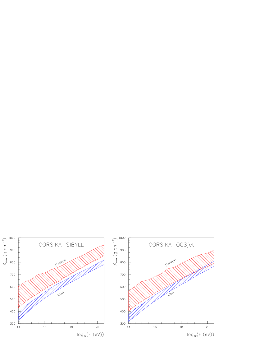
Figure 6: The distribution of $X_{max}$ versus energy shown as a band containing the central 68% of the distribution.

Proton primaries are deflected less by magnetic fields than more highly charged particles of the same total energy. It has been suggested that attempts to locate the origin of the highest energy cosmic rays, by studying their arrival directions, could be enhanced by making cuts on composition sensitive parameters, to increase the fraction of protons in the data sample. This would clearly work much less well if QGSjet is a more realistic model than SIBYLL.

For proton primaries the distribution of $X_{max}$ is strongly asymmetric, with a tail to deep $X_{max}$. This is presumably the result of fluctuations in the first interaction point, and is therefore connected to the proton-air cross section, which is a quantity of fundamental interest. Earlier simulations have suggested that,

$$\Lambda=c\>\lambda_{p-air},$$ (4)

where $\Lambda$ is the exponential slope, or “decrement”, of the trailing edge of the $X_{max}$ distribution, $\lambda_{p-air}$ is the proton-air mean free path, and $c$ is a constant of proportionality with a value between 1.2 and 1.6 dependent on hadronic interaction model [19].

The $X_{max}$ distributions were fit to an exponential starting at 100 g cm^-2 beyond the peak. An example distribution, with the fit, is shown in Figure 7. To avoid biasing the results it is essential to use a maximum likelihood algorithm since the bins on the far tail necessarily contain few events. Figure 8 shows the value of the ratio $c$, plotted versus energy, for one of the models. Testing each set of results against the hypothesis of energy independence yields the values given in Table 2. With the available statistics, the reduced $\chi^{2}$ numbers show little evidence for energy dependence. The SIBYLL based models give values close to $1.15$, while the other two are around $1.30$; this difference appears to have significance.

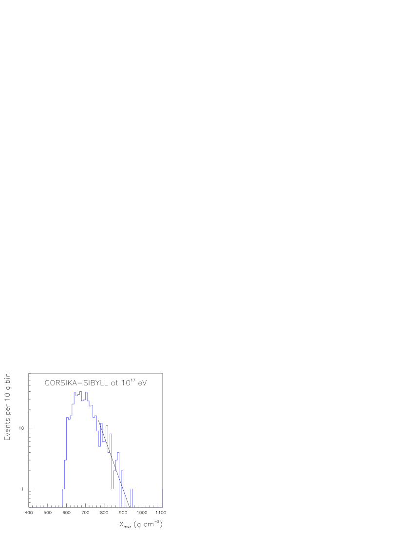
Figure 7: An example $X_{max}$ distribution with exponential trailing edge fit.

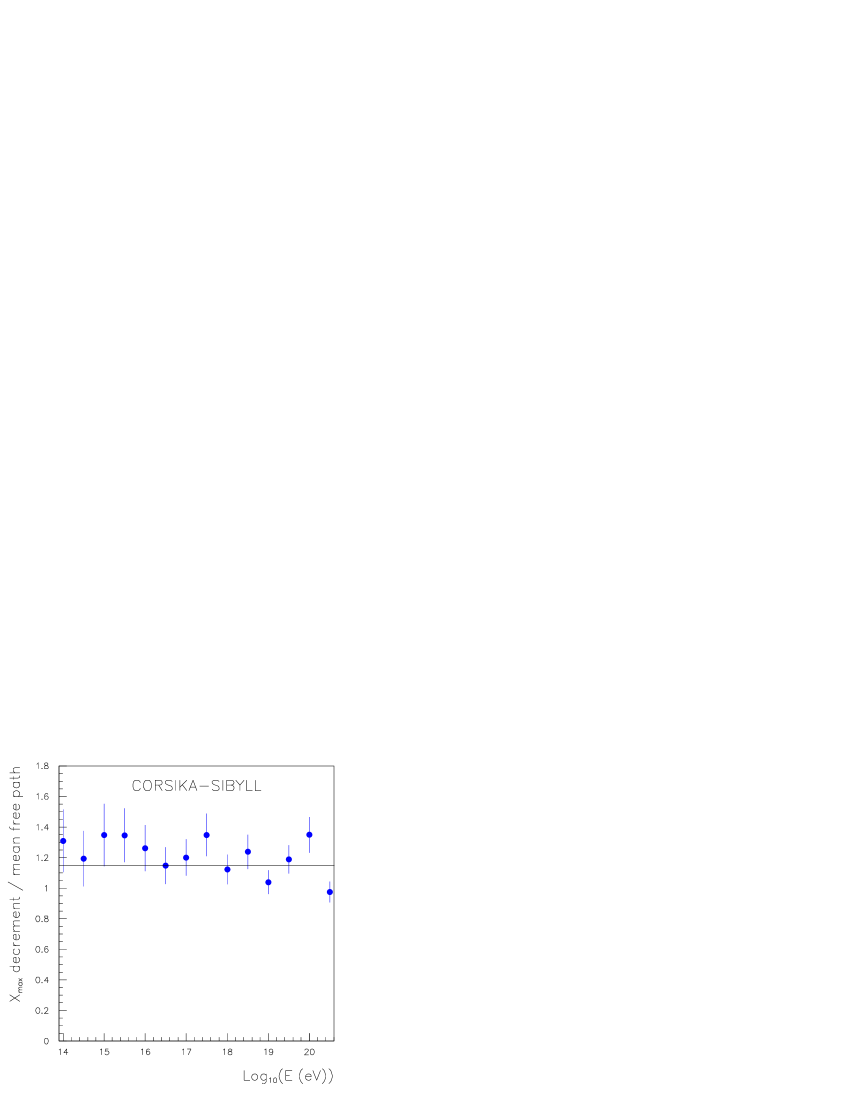
Figure 8: Ratio $c$ plotted versus energy. The most probable value is shown as a horizontal line.

Model	Ratio $c$	$\chi^{2}/ndf$
MOCCA-Internal	$1.32\pm 0.03$	0.77
MOCCA-SIBYLL	$1.16\pm 0.03$	1.24
CORSIKA-SIBYLL	$1.15\pm 0.03$	1.38
CORSIKA-QGSjet	$1.30\pm 0.04$	0.43

Table 2: Decrement / mean-free-path data.

4 Conclusions

When running shower simulations to study $X_{max}$ it is better to generate heavily thinned showers, with explicit low energy hadronic and electromagnetic cascades, than to rely on analytic approximations for these parts of the calculation. The latter has frequently been done in the past, leading to concerns that the results are biased to an unknown extent. When working with an explicit, but thinned, cascade simulation it is possible to determine an appropriate thinning level empirically, by comparing against more lightly thinned results.

Carefully calculated $X_{max}$ results have been presented, over a wide energy range, for proton & iron primaries, using four combinations of framework program and high energy hadronic interaction model. It is hoped that these will be of use for future comparisons with experimental data, and with other simulation results.

The way in which the first interaction controls $X_{max}$ has been investigated. The influence is strong — if one were to use model $A$ for the first few interactions, and model $B$ thereafter, the mean $X_{max}$ results would be close to using model $A$ throughout. QGSjet predicts that the separation between proton and iron $X_{max}$ declines at the highest energies. If this is true it is unfortunate from an experimental perspective.

It would be very useful if a common reference set of showers were made available by the authors of new, or modified, hadronic interaction models. For the purposes of longitudinal profile comparison the set used here seems adequate; the raw and processed output is available online [20].

The Fermilab computing department are thanked for the use of their machines.

Primary	$\log_{10}(E(eV))$	$<\!X_{max}\!>$, $\sigma X_{max}$ (g cm-2)
		MOCCA		CORSIKA
		Internal	SIBYLL	SIBYLL	QGSjet
Proton	14.0	537 , 96	525 , 91	517 , 97	484 , 96
	14.5	570 , 86	559 , 92	560 , 99	525 , 92
	15.0	605 , 78	597 , 86	589 , 97	560 , 88
	15.5	637 , 72	625 , 81	621 , 84	587 , 76
	16.0	674 , 71	651 , 72	651 , 81	618 , 72
	16.5	704 , 62	676 , 59	679 , 70	646 , 70
	17.0	738 , 60	713 , 65	699 , 63	679 , 75
	17.5	767 , 54	733 , 57	729 , 63	705 , 68
	18.0	802 , 53	765 , 60	762 , 59	728 , 69
	18.5	839 , 50	793 , 53	790 , 62	755 , 67
	19.0	867 , 44	829 , 55	817 , 52	779 , 68
	19.5	908 , 60	852 , 49	847 , 52	804 , 68
	20.0	940 , 50	883 , 53	875 , 54	825 , 59
	20.5	972 , 42	908 , 47	900 , 45	849 , 59
Iron	14.0	370 , 36	366 , 38	357 , 32	346 , 32
	14.5	420 , 34	414 , 35	407 , 33	390 , 30
	15.0	461 , 34	464 , 34	452 , 31	432 , 29
	15.5	507 , 32	508 , 34	493 , 28	471 , 26
	16.0	545 , 29	542 , 31	533 , 27	509 , 25
	16.5	582 , 25	577 , 27	568 , 27	544 , 26
	17.0	619 , 23	610 , 29	600 , 25	577 , 24
	17.5	652 , 22	641 , 26	631 , 25	609 , 22
	18.0	688 , 21	668 , 24	660 , 25	640 , 24
	18.5	720 , 18	697 , 21	689 , 24	669 , 23
	19.0	754 , 18	725 , 22	717 , 21	701 , 20
	19.5	787 , 17	754 , 21	744 , 20	730 , 21
	20.0	820 , 16	783 , 19	774 , 20	759 , 21
	20.5	853 , 14	809 , 19	802 , 20	791 , 22

Table 3: Mean and standard deviation values of $X_{max}$ for proton and iron primaries, and four program-frame / interaction-model combinations. Each pair of numbers comes from a 500 shower set.

References

- [1] S.P. Swordy and D.B. Kieda, Astropart. Phys. 13 (2000) 137. Preprint astro-ph/9909381.
- [2] F. Arqueros et al., accepted in Astron. Astrophys. (1999). Preprint astro-ph/9908202.
- [3] J.W. Fowler et al., submitted to Astropart. Phys. (2000). Preprint astro-ph/0003190.
- [4] D.J. Bird et al., Phys. Rev. Lett. 71 (1993) 3401.
- [5] T. Abu-Zayyad et al., submitted to Nucl. Instr. Meth. in Phys. Res. A (1999).
-
[6]
The Auger Collaboration,
Design Report,
FNAL (1997).
Available from
http://www.auger.org/admin/DesignReport -
[7]
C. Pryke,
Auger Project Report GAP-98-035.
Available from
http://aupc1.uchicago.edu/~pryke/auger/documents/ - [8] A.M. Hillas, Nuc. Phys. B (Proc. Suppl.) 52B (1997) 29.
- [9] R.S. Fletcher et al., Phys. Rev. D 50 (1994) 5710.
-
[10]
J. Knapp et al,
Reports FZKA 6019 and FZKA 5828 (1998 and 1996),
Forschungszentrum Karlsruhe.
Available from
http://www-ik3.fzk.de/~heck/corsika/ - [11] N.N. Kalmykov et al., Nuc. Phys. B (Proc. Suppl.) 52B (1997) 17.
- [12] W.R Nelson, H. Hirayama, D.W.O. Rogers, Report SLAC 265 (1985), Stanford Linear Accelerator Center.
- [13] H. Fesefeldt, Report PITHA-85/02 (1985), RWTH Aachen.
- [14] T.K. Gaisser and A.M. Hillas, Proc. 15th Int. Cosmic Ray Conf. (Plovdiv), 8 (1977) 353.
- [15] M. Goosens et al., HBOOK Reference Manual, CERN, Geneva Switzerland, (1995) page 103.
- [16] T. Abu-Zayyad et al., submitted to Phys. Rev. Lett. (1999). Preprint astro-ph/9911144.
- [17] T.K. Gaisser et al., Phys. Rev. D 47 (1993) 1919.
- [18] T. Antoni et al., J. Phys. G: Nucl. Part. Phys. 25 (1999) 2161.
- [19] R.W. Ellsworth et al., Phys. Rev. D 26 (1982) 336.
-
[20]
ftp://aupc1.uchicago.edu/pub/auger/showlib/modcomp/.