The violent past of Cygnus X–2

Abstract

Cygnus X–2 appears to be the descendant of an intermediate–mass X–ray binary (IMXB). Using Mazzitelli’s (1989) stellar code we compute detailed evolutionary sequences for the system and find that its prehistory is sensitive to stellar input parameters, in particular the amount of core overshooting during the main–sequence phase. With standard assumptions for convective overshooting a case B mass transfer starting with a $3.5{\rm M_{\odot}}$ donor star is the most likely evolutionary solution for Cygnus X–2. This makes the currently observed state rather short–lived, of order 3 Myr, and requires a formation rate $>10^{-7}-10^{-6}$ yr^-1 of such systems in the Galaxy. Our calculations show that neutron star IMXBs with initially more massive donors ($\ga 4{\rm M_{\odot}}$) encounter a delayed dynamical instability; they are unlikely to survive this rapid mass transfer phase. We determine limits for the age and initial parameters of Cygnus X–2 and calculate possible dynamical orbits of the system in a realistic Galactic potential, given its observed radial velocity. We find trajectories which are consistent with a progenitor binary on a circular orbit in the Galactic plane inside the solar circle that received a kick velocity $\leq 200$ km s^-1 at the birth of the neutron star. The simulations suggests that about $7\%$ of IMXBs receiving an arbitrary kick velocity from a standard kick velocity spectrum would end up in an orbit similar to Cygnus X–2, while about $10\%$ of them reach yet larger Galactocentric distances.

1 Introduction

The $9.84$ d period neutron–star binary Cygnus X–2 has long been regarded as an archetypal long–period low–mass X–ray binary (Cowley et al. 1979, Webbink et al. 1983) where nuclear expansion of a Hayashi line giant drives mass transfer. Yet recent optical photometry and high–resolution spectroscopy, while confirming that the donor has a low mass (Casares et al. 1998; Orosz & Kuulkers 1999), unambiguously showed that the spectral type of the optical counterpart is A$5\pm 2$ (Casares et al. 1998), significantly too hot for a Hayashi line donor.

King & Ritter (1999; hereafter KR) and Podsiadlowski & Rappaport (2000; PR) argued that the system must be the descendent of an intermediate–mass X–ray binary (IMXB), with $3-4{\rm M_{\odot}}$ as the likely initial donor mass. Such systems undergo a rapid mass transfer phase, previously regarded as fatal, with transfer rates exceeding the Eddington value by several orders of magnitude. For a narrow range of initial separations the systems never reach the Hayashi line, or evolve away from it, during the subsequent phase with slower mass transfer.

KR suggested that Cygnus X–2 is the product of a “case B” mass transfer sequence, where the donor star was already expanding towards the giant branch when mass transfer began (Kippenhahn & Weigert [1967]). By contrast, PR preferred an evolution where mass transfer started while the donor was still on the main sequence, with core hydrogen burning terminating during the mass transfer phase. KR’s considerations are semi–analytical and entirely based on generalised main–sequences (Giannone et al. 1968), while PR performed detailed binary sequences with a full stellar code. In Sect. 2 and 3 we use our evolutionary code to reexamine critically the case B solution rejected by PR, and resolve the discrepancy between KR and PR. To see how common a Cygnus X–2–like evolution is we consider IMXBs with still higher initial donor masses in Sect. 4.

A further peculiarity of Cygnus X–2, addressed in Sect. 5, is its dynamical state. The system has a measured line-of-sight velocity of -208.6 km/s (Casares et al. 1998) and a Galactic latitude of -11.32^∘ and longitude of 87.33^∘. At a distance of 11.6 kpc from the sun (Smale 1998), this places Cygnus X–2 at a Galactocentric distance of 14.2 kpc, and a distance from the Galactic plane of 2.28 kpc. Integrating the equations of motion in the Galactic potential we use Monte Carlo techniques to investigate possible trajectories of Cygnus X–2.

2 Constraining the prehistory of Cygnus X–2

The observed location of the donor star of Cygnus X–2 in the middle of the Hertzsprung gap in the HR diagram, and its small mass ($0.4-0.7{\rm M_{\odot}}$), suggest that the mass of the hydrogen–rich envelope remaining above the donor’s helium core is very small ($M_{\rm H}/M_{\rm He}\la 0.05$). Stars with an initial mass $3-4.5{\rm M_{\odot}}$ leave the core hydrogen burning phase with a helium core mass $M_{\rm He}$ in this range (e.g. Bressan et al. 1993). Mass transfer from such an intermediate–mass star on to a less massive neutron star is thermally unstable and involves an initial phase of rapid mass transfer with a highly super–Eddington transfer rate. This rapid phase lasts roughly until the mass ratio is reversed and the donor’s Roche lobe expands upon further mass transfer. The subsequent slower transfer phase proceeds on the donor’s thermal timescale, which is essentially given by the Kelvin–Helmholtz time of the donor when it left the main sequence.

PR identified two possible routes from the post–supernova binary, i.e. after the formation of the neutron star, to the present system configuration. One route is via a genuine case B evolution, the other via an evolution they labelled ‘case AB’. In the former the donor star has already left the main sequence when it fills its Roche lobe for the first time. The mass transfer phase is short–lived, with most of the mass transferred at a highly super–Eddington rate. Hence the neutron star mass increase is negligible, even if it accretes at the Eddington rate during the whole evolution. In the case AB solution discussed by PR mass transfer already starts during the donor’s main–sequence phase. The system briefly detaches when core hydrogen burning terminates, but mass transfer resumes when shell–burning is well established. As the rapid mass transfer phase terminates before the donor leaves the main sequence the subsequent slow phase proceeds on a much longer timescale than in the genuine case B solution — the thermal time of the now less massive donor at the terminal main–sequence. The transfer rate is sub–Eddington for some time and the neutron star grows in mass.

Given this we explore three different prescriptions to project the evolution of Cygnus X–2 backwards in time:

(Model 1) To represent a case B evolution we assume that $M_{1}=$const., and that any material lost from the system carries the specific orbital angular momentum of the neutron star. Then the initial orbital separation $a_{i}$ is

$$a_{i}=a\,\frac{M_{1}+M_{2}}{M_{1}+M_{2i}}\left(\frac{M_{2}}{M_{2i}}\right)^{2}\exp\left(\frac{2(M_{2i}-M_{2})}{M_{1}}\right),$$ (1)

where $M_{2i}$, $M_{2}$ denote the initial and present donor mass, and $a$ the present separation (e.g. KR). This solution is valid only if $a_{i}>a_{\rm TMS}$, the orbital separation of a binary with a Roche–lobe filling terminal main–sequence (TMS) star of mass $M_{2,i}$.

(Model 2) The same applies to a case AB evolution, except that we require $a_{i}<a_{\rm TMS}$.

(Model 3) To account for a possible prolonged phase with sub–Eddington mass transfer in a case AB sequence we allow mass transfer to be conservative (total binary mass and orbital angular momentum is constant) for the last part of the evolution. We assume that the neutron star mass at birth was $1.4\,{\rm M_{\odot}}$, and that the present neutron star mass is $>1.4\,{\rm M_{\odot}}$. Hence the evolution backwards in time consists of two branches. During the conservative phase, characterised by $aM_{1}^{2}M_{2}^{2}=$constant, $M_{1}$ reduces from its present value to $1.4\,{\rm M_{\odot}}$. The second phase is calculated with constant neutron star mass ($1.4{\rm M_{\odot}}$), as in models 1 and 2 above.

The present system parameters of Cygnus X–2 are: orbital period $P_{0}=9.844$ d, mass ratio $q=0.34\pm 0.04$ (Casares et al. 1998), and neutron star mass $M_{1}=1.4-1.8{\rm M_{\odot}}$. This mass range accommodates the canonical neutron star mass at birth, as well as the estimate by Orosz & Kuulkers (1999) based on modelling the observed ellipsoidal variations. If we adopt a specific value $M_{1}$ for the present neutron star mass, then the present donor mass is constrained to the range $0.30M_{1}\la M_{2}\la 0.38M_{1}$ by the observed mass ratio. This translates into a range of allowed initial separations, as shown by the hatched regions in Fig. 1, for case B (model 1, wide spacing) and case AB (model 2, narrow spacing) evolution. The parameter space for case AB solutions with model 3 assumptions is tiny and hence not shown in the figure. For conservative mass transfer (model 3) the orbital separation of Cygnus X–2 today increases less steeply with decreasing donor mass than for the isotropic wind case (model 2). Hence the separation for model 3 sequences describing the past evolution of Cygnus X–2 is generally larger than for the corresponding model 2 sequences. In particular, model 3 solutions require larger initial separations. Most of them are in conflict with the limit $a_{i}<a_{\rm TMS}$, i.e. inconsistent with the assumption that the donor was on the main sequence when mass transfer started.

More generally, if the mass lost from the system in sequences with $M_{1}=$ const. carries more (less) specific angular momentum than that of the neutron star, the required initial separation is larger (smaller) than estimated by (1). A somewhat higher loss seems more likely than a smaller loss, hence this reduces the parameter space available for case AB solutions.

Even if Fig. 1 indicates a viable solution it is not clear if the corresponding evolutionary sequence reproduces Cygnus X–2. Although the donor will have the observed mass (and hence radius) at the observed orbital period $P_{0}$, the effective temperature is of course not constrained by the above considerations. To check this we need a detailed binary sequence with full stellar models, as presented in the next section. In particular, it appears that the case AB sequences described by PR require the donor star to be already fairly close to the end of core hydrogen burning at turn–on of mass transfer. This is likely to narrow the parameter space for case AB sequences even further.

We note that the limits shown in Fig. 1 depend via $a_{\rm TMS}$ somewhat on the stellar input physics, in particular on the amount of convective core overshooting (cf. the discussion in the next section).

Figure 1: Allowed range for the initial orbital separation $a_{i}$ as a function of initial donor mass $M_{2i}$, for three different fixed neutron star masses, as labelled. The hatched areas correspond to case B evolution (model 1; wide spacing) and case AB evolution (model 2; narrow spacing), assuming constant neutron star mass. The parameter space for case AB solutions with model 3 assumptions is so small that it is not shown. The almost horizontal boundary at $a_{i}=a_{\rm TMS}\mathrel{\raise 1.29167pt\hbox{$\sim$}\mkern-14.0mu\lower 1.72218pt\hbox{$-$}}11\,{R_{\odot}}$ separating case B and case AB solutions represents the terminal main sequence. $a_{\rm TMS}$ was calculated using main–sequence models by Dominguez et al. (1999). See text for details.

3 Model calculations

We calculated several detailed early massive case B binary evolution sequences, using Mazzitelli’s stellar code in its 1989 version (see Mazzitelli 1989, and references therein, for a summary of the input physics). Mass transfer was treated as in Kolb (1998). Table 1 summarises initial and final system parameters. The neutron star mass was $1.4{\rm M_{\odot}}=$ const. in each case, with angular momentum loss treated as in model 1 above. Specifically, we present in detail the evolution of a system with initial donor mass $M_{2}=3.5{\rm M_{\odot}}$ and orbital separation $a_{i}=13.3{R_{\odot}}$ (Sequence I) and $11.1{R_{\odot}}$ (sequence II).

The figures 2-4 confirm the general behaviour of case B evolutionary sequences as described above. Sequence I gets very close to the observed state of Cygnus X–2, although it fails to fit all observed parameters simultaneously with high accuracy. The evolutionary track in the HR diagram passes through the Cygnus X–2 error box, but at a period slightly longer than the observed value $P_{0}=9.844$ d. This can be seen in Fig. 4, which shows that at $P_{0}$ the sequence I donor is somewhat too cool, while in sequence II it is somewhat too hot. Hence the initial separation for a simultaneous fit of $P$, $T_{\rm eff}$ (and $L$) lies between $11.1{R_{\odot}}$ and $13.3{R_{\odot}}$. The transfer rate at $P_{0}$ for sequence I is $5\times 10^{-8}{\rm M_{\odot}{\rm yr}^{-1}}$, a factor $2-3$ higher than the Eddington rate.

Observational estimates place the actual accretion rate in Cygnus X–2 close to the Eddington limit. With no evidence of significant mass loss from the system we expect that the transfer rate is also of the order of the Eddington rate. As the transfer rate in the model sequence is set by the thermal time of the progenitor star, a somewhat smaller initial secondary mass (e.g. $3.0{\rm M_{\odot}}$) would give a lower rate; this has already been noted by PR.

We note the following main differences between our sequence I and the case B sequence calculated by PR:
(1) PR chose $21.3{R_{\odot}}$ as the initial separation. This leads to the combination $1.4+0.66{\rm M_{\odot}}$ for the component masses at $P=P_{0}$, i.e. to a mass ratio $0.47$, significantly larger than observed. Hence the PR case B sequence represents a poor fit for Cygnus X–2.
(2) More importantly, the mass transfer rate in the slow phase of sequence I decreases from $10^{-7}{\rm M_{\odot}{\rm yr}^{-1}}$ to $10^{-8}{\rm M_{\odot}{\rm yr}^{-1}}$ over a period of 2.5 Myr, while in PR’s model the transfer rate is always larger than $10^{-7}{\rm M_{\odot}{\rm yr}^{-1}}$ (which is inconsistent with observations). A similar calculation by Tauris et al. (2000) with essentially the same stellar code as the one used by PR gives a similarly high rate in the slow phase.

The initial separation for our sequence II is essentially the same as the one used by PR for their case AB evolution ($11.5{R_{\odot}}$, corresponding to a stellar radius $5.6{R_{\odot}}$ of the donor at turn–on of mass transfer). The most important difference between the two calculations is the degree of convective overshooting assumed during the main–sequence phase: none in our models, a very strong one in PR’s models. Hence PR’s main–sequence band is much wider, with $6.6{R_{\odot}}$ as the maximum radius $R_{2,\rm max}$ that a $3.5{\rm M_{\odot}}$ star reaches during core hydrogen burning, compared to $3.6{R_{\odot}}$ in our case. A moderate extent of core overshooting is favoured in the literature, giving $R_{2,\rm max}=5.0{R_{\odot}}$ (Schaller et al. 1992), $5.7{R_{\odot}}$ (Bressan et al. 1993) and $4.8{R_{\odot}}$ (Dominguez et al. 1999) for a $3.5{\rm M_{\odot}}$ star with solar composition. Schröder et al. (1997) — who use the same code and input physics as PR — prefer a rather efficient overshooting leading to values up to $R_{2,\rm max}=7.1{R_{\odot}}$, while in a subsequent paper (Pols et al. 1997) the same authors concluded that $R_{2,\rm max}=5.9{R_{\odot}}$ (which corresponds to their overshooting parameter $\delta=0.12$) provides the best overall fit to observations. This is only barely larger than the donor’s radius at turn–on of mass transfer in PR’s case AB solution. Hence standard assumptions about overshooting favour a case B solution for Cygnus X–2 over a case AB solution.

We conclude that a case B solution is a viable fit for the evolutionary history of Cygnus X–2. Given the parameter space limitations for a case AB evolution it does appear as the more likely solution for Cygnus X–2, even though this implies that the presently observed state of Cygnus X–2 is rather short–lived, of order several million years.

PR pointed out that the surface composition of the donor in Cygnus X–2 would be significantly hydrogen–depleted ($X\mathrel{\raise 1.29167pt\hbox{$\sim$}\mkern-14.0mu\lower 1.72218pt\hbox{$-$}}0.1$) and show signs of CNO–processing if it had undergone a case AB evolution. Unfortunately, this does not distinguish unambiguously between a case AB and case B evolution, as the same is in principle true for a donor that had undergone a case B mass transfer. The models in our sequence I close to the position of Cygnus X–2 have a surface hydogen mass fraction of $X=0.29$, while C/N and O/N are close to the equilibrium values for CNO burning at $2\times 10^{7}$ K.

$M_{2i}/{\rm M_{\odot}}$	$P_{i}/$d	$a_{i}/{R_{\odot}}$	$M_{2f}/{\rm M_{\odot}}$	$P_{f}/$d	comment
3.5	1.94	11.1	0.44	9.70	Sequence II
3.5	2.54	13.3	0.45	12.13	Sequence I
3.5	3.13	15.3	0.45	14.65
3.75	4.23	19.0	0.50	13.24
4.0	1.25	8.55	3.99	1.24	runaway
4.0	6.43	25.5	3.00	0.443	runaway
5.0	4.86	22.4	4.34	2.19	runaway

Table 1: Donor mass $M_{2f}$ and orbital period $P_{f}$ when mass transfer ceases for sequences with different initial donor mass $M_{2i}$ and initial orbital period $P_{i}$ (initial orbital separation $a_{i}$). Sequences labelled “runaway” encounter the delayed dynamical instability; $M_{2f}$ and $P_{f}$ refer to the system at this point.

Figure 2: HR diagram showing sequence I (solid) and a track of a $3.5{\rm M_{\odot}}$ single star (dotted), calculated without core overshooting. Labels along the track indicate the donor mass. The shaded error box marks the observed location of Cygnus X–2 (lower and upper bound correspond to donor masses $0.4{\rm M_{\odot}}$ and $0.7{\rm M_{\odot}}$, respectively).

Figure 3: Mass transfer rate $\dot{M}$ vs time (elapsed since the beginning of core hydrogen burning) for sequence I. Wiggles reflect numerical noise due to the explicit treatment of mass transfer. The instabilities are particularly strong at the end of the rapid phase close to $t=173.8$ Myr. The semi–regular dips of $\dot{M}$ during the slow phase are due to sudden changes of the stellar radius, caused by a discontinuous change of the inner boundary of the convective envelope.

Figure 4: Upper panel: Mass transfer rate $\dot{M}$ vs orbital period $P$ for sequence I. The numerical noise at the end of the rapid phase ($7<P/{\rm d}<8$) is suppressed. The dotted vertical line marks the period of Cygnus X–2. Lower panel: Effective temperature vs $P$, for sequence I (solid) and II (dashed). The filled and open circle on the tracks mark where the donor mass is $0.6{\rm M_{\odot}}$ and $0.5{\rm M_{\odot}}$, respectively. The short bar indicates the location of Cygnus X–2.

4 Sequences with initially more massive donor stars

The calculations discussed so far represent early case B mass transfer solutions for systems with a moderate initial mass ratio, $q=M_{2}/M_{1}\ga 2.5$. Systems with smaller mass ratio ($q\la 1$) have no initial rapid mass transfer phase and can be understood semi–analytically (see e.g. Kolb 1998, Ritter 1999), while the fate of systems with yet larger initial mass ratio $\ga 3$ is unclear. Hjellming (1989) pointed out that sustained thermal–timescale mass transfer can lead to a delayed transition to dynamical–timescale mass transfer. The reason for this is that the adiabatic mass–radius index of initially radiative stars decreases significantly when the radiative envelope is stripped rapidly. This causes the Roche lobe to shrink faster than the star. Estimates for the critical initial mass ratio which just avoids the delayed dynamical instability give $q\mathrel{\raise 1.29167pt\hbox{$\sim$}\mkern-14.0mu\lower 1.72218pt\hbox{$-$}}3-4$ (Hjellming 1989; Kalogera & Webbink 1996), although none of these are based on self–consistent mass transfer calculations.

This critical value is relevant for identifying possible descendants of neutron–star systems undergoing early massive case B mass transfer. These should appear as binary millisecond pulsars lying significantly below the orbital period–white dwarf mass relation found by Rappaport et al. (1995; see also Tauris & Savonije 1999 for calculations with updated input physics) for systems descending from Hayashi line low–mass X–ray binaries. Obvious candidates are systems with a fairly high–mass white dwarf but short orbital period. The most discrepant system is B0655+64 ($P=1.03$ d, $M_{\rm WD}\ga 0.7$; cf. KR). The fairly massive white dwarf implies a donor mass $\ga 5{\rm M_{\odot}}$ in the progenitor binary.

We performed test calculations similar to our sequences I and II, but with initial donor mass $3.75{\rm M_{\odot}}$, $4.0{\rm M_{\odot}}$ and $5.0{\rm M_{\odot}}$. While the $3.75{\rm M_{\odot}}$ sequence was stable throughout, the $4.0{\rm M_{\odot}}$ and $5.0{\rm M_{\odot}}$ sequences encountered runaway mass transfer (where we stopped the calculations) rather early in the rapid mass transfer phase (see Tab.1). An additional test sequence with a $3{\rm M_{\odot}}$ donor near the end of core hydrogen burning and initial mass ratio 4 (i.e. primary mass $0.75{\rm M_{\odot}}$, assumed constant, as above) encountered runaway mass transfer at a donor mass $2.6{\rm M_{\odot}}$. This is in perfect agreement with Hjellming’s prediction, based on his Fig. IV.1 and a Roche lobe curve corresponding to $q=4$.

Unless a neutron star binary can survive even such a dynamical–timescale mass transfer, the phase space available for a Cygnus X–2–like evolution is severely limited by this upper limit on the initial donor mass. Our calculations suggest that if most neutron stars form with $1.4{\rm M_{\odot}}$ the maximum white dwarf mass in an endproduct of early massive case B evolution is $\la 0.55{\rm M_{\odot}}$. If this is true, neither B0655+64 nor the recently discovered system J1453-58 ($P=12.422$ d, $M_{\rm WD}\ga 0.88{\rm M_{\odot}}$; cf. Manchester et al. 1999) can have formed in this way.

The occurrence of the delayed dynamical instability is intimately linked to the internal structure of the donor star. Therefore it is not surprising that the maximum initial donor mass for early case B mass transfer, just avoiding this instability, depends on the stellar input physics. Using an updated version of Eggleton’s stellar code (see e.g. Tauris & Savonije 1999), Tauris et al. (2000) found $5\,{\rm M_{\odot}}$ for this limit, with a corresponding maximum white dwarf mass $0.8\,{\rm M_{\odot}}$ in millisecond pulsar binaries formed in this way.

5 The trajectory of Cygnus X–2

As described in the introduction, Cygnus X–2 is in an unusual dynamical state. In this section we investigate possible trajectories of Cygnus X–2, given the observed line–of–sight velocity and the constraints on the evolutionary state as derived in Secs. 2 and 3.

In Fig. 5 we plot the cumulative velocity distribution for systems with initial separations of $d=15R_{\odot}$, i.e. immediately after circularisation of the binary orbit following the SN explosion producing the neutron star. The secondary is taken to have a mass $M_{2}=3.5$ M_⊙ while the mass of the helium star prior to the supernova is $M_{1}=5.0$ M_⊙. We consider two different distributions for the kick velocity imparted to the neutron star; namely those by Hansen & Phinney (1997) and Fryer (1999). Throughout the following section, when we refer to kick velocities we mean the kick imparted on the binary allowing for the effects of mass–loss and an asymmetric supernova, and not simply the kick imparted on the neutron star from the latter.

Given its present position and velocity, we integrate the trajectory of Cygnus X–2 backwards to the birth of the neutron star using a model for the Galactic potential suggested by Paczyński (1990) (reviewed in the Appendix). From sections 2 and 3 it is clear that the age $t$ of the neutron star is essentially the main–sequence lifetime of the progenitor star of the present donor. To account for the allowed range of the initial donor mass and for uncertainties from the width of the main–sequence we choose $150<t/{\rm Myr}<275$. As only the line-of-sight velocity, ${\bf v}_{los}$, is known, we considered a set of trajectories where the current velocity was given by

$${\bf v}={\bf v}_{\odot}+{\bf v}_{los}+\alpha{\bf v}_{1}+\beta{\bf v}_{2}$$ (2)

where ${\bf v}_{los}$, ${\bf v}_{1}$, and ${\bf v}_{2}$ are mutually orthogonal, and ${\bf v}_{1}$ has a zero component in the $z$ direction. When computing trajectories, it is most convenient to work in units related to the mass and size of the galaxy. As a natural unit of velocity we use 207 km/s, the Kepler velocity at 1 kpc distance from a point mass $10^{10}$ M_⊙. In the above equation ${\bf v}_{1}$, and ${\bf v}_{2}$ are given unit lengths in our code units.

Figure 5: The cumulative velocity distribution (in km/s) for systems with initial separations, $d=15R_{\odot}$. This is the velocity of the centre–of–mass of the binary as opposed to the kick of the neutron star itself. Dotted line is computed from the neutron star kick distribution of Hansen & Phinney (1997), whereas the dashed line is for the kick distribution of Fryer (1999).

Figure 6: The kick velocity, $V_{\rm k}$ (in km/s), of binaries as a function of formation radius, $r$ (in kpc). In the case of the larger dots, $150<t<275$, and $5<r<10$.

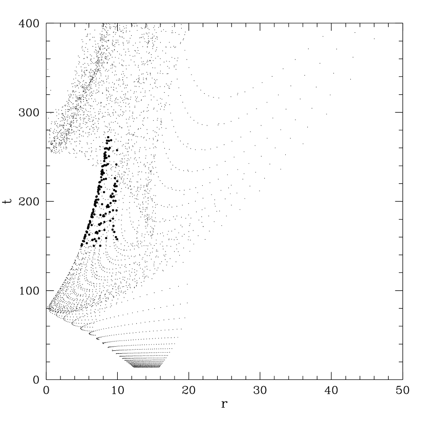
Figure 7: The age of formation, $t$ (in Myr), of binaries as a function of formation radius, $r$ (in kpc). For the larger dots, $150<t<275$, and $V_{\rm k}\leq 200$ km/s.

We integrated the equations (A9) for a range of values of $\alpha$ and $\beta$ and noted the radius, $r$, and time, $t$, whenever the trajectory cut the Galactic plane. We also computed the kick velocity, $V_{\rm k}$ the system must have had if the neutron star has formed at that time, assuming the system had previously been in a circular orbit in the Galactic plane.

In Fig. 6 we plot the values of $r$ and $V_{\rm k}$ for all values of $\alpha$ and $\beta$. We note that for $r\mathrel{\raise 1.29167pt\hbox{$<$}\mkern-14.0mu\lower 2.58334pt\hbox{$\sim$}}10$ kpc, 140 km/s $\mathrel{\raise 1.29167pt\hbox{$<$}\mkern-14.0mu\lower 2.58334pt\hbox{$\sim$}}V_{\rm k}\mathrel{\raise 1.29167pt\hbox{$<$}\mkern-14.0mu\lower 2.58334pt\hbox{$\sim$}}$ 600 km/s. This range of required values of $V_{\rm k}$ should be compared with that expected given the neutron star kick distributions of Hansen & Phinney (1997) and Fryer (1999) in Fig. 5. It is clear from Fig. 5 that the expected value of $V_{\rm k}$ is far lower than that required for many of the trajectories shown in Fig. 6. In other words, in a large fraction of systems formed at a radius $r\mathrel{\raise 1.29167pt\hbox{$<$}\mkern-14.0mu\lower 2.58334pt\hbox{$\sim$}}10$ kpc, the trajectory of the binary will confine the system to the inner regions of the Galaxy; Cygnus X–2 must have been relatively unusual in reaching out beyond the solar circle.

We plot the time of formation, $t$, as a function of $r$ for all values of $\alpha$ and $\beta$ in Fig. 7. As in Fig. 6, the data points where $150$ Myr $<t<275$ Myr and $V_{k}\leq 200$ km/s are plotted as larger dots. From the work of Sections 2 and 3 these are the values most likely to be applicable to a progenitor of Cygnus X–2. We note from Fig. 7 that the binary is unlikely to have originated within 5 kpc of the Galactic centre as trajectories cutting the Galactic plane at such small radii do so at the wrong time. Fig. 6 also shows they would require unreasonably large kicks.

In Fig. 8 we plot the values of $\alpha$ and $\beta$ for those trajectories which cut the Galactic plane $t$ Myr ago, where $150<t<275$, with system kick velocities required to take the binary from a circular orbit restricted by $V_{k}\leq 200$ km/s. Values of $\alpha$ and $\beta$ besides those shown in Fig. 8 were considered, but none satisfied the above conditions. We see that only a small number of possible trajectories are credible with these restrictions applied. Here we note the effect of the Galactic rotation. For $\alpha\mathrel{\raise 1.29167pt\hbox{$<$}\mkern-14.0mu\lower 2.58334pt\hbox{$\sim$}}0.4$ the trajectories are in the opposite direction to the Galactic rotation. In other words the kick the system receives on formation will oppose its initial velocity in a circular orbit, and will therefore have to be larger than for a similar trajectory in the same direction as the Galactic rotation. Here the effect of the kick is boosted by the initial velocity of the circular orbit.

Figure 8: The values of $\alpha$ and $\beta$ producing trajectories where the binary was ejected from the Galactic plane from within a radius, $r\leq 10$ kpc. The system is assumed to have received a kick, $V_{\rm k}\leq 200$ km/s, and the ejection to have occurred a time $t$ Myr ago, where $150<t<225$ (open squares) and $225<t<275$ (filled squares).

Figure 9: Side view of the Galaxy (its plane is the line $z=0$), showing the trajectory of the binary for $\alpha=0.75$ and $\beta=-0.2$. The dashed curve shows the path from formation to the present day, and the solid curve shows the path that the system will follow over the next one billion years.

Figure 10: The Galactocentric distance (in kpc) reached by the binary as a function of time (in Myr) for 100 randomly-picked initial conditions.

For illustration, in Fig. 9 we plot the trajectory ($R$ and $z$) for $\alpha=0.75$ and $\beta=-0.2$. In this case, the trajectory cuts the Galactic plane on two occasions within the last 250 Myr, the first occasion being 95 Myr ago, at a radius, $R_{\rm cut}=14.1$ kpc, and the second occasion being 172 Myr ago, at a radius , $R_{\rm cut}=5.9$ kpc. If the system was formed in the disc at this latter time, and was initially travelling on a circular orbit, it would have had to receive a kick, $V_{\rm k}\sim 130$ km/s, which sits comfortably within the range given in Fig. 5.

Thus far we have demonstrated that there are viable trajectories for Cygnus X–2 compatible with the observed line-of-sight velocity. We now ask the reverse question: what fraction of binaries originating at some radius will produce systems resembling Cygnus X–2? Given that we expect systems to have originated within the solar circle, as most massive stars are located within 10 kpc of the Galactic centre, we might suspect that Cygnus X–2 is relatively unusual in being at a larger distance from the Galactic centre and significantly away from the Galactic plane. By Monte Carlo simulation we were able to produce a large number of systems at various initial radii, assumed to be initially on circular orbits, with kick velocities drawn from the distributions given in Fig. 5, and follow their trajectories in the Galactic potential. Investigation demonstrated that in determining whether a particular trajectory would produce a Cygnus X–2 like system, the maximum radius reached by the system, $R_{\rm max}$ was a good diagnostic. This is illustrated in Fig. 10 where we plot the radii of 100 binaries as a function of time where the initial trajectories are drawn randomly, from the kick distribution of Hansen and Phinney (see Fig. 5), and choosing the initial radius to be between 2 kpc and 10 kpc. The trajectories fall into two categories: those where the binary remains at a radius similar to that at which it was located initially, and those where the binary is ejected significantly into the Galactic halo, reaching maximum radii of $\mathrel{\raise 1.29167pt\hbox{$>$}\mkern-14.0mu\lower 2.58334pt\hbox{$\sim$}}10$ kpc. Cygnus X–2 clearly belongs to the latter category. In order for a system to be at a radius today similar to that of Cygnus X–2, we require $15\mathrel{\raise 1.29167pt\hbox{$<$}\mkern-14.0mu\lower 2.58334pt\hbox{$\sim$}}R_{\rm max}\mathrel{\raise 1.29167pt\hbox{$<$}\mkern-14.0mu\lower 2.58334pt\hbox{$\sim$}}20$ kpc, providing the system originated in the Galactic disc somewhere within 10 kpc of the Galactic centre. A number of systems will be ejected to even larger radii. In such cases a binary of age similar to Cygnus X–2 would still be on the outward bound portion of its orbit.

In Fig. 11 we plot $R_{\rm max}$ as a function of initial radius $R$. In this case the initial radius was chosen randomly from 2 kpc to 10 kpc, and the kick velocity drawn from the distribution given by Hansen and Phinney (see Fig. 5). From this figure we note that Cygnus X–2–like objects may be produced when $r\mathrel{\raise 1.29167pt\hbox{$>$}\mkern-14.0mu\lower 2.58334pt\hbox{$\sim$}}5$ kpc, and that the relative frequency is relatively independent of formation radius. Systems having larger values of $R_{\rm max}$ will also be produced, the frequency increasing with radius of formation. The relative frequency for Cygnus X–2–like systems and those on longer period orbits is plotted as a function of $R$ in Fig. 12.

Assuming that the formation rate of binaries scales as the surface density of stars, which is given by $\Sigma\sim\Sigma_{0}e^{-r/3{\rm kpc}}$ (see Binney & Merrifield 1999), we computed the relative number of Cygnus X–2–like systems which would be produced by integrating over the entire disc within the solar circle. The fraction of systems resembling Cygnus X–2 ($f_{\rm cyg}$) and the total fraction of systems which will travel significantly further out than their formation radius ($f_{\rm out}$) are listed in Table 2 as a function of the initial separation within the post-supernova binary, $d$, the primary helium star mass prior to the supernova, $M_{1}$, and the mass of the secondary, $M_{2}$. We found that $\sim 7$% of all binaries will produce Cygnus X–2–like binaries on trajectories that would place them at a radius similar to Cygnus X–2 today. A further $\sim 5-15$% will be further out than Cygnus X–2, whilst the remainder will be located closer to the Galactic centre. These results apply equally to both velocity distributions plotted in Fig. 5.

Figure 11: The maximum Galactocentric distance reached by the binary, $R_{\rm max}$, as a function of formation radius, $R$. One hundred different trajectories are considered here. The initial radius was chosen randomly from two to ten, and the kick velocity drawn from the distribution given by Hansen and Phinney (see Fig. 5).

Figure 12: The fraction of systems on similar trajectories to Cygnus X–2 (solid line), and those on longer period orbits (dashed line) as a function of formation radius, $R$ (in pc).

$d/R_{\odot}$	$M_{1}/M_{\odot}$	$M_{2}/M_{\odot}$	$f_{\rm cyg}$	$f_{\rm out}$
10.0	5.0	3.5	0.07	0.17
15.0	5.0	3.5	0.06	0.15
20.0	5.0	3.5	0.06	0.13
25.0	5.0	3.5	0.06	0.11
15.0	5.0	4.5	0.06	0.13
20.0	5.0	4.5	0.06	0.12
30.0	5.0	4.5	0.05	0.09
10.0	4.0	3.5	0.06	0.13
10.0	6.0	3.5	0.08	0.23
15.0	4.0	4.5	0.05	0.09

Table 2: The fraction of systems resembling Cygnus X–2 ($f_{\rm cyg}$) and the fraction of systems which will be located further out than Cygnus X–2 ($f_{\rm out}$) as a function of the initial separation within the post-supernova binary, $d$, the primary mass prior to the supernova, $M_{1}$, and the mass of the secondary, $M_{2}$.

6 Summary

Our binary evolution calculations with full stellar models have verified that Cygnus X–2 can be understood as the descendant of an intermediate–mass X–ray binary (IMXB). The most likely evolutionary solution is an early massive case B sequence, starting from a donor with mass $\mathrel{\raise 1.29167pt\hbox{$\sim$}\mkern-14.0mu\lower 1.72218pt\hbox{$-$}}3.5{\rm M_{\odot}}$. This implies that the presently observed state is rather short–lived, of order 3 Myr. This in turn points to a large IMXB formation rate of order $10^{-7}-10^{-6}$ yr^-1 if Cygnus X–2 is the only such system in the Galaxy. It is likely that there are more as yet unrecognized IMXBs, so the Galactic IMXB formation rate could be even higher. Hercules X–1 seems to be in the early stages of a similar case A or case AB evolution (e.g. van den Heuvel 1981). The prehistory of Cygnus X–2 is sensitive to the width of the main–sequence band in the HR diagram, i.e. to convective overshooting in that phase. The alternative evolutionary solution for Cygnus X–2 suggested by PR, a case A mass transfer followed by a case B phase, is viable only if overshooting is very effective, i.e. more effective than hitherto assumed in the literature.

Using Mazzitelli’s stellar code (Mazzitelli 1989) we found that neutron star IMXBs that start case B mass transfer with initial donor mass $\geq 4{\rm M_{\odot}}$ will encounter a delayed dynamical instability. (Note that the maximum donor mass that just avoids this instability depends on stellar input physics). The components are likely to merge and perhaps form a low–mass black hole. Given the high formation rate of Cygnus X–2–like objects the formation rate of such black holes could be rather substantial.

We have shown that the large Galactocentric distance of Cygnus X–2 and its high negative radial velocity do not require unusual circumstances at birth of the neutron star. There are viable trajectories for Cygnus X–2 that firstly cut the Galactic plane inside the solar circle at a time consistent with the evolutionary age of Cygnus X–2, and secondly which require only a moderate neutron star kick velocity ($<200$km/s). We estimate the fraction of systems resembling Cygnus X–2, i.e. of systems on orbits that reach Galactocentric distances $>15$ kpc, as $10-20\%$ of the entire IMXB population of systems.

Acknowledgements

MBD gratefully acknowledges the support of a URF from the Royal Society. ARK thanks the UK Particle Physics & Astronomy Research Council for a Senior Fellowship. This work was partially supported by a PPARC short–term visitors grant. We thank the anonymous referee for a careful reading of the manuscript and for comments that helped to improve the paper.

APPENDIX: THE GALACTIC POTENTIAL

The Galactic potential can be modelled as the sum of three potentials. The spheroid and disc components are given by

$$\Phi_{s}(R,z)={GM_{s}\over\left(R^{2}+[a_{s}+(z^{2}+b_{s}^{2})^{1/2}]^{2}\right)^{1/2}}$$ (3)

$$\Phi_{d}(R,z)={GM_{d}\over\left(R^{2}+[a_{d}+(z^{2}+b_{d}^{2})^{1/2}]^{2}\right)^{1/2}}$$ (4)

where $R^{2}=x^{2}+y^{2}$. The component from the Galactic halo can be derived assuming a halo density distribution, $\rho_{\rm h}$, given by

$$\rho_{h}={\rho_{c}\over 1+(r/r_{c})^{2}}$$ (5)

where $r^{2}=x^{2}+y^{2}+z^{2}$. The above density distribution yields the potential

$$\Phi_{h}=-{GM_{c}\over r_{c}}\left[{1\over 2}{\rm ln}\left(1+{r^{2}\over r_{c}^{2}}\right)+{r_{c}\over r}\ {\rm atan}\left({r\over r_{c}}\right)\right]$$ (6)

where $M_{c}=4\pi\rho_{c}r_{c}^{3}$. The total Galactic potential is the sum

$$\Phi=\Phi_{s}+\Phi_{d}+\Phi_{h}$$ (7)

Following Paczyński (1990), we use the following choice of parameters:

$$a_{s}=0,\ b_{s}=0.277\ {\rm kpc},\ M_{s}=1.12\times 10^{10}M_{\odot},$$ (8)

$$a_{d}=3.7\ {\rm kpc},\ b_{d}=0.20\ {\rm kpc},\ M_{d}=8.07\times 10^{10}M_{\odot},$$ (9)

$$r_{c}=6.0\ {\rm kpc},\ M_{c}=5.0\times 10^{10}M_{\odot},$$ (10)

Because of the cylindrical symmetry of the potential, the integration of the trajectories can be simplified to consider the evolution of the $z$ and $R$ components only, as given below

$${dR\over dt} = v_{R},\ \ {dz\over dt}=v_{z},$$

$${dv_{R}\over dt} = \left({\partial\Phi\over\partial R}\right)_{z}+{j_{z}^{2}\over R^{3}},\ \ {dv_{z}\over dt}=\left({\partial\Phi\over\partial z}\right)_{R}$$ (11)

where the $z$ component of the angular momentum, $j_{z}=Rv_{\phi}$.

References

- [1] Binney J., Merrifield M., 1999, Galactic Astronomy, Princeton University Press, p. 611
- [2] Bressan A., Fagotto F., Bertelli G., Chiosi C. 1993, A&AS, 100, 647
- [3] Casares J., Charles P.A., Kuulkers E. 1998, ApJ, 493, 39
- [4] Cowley A.P., Crampton D., Hutchings J.B. 1979, ApJ, 231, 539
- [5] Dominguez I., Chieffi A., Limongi M., Straniero O. 1999, ApJ, 524, 226
- [6] Fryer C., 1999, private communication
- [7] Giannone P., Kohl K., Weigert A. 1968, Z. Astrophys., 68, 107
- [8] Hansen B.M.S., Phinney E.S., 1997, MNRAS, 291, 569
- [9] Hjellming M.S. 1989, PhD thesis, University of Illinois
- [10] Kalogera V., Webbink R.F. 1996, ApJ, 458, 301
- [11] King A.R., Ritter H. 1999, MNRAS, 309, 253
- [12] Kolb U. 1998, MNRAS, 297, 419
- [13] Manchester R.N., Lyne A.G., Camilo F., Kaspi V.M., Stairs I.H., Crawford F., Morris D.J., Bell J.F., D’Amico N. 1999, in Pulsar Astronomy — 2000 and Beyond, N. Kramer, N. Wex & R. Wielebinski (eds.), ASP Conf. Series, in press (astro-ph/9911319)
- [14] Mazzitelli I., 1989, ApJ, 340, 249
- [15] Orosz J.A., Kuulkers E. 1999, MNRAS, 305, 1320
- [16] Paczyński B. 1990, ApJ, 348, 485
- [17] Podsiadlowski P., Rappaport S.A. 2000, ApJ, 529, 946
- [18] Pols O.R., Tout C.A., Schröder K.-P., Eggleton P.P., Manners J. 1997, MNRAS, 289, 869
- [19] Rappaport S., Podsiadlowski P., Joss P.C., DiStefano R., Han Z. 1995, MNRAS, 273, 731
- [20] Ritter H. 1999, MNRAS, 309, 360
- [21] Schaller G., Schaerer D., Meynet G., Maeder A. 1992, A&AS, 96, 269
- [22] Schröder K.-P., Pols, O.R., Eggleton PP. 1997, MNRAS, 285, 696
- [23] Smale A. 1998, ApJ, 498, L141
- [24] Tauris T.M., Savonije G.J. 1999, A&A, 350, 928
- [25] Tauris T.M., van den Heuvel E.P.J., Savonije G.J. 2000, ApJ, 530, L93
- [26] van den Heuvel E.P.J. 1981, in Fundamental problems in the theory of stellar evolution, IAU Symposium 93, D. Sugimoto, D.Q. Lamb, D.N. Schramm (eds.), Reidel, Dordrecht, p. 173
- [27] Webbink R.F., Rappaport, S., Savonije G.J. 1983, ApJ, 270, 678