Intrinsic Differences in the Inner Jets of
High- and Low-Optically Polarized Radio Quasars

Abstract

A significant fraction of flat-spectrum, radio-loud quasars display most of the characteristics of relativistically beamed, high-optical polarization blazars, yet are weakly polarized in the optical regime ($m_{\rm opt}\mathrel{\hbox{\hbox to0.0pt{\hbox{\lower 4.0pt\hbox{$\sim$}}\hss}\hbox{$<$}}}3\%$). We have conducted a high-resolution polarization study with the VLBA at 22 and 43 GHz to look for differences in the parsec-scale magnetic field structures of 18 high- and low-optically polarized, compact radio-loud quasars (HPQs and LPRQs, respectively). We find a strong correlation between the polarization level of the unresolved parsec-scale radio core at 43 GHz and overall optical polarization of the source, which suggests a common (possibly co-spatial) origin for the emission at these two wavelengths. The electric vectors of the polarized 43 GHz radio cores are roughly aligned with the inner jet direction, indicating magnetic fields perpendicular to the flow. Similar orientations are seen in the optical, suggesting that the polarized flux at both wavelengths is due to one or more strong transverse shocks located very close to the base of the jet. In LPRQs, these shocks appear to be weak near the core, and gradually increase in strength down the jet. The LPRQs in our sample tend to have less luminous radio cores than the HPQs, and jet components with magnetic fields predominantly parallel to the jet. The components in HPQ jets, on the other hand, tend to have perpendicular magnetic field orientations. These differences cannot be accounted for by a simple model in which HPQs and LPRQs are the same type of object, seen at different angles to the line of sight. A more likely scenario is that LPRQs represent a quiescent phase of blazar activity, in which the inner jet flow does not contain strong shocks. Our high-resolution observations have shown that high rotation measures (up to 3000 $\rm rad\ m^{-2}$) previously seen in the nuclear regions of HPQs are present in LPRQs as well. The low-redshift quasars in our sample tend to have jet components with larger 43/22 GHz depolarization ratios than those found in the high-redshift sources. This may be due to small-scale magnetic field fluctuations in the Faraday screens that are being smeared out in the high-redshift sources by the poorer spatial resolution of the restoring beam.

1 Introduction

Since its introduction in 1978, the term “blazar” has been synonymous with radio-loud active galactic nuclei that have steep, smooth optical continua, highly core-dominated radio morphologies, and fluxes that are highly variable at all wavelengths. The bulk of their radiation is thought to be highly relativistically beamed synchrotron emission from plasma outflows in the form of jets.

An important defining characteristic of blazars is their high degree of polarization at radio through optical wavelengths. This polarization is quite variable, often on short time-scales ($\mathrel{\hbox{\hbox to0.0pt{\hbox{\lower 4.0pt\hbox{$\sim$}}\hss}\hbox{$<$}}}1$ day), and indicates spatially small emitting regions with well-ordered magnetic fields. These are likely formed by relativistic shock fronts which re-order an originally tangled magnetic field in the jet. This shock model (e.g., Hughes, Aller, & Aller 1985; Marscher & Gear 1985) has successfully reproduced many of the observed radio properties of blazar jets.

One of the best indicators of blazar activity is the level of fractional polarization in the optical regime ($m_{\rm opt}$). Studies of large AGN samples (e.g., Stockman, Moore, & Angel 1984; Berriman et al. 1990) have shown that nearly all “normal” (i.e., radio-quiet) quasars have very weak, non-variable optical polarizations ($\sim 0.5\%$). With the exception of a few sources such as OI 287, whose high polarizations can be attributed to scattering (e.g., Rudy & Schmidt, 1988), the optical polarizations of radio-quiet quasars rarely exceed $\sim 3\%$. Those of blazars, on the other hand, span a large range, up to $\sim 46$% in some cases (Mead et al., 1990), and are attributed to synchrotron emission from their relativistic jets. This dichotomy has led to the classification scheme “high-optically polarized quasar” (HPQ) for sources with $m_{\rm opt}>3\%$ (i.e., blazars) and “low-optically polarized quasar” (LPQ) for those AGNs with $m_{\rm opt}<3\%$.

The connection between high-optical polarization and jet synchrotron emission might suggest that all core-dominated, radio-loud AGNs containing relativistically beamed jets should be HPQs, but this is not the case. Many blazars have optical polarizations that occasionally dip below $3\%$, and there are many other radio-loud AGNs that display most of the characteristics of blazars, but have consistently low optical polarizations. Perhaps the most famous example of a low-optically polarized, radio-loud quasar (LPRQ) is that of 3C 273, a well-studied superluminal source, whose optical polarization has rarely exceeded 3%. High-sensitivity photo-polarimetry of this object by Impey et al. (1989) revealed a “mini-blazar” component, whose overall contribution to the optical flux is swamped by a strong optical continuum, possibly from a large, hot accretion disk. If its blazar component were significantly stronger, 3C 273 would in all likelihood have the properties of a typical HPQ.

The reason why all radio-loud AGNs are not HPQs may lie with their relativistic jets, as there is ample evidence showing a link between the optical polarization and radio jet properties of blazars. For example, the optical electric polarization vectors of radio-loud AGNs are known to be well-aligned with their parsec-scale (Rusk & Seaquist, 1985) and kiloparsec-scale (Stockman, Angel, & Miley, 1979) jets, indicating a shared radio and optical (and possibly co-spatial) emission mechanism. This view has been supported by variability studies such as that of Hufnagel & Bregman (1992) and Valtaoja et al. (1991), who found correlated flaring activity at optical and radio wavelengths. Also, Gabuzda, Sitko, & Smith (1996) studied a small sample of blazars and found weak evidence that the levels of optical and parsec-scale radio polarization were correlated.

Some authors (e.g., Fugmann, 1988) have speculated that LPRQs and HPQs may represent the quiescent and active phases, respectively, of the same object. Others have suggested that orientation plays an important role, with the jets of LPRQs being oriented farther from the line of sight (Valtaoja et al., 1992). The latter model is supported somewhat by observations showing that LPRQs are generally less variable (Valtaoja et al. 1992), and have smaller misalignments between their parsec- and kiloparsec-scale jet directions (Impey et al., 1991; Xu et al., 1994).

In this paper, we present observations that show a direct link between the optical polarization and parsec-scale radio properties of compact, radio-loud AGNs. We also show that there are intrinsic differences in the jets of LPRQs and HPQs that cannot be explained purely by differences in orientation. These intrinsic differences are associated with the magnetic field structure of the parsec-scale jet, which are in turn responsible for the optical-through-radio polarization properties of compact radio quasars.

2 Sample selection

In order to investigate potential parsec-scale differences in LPRQs and HPQs, we assembled a sample of nine known LPRQs that have sufficient compact radio flux to be imaged by the NRAO Very Long Baseline Array (VLBA) in snapshot mode at 22 and 43 GHz. The relatively low source opacity and high spatial resolution at these observing frequencies allow us to probe regions very close to the base of the jet, where the electron energies are likely to be high enough to produce large amounts of optical synchrotron emission.

Candidate objects were drawn from a complete list of northern optically-identified quasars (Stickel, Meisenheimer, & Kühr, 1994) with declination $>0^{o}$, 5 GHz flux density $>1$ Jy, and $\alpha>-0.5$, where $\alpha$ is the spectral index between 1.4 and 5 GHz ($S\sim\nu^{\alpha}$). We reduced the chance of including “mis-identified” LPRQs that may in fact be high-polarization objects by restricting our final sample to ten objects whose optical polarization has never exceeded 3% at three or more epochs. Our subsequent optical polarization measurements (see §3.3) revealed that one of these objects (1633+382) should now be re-classified as an HPQ, leaving a total of nine LPRQs in our final sample.

We assembled a complementary sample of HPQs from those recently observed at 43 GHz with the VLBA by Lister, Marscher, & Gear (1998), and Marscher et al. (2000). Adding our observations of 1633+382 and the calibrator source 3C 279 gave us a matched sample of nine HPQs.

Although these final HPQ and LPRQ samples are not statistically complete, they are well-suited for making cross-comparisons between these two classes of object, as their overall radio properties are very similar. There are no significant differences in their redshift, total 22 and 43 GHz radio luminosity, spectral index, and optical magnitude distributions, according to Kolmogorov-Smirnov tests. We list the general properties of our samples in Table Intrinsic Differences in the Inner Jets of High- and Low-Optically Polarized Radio Quasars.

Throughout this paper we use a standard Freidmann cosmology with deceleration parameter $q_{o}=0.1$, zero cosmological constant ($\Lambda$) and Hubble constant $h=0.65$, in units of $100\ \rm km\ s^{-1}\ Mpc^{-1}$. We define the spectral index such that flux density $S_{\nu}$ is proportional to $\nu^{\alpha}$, and give all position angles in degrees east of north.

3 Observations and data reduction

3.1 Radio observations

Our radio observations were carried out at 22 and 43 GHz using all ten antennas of the VLBA on UT 1999 January 12-14. The data were recorded in eight baseband channels (IFs) using 1-bit sampling, with each IF having a bandwidth of 8 MHz. Both right and left hand polarizations were recorded simultaneously in IF pairs, giving a total observing bandwidth of 32 MHz. Due to a receiver failure, no 22 GHz data were gathered with the antenna at St. Croix.

The data were correlated using the VLBA correlator in Socorro, NM, and subsequent data editing and calibration were performed at JPL using the Astronomical Image Processing System (AIPS) software supplied by NRAO. The calibration procedure followed that of the AIPS Cookbook (NRAO, 1990) and Leppänen, Zensus, & Diamond (1995).

We calibrated our visibility amplitudes using the system temperatures measured at each antenna, along with gain curves supplied by the NRAO. We performed an opacity correction using single dish flux data for several program sources, obtained concurrently at the Metsähovi Radio Observatory and kindly provided to us by H. Teräsranta. The Metsähovi fluxes for 2145+067 at 37 GHz and 4C 39.25 at 22 GHz were used to establish the absolute flux density scale of our data at 22 and 43 GHz. These sources are both sufficiently compact (angular sizes $<4\arcsec$ at 1.4 GHz; Murphy, Browne, & Perley 1993) that very little flux should be resolved out in our VLBA images. We estimate our absolute flux density scaling to be accurate to within $\sim 20\%$.

We determined the polarization leakage factors (also called “D-factors”) for each antenna at 22 and 43 GHz using the AIPS task LPCAL. This program uses a source model to distinguish between true polarized signal and instrumental noise in the self-calibrated data, and works best on nearly unpolarized sources, or those with simple polarization structure. We ran this task on all of our program sources, and found that at 43 GHz, the sources 1633+382, 4C 39.25, and 2145+067 provided the most self-consistent D-factor solutions, which ranged up to $\sim 5$%, with a scatter of $\sim 0.2-0.7$%. At 22 GHz, we used NRAO 140 in lieu of 4C 39.25. For each observing frequency, we averaged the antenna D-factor solutions obtained using these sources to create a final set, and applied these to the data

The last step in the calibration was to determine the absolute R-L phase difference at the reference antenna. This number is related to the constant offset of the electric vector position angles ($\chi$) on the sky from their true values. We used the known $\chi$’s of 4C 39.25, as measured by Alberdi et al. (2000) at 22 and 43 GHz on UT 1998 October 25 and UT 1999 February 8, to calibrate our $\chi$’s. The measurements of Alberdi et al. (2000) were originally calibrated using simultaneous polarization measurements with the NRAO’s Very Large Array (VLA). As an additional check on our calibration, we found good agreement between our $\chi$’s for 3C 279 and those of Marscher et al. (2000) at 43 GHz, who have been monitoring the polarization of this source at two month intervals throughout 1998 and 1999. Based on these comparisons, we estimate that our absolute $\chi$ calibration is accurate to within $\sim 5\arcdeg$.

3.2 Model fitting and analysis of radio data

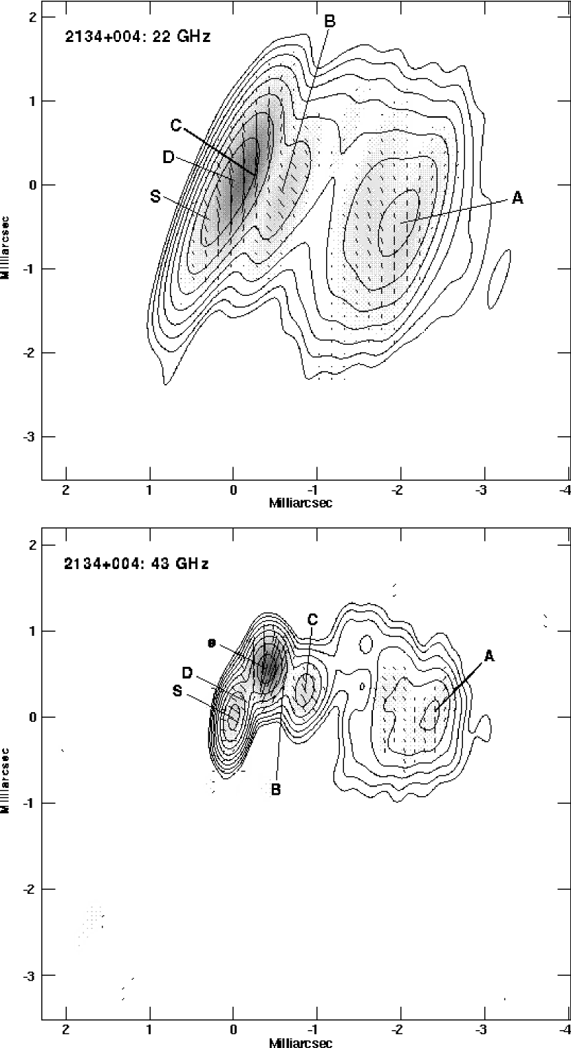
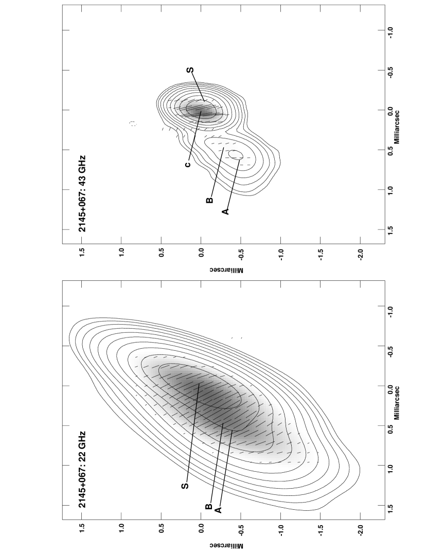
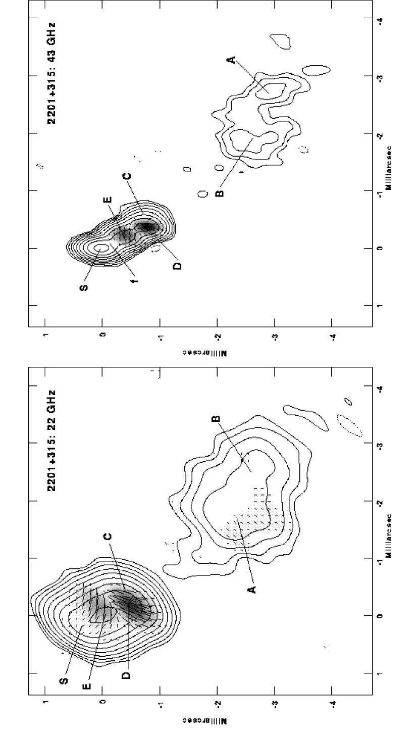
We used the Caltech DIFMAP package (Shepherd et al., 1994) to make Stokes I, Q, and U images of our sources, which we then imported into AIPS to make our final contour images, shown in Figures 1–11. A complete summary of our image parameters is given in Tables 2 and 3. We used a natural visibility weighting scheme for those sources with more diffuse jet structure, as this gives better sensitivity to weak emission.

We performed Gaussian model fits to each source in the uv plane at 22 and 43 GHz using the task “modelfit” in DIFMAP. The results of these fits are given in Tables Intrinsic Differences in the Inner Jets of High- and Low-Optically Polarized Radio Quasars and 5, and are intended as a general guideline for interpreting the polarization structure. Those components that we detected only at 43 GHz (due to the higher angular resolution) are indicated with lowercase letters. We caution that this type of model fitting does not always produce unique results, especially for regions of nearly continuous jet emission. Our procedure was to start with a model composed entirely of CLEAN components, and gradually replace those in the inner few milliarcseconds with Gaussian model components. We added components farther down in the jet in regions where polarized flux was present. While an accurate parameterization of errors is somewhat difficult with this method, we estimate the given positions of strong, isolated components to be accurate to within a quarter of a beam width. For our measured flux densities, we estimate our errors to be $\mathrel{\hbox{\hbox to0.0pt{\hbox{\lower 4.0pt\hbox{$\sim$}}\hss}\hbox{$<$}}}10\%$, in accordance with Gómez et al. (1999) and Mantovani et al. (1999). Our fits are less reliable for very weak components, and those located in regions of diffuse emission.

In Table Intrinsic Differences in the Inner Jets of High- and Low-Optically Polarized Radio Quasars we list the fitted radio core component properties and optical data of our sample sources. We discuss the latter (columns 6, 9, 12, and 15) in §3.3. Columns 2 and 3 give the total core flux density in mJy at 22 and 43 GHz, respectively. We tabulate the core luminosity in column 4, assuming a spectral index $\alpha=0$. Column 5 gives the ratio of core to extended (parsec-scale) flux density at 43 GHz, while columns 7 and 8 indicate the percentage polarization $m$ at the central pixel of the core component at 22 and 43 GHz. The percentage polarization is an indicator of the degree of order in the magnetic field, and is defined as $100\times P/I$, where $P=({Q^{2}+U^{2}})^{1/2}$, and $Q$, $U$, and $I$ are Stokes flux densities. We note that in some cases the peak of polarized emission is offset from that of the $I$ emission, so that the values of $m$ given in Tables Intrinsic Differences in the Inner Jets of High- and Low-Optically Polarized Radio Quasars and 5 may not represent the maximum percentage polarization associated with a particular component. Since all of our polarization detections in Tables Intrinsic Differences in the Inner Jets of High- and Low-Optically Polarized Radio Quasars and 5 are $\mathrel{\hbox{\hbox to0.0pt{\hbox{\lower 4.0pt\hbox{$\sim$}}\hss}\hbox{$>$}}}5\sigma$, we include no corrections for Ricean bias (Wardle & Kronberg, 1974), as these are all negligible. In columns 10 and 11 we list the electric polarization vector position angle $\chi$ for those cores with detected polarized flux at 22 and 43 GHz.

In column 13, we list the ratio of percentage polarization at 43 GHz to that at 22 GHz for those components detected at both frequencies. In order to calculate these values, we matched the uv-coverages as best as possible by flagging visibilities, and using the same restoring beam in the 22 and 43 GHz images. For most sources, it was necessary to shift the re-convolved images so the jet features were coincident at both frequencies. This is due to the self-calibration procedure, which moves the phase reference center to the brightest feature in the image. At 43 GHz, many of the bright cores were resolved into two or more components, which shifted the apparent position of the brightest component by a small, but non-negligible amount. An exact determination of these shifts is difficult, due to the large difference in observing frequencies, and a general lack of steep-spectrum features along the jet with which to register the images. The quantities most affected by registration errors are the spectral index and fractional polarization ratio. The errors in electric vector rotation are not as large, since this quantity does not vary as much from pixel-to-pixel in our images.

We list the measured rotation in $\chi$ between 22 and 43 GHz for the core components in column 14. These values were also obtained using the convolved 43 GHz images. We have applied no overall rotation measure corrections to the data in Tables Intrinsic Differences in the Inner Jets of High- and Low-Optically Polarized Radio Quasars and 5.

In Table 5, we list the same data for the polarized jet components in our sample sources. Columns 2 through 5 give the position with respect to the core, and total flux density of each component at 22 and 43 GHz. Steep-spectrum components that were too faint to be detected at 43 GHz are indicated with a dagger.

Figure 1: VLBA total intensity images of NRAO 140 at 22 and 43 GHz, epoch 1999.03, with electric polarization vectors superimposed. The greyscale in the 22 GHz image indicates linearly polarized intensity ($({Q^{2}+U^{2}})^{1/2}$), where Q and U are the Stokes flux densities.

Figure 2: VLBA total intensity images of 4C 39.25 at 22 and 43 GHz, epoch 1999.03, with electric polarization vectors superimposed. The greyscale indicates linearly polarized intensity.

Figure 3: VLBA total intensity images of 0953+254 at 22 and 43 GHz, epoch 1999.03, with electric polarization vectors superimposed. The greyscale in the 22 GHz image indicates linearly polarized intensity. The position angle of the optical electric vector, epoch 1999.12, is indicated in the 43 GHz panel.

Figure 4: VLBA total intensity images of 3C 273 at 22 and 43 GHz, epoch 1999.03, with electric polarization vectors superimposed. The greyscale indicates linearly polarized intensity . The position angle of the optical electric vector, epoch 1999.12, is indicated in the 43 GHz panel.

Figure 5: VLBA total intensity images of 3C 279 at 22 and 43 GHz, epoch 1999.03, with electric polarization vectors superimposed. The greyscale indicates linearly polarized intensity. The position angle of the optical electric vector, epoch 1999.12, is indicated in the 43 GHz panel.

Figure 6: VLBA total intensity images of 1611+343 at 22 and 43 GHz, epoch 1999.03, with electric polarization vectors superimposed. The greyscale indicates linearly polarized intensity . The position angle of the optical electric vector, epoch 1999.12, is indicated in the 43 GHz panel.

Figure 7: VLBA total intensity images of 1633+382 at 22 and 43 GHz, epoch 1999.03, with electric polarization vectors superimposed. The greyscale in the 22 GHz image indicates linearly polarized intensity. The position angle of the optical electric vector, epoch 1999.12, is indicated in the 43 GHz panel.

Figure 8: VLBA total intensity images of 1928+738 at 22 and 43 GHz, epoch 1999.03, with electric polarization vectors superimposed. The greyscale indicates linearly polarized intensity.

Figure 9: VLBA total intensity images of 2134+004 at 22 and 43 GHz, epoch 1999.03, with electric polarization vectors superimposed. The greyscale indicates linearly polarized intensity.

Figure 10: VLBA total intensity images of 2145+067 at 22 and 43 GHz, epoch 1999.03, with electric polarization vectors superimposed. The greyscale indicates linearly polarized intensity.

Figure 11: VLBA total intensity images of 2201+315 at 22 and 43 GHz, epoch 1999.03, with electric polarization vectors superimposed. The greyscale indicates linearly polarized intensity.

Figure 12: Total optical percentage polarization plotted against that of the unresolved radio core at 43 GHz. The LPRQs are indicated by the open squares, and the HPQs by the filled circles. Upper limits are given for sources with no detected core polarization.

3.3 Optical observations

We obtained optical photopolarimetric data on ten of our sample objects with the Steward Observatory 60-inch telescope at Mt. Lemmon on UT 1999 February 12-14. These were taken with the “Two-Holer” polarimeter/photometer (Sitko, Schmidt, & Stein, 1985), which uses two RCA C31034 GaAs photomultiplier tubes that are sensitive from 3200–8600 Å. Our data acquisition and reduction procedure followed that of Smith et al. (1992). All of our optical observations were unfiltered, and obtained using a $4\arcsec$ circular aperture except for 3C 273, where an $8\arcsec$ aperture and a Kron-Cousins R filter ($\lambda_{c}\sim 6400$ Å) were used. The effective wavelength of the unfiltered observations is $\sim$6000 Å, but is dependent on the shape of the optical spectrum. The fractional degree of linear polarization ($m_{\rm opt}$) listed in Table 4 has been corrected for Ricean bias (Wardle & Kronberg, 1974). In the few instances where only an upper limit can be placed on $m_{\rm opt}$, a 2-sigma limit is listed without any bias correction. In these instances, the polarization position angle, $\chi_{\rm opt}$, is undefined. No correction to these data was made for instrumental polarization since Two-Holer yields $<0.1\%$ polarization for known unpolarized stars. BD+59^∘389 and HD155528 were used to calibrate $\chi_{\rm opt}$ (Schmidt, Elston, & Lupie, 1992).

The observation of 1633+382 on UT 1999 February 14 showed $m_{\rm opt}$ = 7.0$\pm$0.5%. By definition, this measurement places the object into the HPQ category. Previous optical polarimetry never showed this object with $m_{\rm opt}>3$% (Moore & Stockman, 1984; Impey & Tapia, 1990; Impey et al., 1991; Wills et al., 1992a).

The remainder of our sources could not be observed due to observing time and sun-angle constraints; for these we list previously published data from the literature in Table Intrinsic Differences in the Inner Jets of High- and Low-Optically Polarized Radio Quasars. Wherever possible, we used values from Impey & Tapia (1990). These authors attempted to limit observational bias by tabulating only first-epoch polarization measurements for each source made after 1968. For those sources without complete polarization data in Impey & Tapia (1990), we used values from Wills et al. (1992b) and Impey et al. (1991).

Figure 13: Total optical percentage polarization plotted against luminosity of the unresolved radio core component at 43 GHz. The LPRQs are indicated by the open squares, and the HPQs by the filled circles.

Figure 14: Histogram of optical polarization vector ($\chi_{\rm opt}$) offset with respect to the innermost jet direction, with the LPRQs shaded. Values near zero indicate a good alignment between the electric polarization vector and the jet.

4 Results

4.1 Properties of radio core components

One of the main goals of this study is to characterize the magnetic field structures of quasars on the smallest scales, and to look for connections with their optical properties. In this section we discuss new evidence showing that the optical polarization properties of quasars are directly related to those of their unresolved radio core components at 43 GHz.

Figure 15: Histogram of 43 GHz core electric polarization vector offsets with respect to the jet direction, with the LPRQs shaded.

4.1.1 Correlations with optical polarization properties

In Figure 12 we show a log-log plot of core polarization at 43 GHz versus total optical percentage polarization ($m_{\rm opt}$) for our HPQ and LPRQ samples. The relatively small scatter in this plot suggests that these two quantities are related. To evaluate the significance of this correlation (and others presented in this paper), we performed a Kendall’s non-parametric rank test, which uses the relative order of ranks in a dataset to determine the likelihood of a correlation. A test on these variables indicate that this correlation is significant at the 99.995% level.

Previous attempts to find a correlation between radio core and optical polarization have met with only moderate success, due to a lack of sufficient sample size and/or spatial resolution. Impey et al. (1991) found a correlation between total (single-dish) polarization at 15 GHz and optical polarization, which vanished at lower radio frequencies. Since higher radio frequencies sample emission closer to the base of the jet, this strongly argued in favor of the optically polarized emission being emitted close to the core. Gabuzda et al. (1996) found a hint of a possible correlation between 5 GHz radio VLBI core polarization and $m_{\rm opt}$, but had only seven sources in their sample. Cawthorne et al. (1993) observed a larger sample of 24 AGNs from the Pearson-Readhead survey at 5 GHz, but detected VLBI core polarization in only a handful of objects. Recent VLBA observations of these same objects at 43 GHz by Lister et al. (2000) show that some of their non-detections were likely caused by blending of polarized components near the core, which tends to lower the overall degree of polarization. In the case of our sample, 9 of 11 sources had cores at 22 GHz that were in fact a blend of one or more components, as revealed by our 43 GHz data. Indeed, if we compare optical polarization with total integrated polarization at 43 GHz for our objects, the correlation significance drops to 83%.

We find the level of optical polarization to be positively correlated with several other source properties at the 95% level or higher. These are 43 GHz core luminosity, total spectral index between 43 and 22 GHz, and core dominance ($R$). The latter quantity is defined as the ratio of core to extended (parsec-scale) flux at 43 GHz. Impey & Tapia (1990) found a similar correlation between $m_{\rm opt}$ and $R$ for the Kühr 2 Jy sample of radio sources but found no correlation between $R$ and total integrated polarization at 5 GHz. We obtain a similar null result for $R$ and total polarization level at 43 GHz, but find that $R$ is positively correlated with the core polarization level at the 99.6% confidence level.

These correlations all indicate that the more optically polarized quasars have brighter radio cores at 43 GHz, as a bright core tends to flatten the spectral index and increase $R$. We plot optical polarization versus 43 GHz core luminosity for our samples in Figure 13.

4.1.2 Electric vector position angles

Despite the strong correlation between optical and 43 GHz core polarization, we find no correlation between the electric vector position angles ($\chi$) at these two wavelengths (observed approximately a month apart) for the entire dataset. A similar null result was found at lower radio frequencies by Rusk & Seaquist (1985) in their analysis of a larger sample of radio-loud quasars. It is unlikely that the electric vectors are significantly affected by Faraday rotation at 43 GHz, given the typical nuclear rotation measures of quasars seen in this sample and others ($\mathrel{\hbox{\hbox to0.0pt{\hbox{\lower 4.0pt\hbox{$\sim$}}\hss}\hbox{$<$}}}3000\;\rm\ rad\ m^{-2}$; see §5). A more likely explanation is that the polarization vectors have rotated in the time interval between the optical and radio measurements. This would imply that the $\chi$’s of blazars are significantly more variable than their fractional polarizations. Indeed, rapid swings in $\chi$ are not uncommon in blazars (e.g., Aller et al., 1999), with changes sometimes occurring on timescales $\mathrel{\hbox{\hbox to0.0pt{\hbox{\lower 4.0pt\hbox{$\sim$}}\hss}\hbox{$<$}}}2$ weeks (Gabuzda et al., 1998). Another possibility is that the optically polarized emission may be originating in a strongly shocked component in the jet, instead of the core. Gabuzda et al. (1996) found evidence for this in a small sample of BL Lacertae objects observed at 5 GHz.

If we restrict our analysis to those sources in our sample with near-simultaneous optical and radio observations, we find similar alignments of $\chi_{\rm opt}$ with those of jet components in four of five sources (3C 279, 3C273, 1611+343, and 0953+254) at 43 GHz. The only source with similar 43 GHz core component $\chi$ and $\chi_{\rm opt}$ is 1611+343. Due to the large range of $\chi$ seen in the jets of some sources and the small number of sources, it is possible that these alignments are merely due to chance. A proper study of radio/optical $\chi$ alignments requires truly simultaneous optical and radio observations over a sufficient timescale to determine whether changes in the optical $\chi$’s follow those seen in the radio jets, or the unresolved core components.

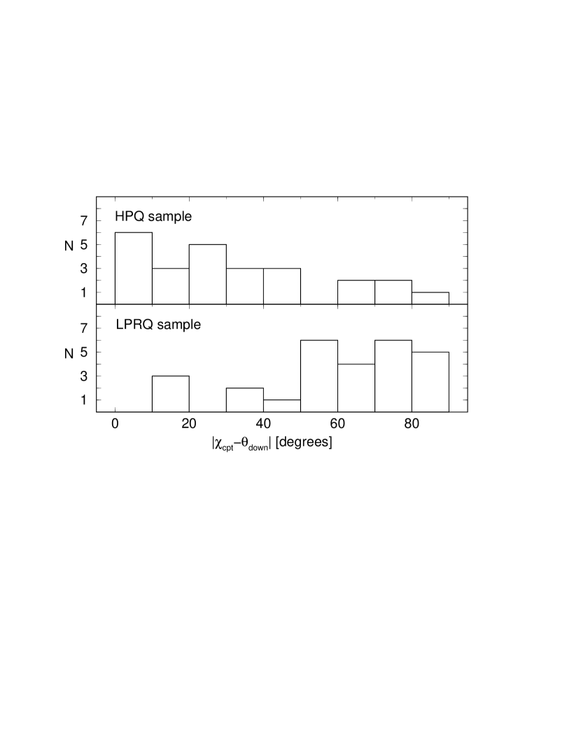
Many previous VLBI polarization studies have compared the optical and radio $\chi$’s to the jet direction near the core ($\theta_{jet}$), as the simplest form of the shock-in-jet model predicts that a strong transverse shock will preferentially strengthen the perpendicular component of an initially tangled magnetic field. In the absence of any Faraday rotation, the electric vectors of the shocked region will be rendered parallel to the jet. In Figure 14 we plot the distribution of $|\chi_{\rm opt}-\theta_{jet}|$ for our samples. This quantity represents the difference between the optical $\chi$ and the direction of the jet closest to the core. We define $\theta_{jet}$ as the position angle of the innermost jet component with respect to the core. Due to the $180\arcdeg$ ambiguity in the measured polarization position angles, $|\chi_{\rm opt}-\theta_{jet}|$ can never exceed $90\arcdeg$. The overall distribution is peaked at zero, where the optical $\chi$’s are parallel to the jet. This is in agreement with the results of previous studies (Impey, 1987; Rusk, 1990; Impey et al., 1991). The distribution for the LPRQs (shaded) is possibly bi-modal, with peaks at zero and roughly 60°, which was also seen by Impey et al. (1991) in a much larger sample.

We plot an analogous distribution for the radio core $\chi$’s at 43 GHz in Figure 15. Only four LPRQ cores are shown in this plot, since the remainder did not have any detectable polarized flux at 43 GHz. Again the distribution is peaked near zero, and only two sources have core magnetic fields that are roughly parallel to the jet ($|\chi_{\rm opt}-\theta_{jet}|\mathrel{\hbox{\hbox to0.0pt{\hbox{\lower 4.0pt\hbox{$\sim$}}\hss}\hbox{$>$}}}70\arcdeg$). We find that all of the highly polarized cores with $m_{43}>3\%$ have core $\chi$’s aligned to within $30\arcdeg$ of the local jet direction. These findings support the scenario described in §4.1.1, in which the core polarization in these sources originates in a shock near the base of the jet.

Figure 16: Percentage polarization of jet components at 43 GHz plotted against projected distance from the core in parsecs.

4.2 Jet properties

The steep radio spectral indices of AGN jets ($\alpha\sim-0.8$) generally cause them to drop below the sensitivity level of current high-frequency VLBI images at distances of more than a few milliarcseconds from the core. Nevertheless, the large improvement in angular resolution and reduced source opacity at high frequencies allow for a more thorough investigation of the nature of AGN jets close to the core. In this section we discuss the overall jet polarization properties of our combined HPQ and LPRQ samples.

The strongest trend we find in the inner jets of our sample is an steady increase in fractional polarization as you move downstream from the core. There is no significant decrease in total intensity with core distance, however, as was seen in the sample of Cawthorne et al. (1993) at 5 GHz, which covered regions farther down the jet ($\sim 10-90$ pc, projected). Figure 16 shows an increase in $m_{43}$ with distance down the jet, for both LPRQs and HPQs. A similar trend exists in the 22 GHz data. A Kendall’s tau test shows these variables are correlated at a significance level of $\sim 99.99\%$. This increase in polarization with distance was also seen in quasars (but not in BL Lac objects) at 5 GHz by Cawthorne et al. (1993), who attributed it to interaction of the jet boundary with the external medium. According to these authors, the jet material experiences shear as it moves down the jet, which organizes its (initially random) magnetic field, and increases the degree of polarization. We note that the limited dynamic range of our images does not allow us to measure the polarization of the underlying jet in most sources, however, but rather that of polarized knots associated with shocks.

Figure 17: Top panel: electric polarization vector offset with respect to the local downstream jet direction plotted against fractional polarization, for polarized jet components. Bottom panel: same plot for upstream jet directions.

Figure 18: Top panel: electric polarization vector offset with respect to the local downtream jet direction plotted against projected distance from the core in parsecs. Bottom panel: same plot for upstream jet directions.

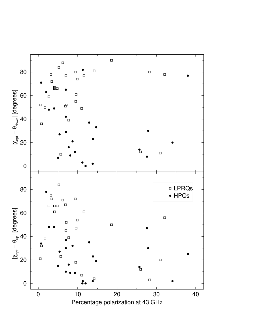
We performed a similar analysis to §4.1.2 by comparing the $\chi$ of each polarized component to the local jet direction. Because many of the jets in our sample undergo significant bends, the latter quantity is ambiguous in some cases. We therefore list two local jet directions for each component in Table 5: $\theta_{\rm up}$ represents the direction of the jet ridgeline upstream of the component, and $\theta_{\rm down}$ represents the jet direction downstream. In cases where nearby jet emission was weak or absent, we used the position of the nearest upstream and downstream components to establish the local jet direction.

We find an anticorrelation (Kendall’s tau = $-0.315$; 99.9% significance) between fractional polarization and $|\chi_{\rm cpt}-\theta_{\rm up}|$ (lower panel of Fig. 17), where $\chi_{\rm cpt}$ is the electric vector position angle of the component at 43 GHz. There is a loosely defined upper envelope to this distribution, such that there are no highly polarized components with magnetic fields parallel to the jet. We find no significant correlation (Kendall’s tau = $-0.117$; 78.3% significance) using the downstream position angles, plotted in the top panel of Fig. 17.

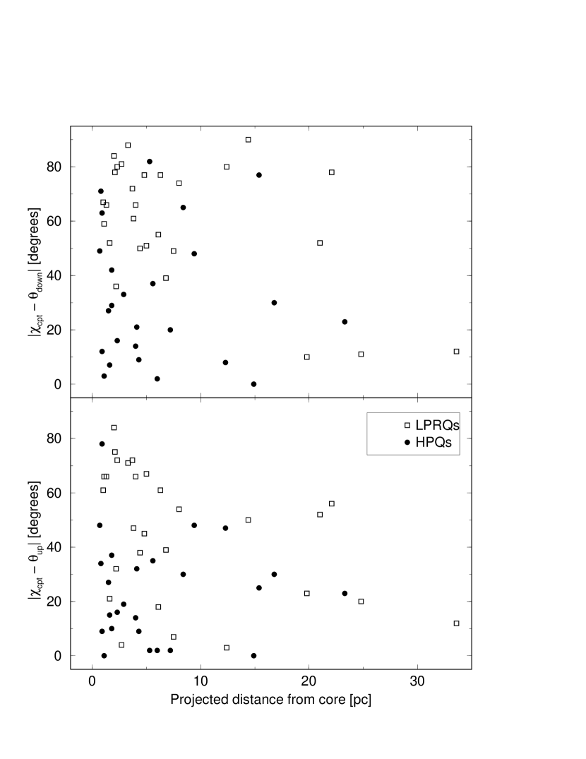
We also find an upper envelope in the plot of $|\chi_{\rm cpt}-\theta_{\rm up}|$ versus projected core distance (lower panel of Fig. 18). All of the components with magnetic fields nearly parallel to the jet are located very close to the core. Furthermore, these components are all associated with LPRQs (with the exception of component c2 of 1633+382, a quasar that would have been classified as an LPRQ prior to our optical observation on UT 1999 February 14).

The increasing longitudinal field model of Cawthorne et al. (1993) has difficulty accounting for the trends in Figs. 17 and 18. If we assume that the viewing angle and shock strengths are constant along the jet, the $\chi$’s should become more perpendicular to the jet with increasing distance from the core. This is the opposite of what is seen. Also, this model predicts that the fractional polarization of components with $\chi$’s parallel to the jet should not be appreciably lower than those with perpendicular orientations, which is not the case. For these reasons, we do not believe the trend of increasing fractional polarization with distance is caused by an underlying longitudinal magnetic field of increasing strength. More likely, this trend is due to either an increase in shock strength with distance, or jet curvature. Although shock strengths are generally difficult to estimate without good determinations of shock speed and jet orientation, a test of the curvature scenario may be relatively straightforward.

Figure 19: Distribution of polarization vector rotation between 22 and 43 GHz for polarized jet components.

Given the high luminosities of the core components of our sample, it is likely that they are associated with the most highly aligned portions of the jet, and are seen at very small viewing angles. If the jets have simple monotonic bends, they will then be curving away from the line of sight. This appears to be the case for the gamma-ray blazars detected by EGRET (Marchenko et al., 2000). According to the simple transverse shock model (Hughes et al., 1985), the polarization of a bent jet should increase along the jet as the viewing angle increases from originally small values, due to aberration. Even if the bends are not monotonic, the projected core distance will not increase very rapidly in those portions of the jet which are bending toward us, thereby preserving the trend seen in Fig. 16. This bending model could be tested, for example, by simultaneously measuring the inter-knot polarization levels and superluminal speeds along the jet, as these are both affected by orientation in a predictable manner. We will return to the role of orientation and shock strength in our discussion of HPQ and LPRQ properties in §6.

Figure 20: Ratio of percentage polarization at 43 and 22 GHz for jet components plotted against the spatial resolution of the restoring beam.

Figure 21: Plots of various source quantities against jet misalignment between parsec and kiloparsec scales. In top panel is the ratio of core to extended flux at 43 GHz, the middle panel shows optical percentage polarization, and the lower panel shows integrated spectral index between 22 and 43 GHz.

5 Comparison of magnetic field properties at 22 and 43 GHz

Based on the typical integrated rotation measures of AGNs at cm-wavelengths ($\mathrel{\hbox{\hbox to0.0pt{\hbox{\lower 4.0pt\hbox{$\sim$}}\hss}\hbox{$<$}}}200$ $\ \rm rad\ m^{-2}$: Wrobel 1993; O’Dea 1989), we would expect to see very few differences in the polarization properties of our sample at 22 and 43 GHz, with the exception of some spatial resolution effects. Recent VLBI polarization studies (e.g. Taylor, 1998; Udomprasert et al., 1997) have shown, however, that on parsec-scales the measured rotation measures are generally much higher ($>1000$ $\ \rm rad\ m^{-2}$). The most likely origin of these high RMs is external Faraday rotation by gas in the narrow-line region (Taylor, 1998). In this section we discuss the evidence for strong depolarization and Faraday rotation effects in our LPRQ sample.

5.1 Core components

In columns (13) and (14) of Table Intrinsic Differences in the Inner Jets of High- and Low-Optically Polarized Radio Quasars we list the rotation in $\chi$ and ratio of percentage polarization at 43 GHz to that at 22 GHz for the core components in our sample. Since several of the cores had no detectable polarization at 43 GHz, we tabulate data for six cores only. The depolarization ratios lie between 0.5 and 2.3, while the $\chi$’s are rotated between 2 and 19 degrees. If we assume that these $\chi$’s at 22 and 43 GHz follow a standard $\lambda^{2}$ law, we can convert the latter into rest-frame rotation measures using $RM_{rest}=130.19\;\Delta\chi(1+z)^{2}\ \rm rad\ m^{-2}$, where $\Delta\chi$ is the $\chi$ shift in degrees. Given the uncertainty in our absolute $\chi$ correction ($\mathrel{\hbox{\hbox to0.0pt{\hbox{\lower 4.0pt\hbox{$\sim$}}\hss}\hbox{$<$}}}5^{o}$), this yields rotation measures between 0 and $\sim 6000\ \rm rad\ m^{-2}$, which are consistent with values found by Taylor (1998) for core-dominated quasars.

We find a tendency for sources with flatter total (i.e., single dish) spectral indices between 1.4 and 5 GHz to have smaller $m_{43/22}$ ratios (99.5% confidence according to Kendall’s tau). Since the total spectral index tends to be steeper for sources with weaker cores, this may indicate the presence of both Faraday and opacity effects in the core region at longer wavelengths. This opacity makes it difficult to interpret trends involving the $m_{43/22}$ ratio, as we may simply be sampling spatially distinct regions of different intrinsic polarization at these two wavelengths. Observations at an intermediate frequency are required to investigate this in more detail.

5.2 Jet components

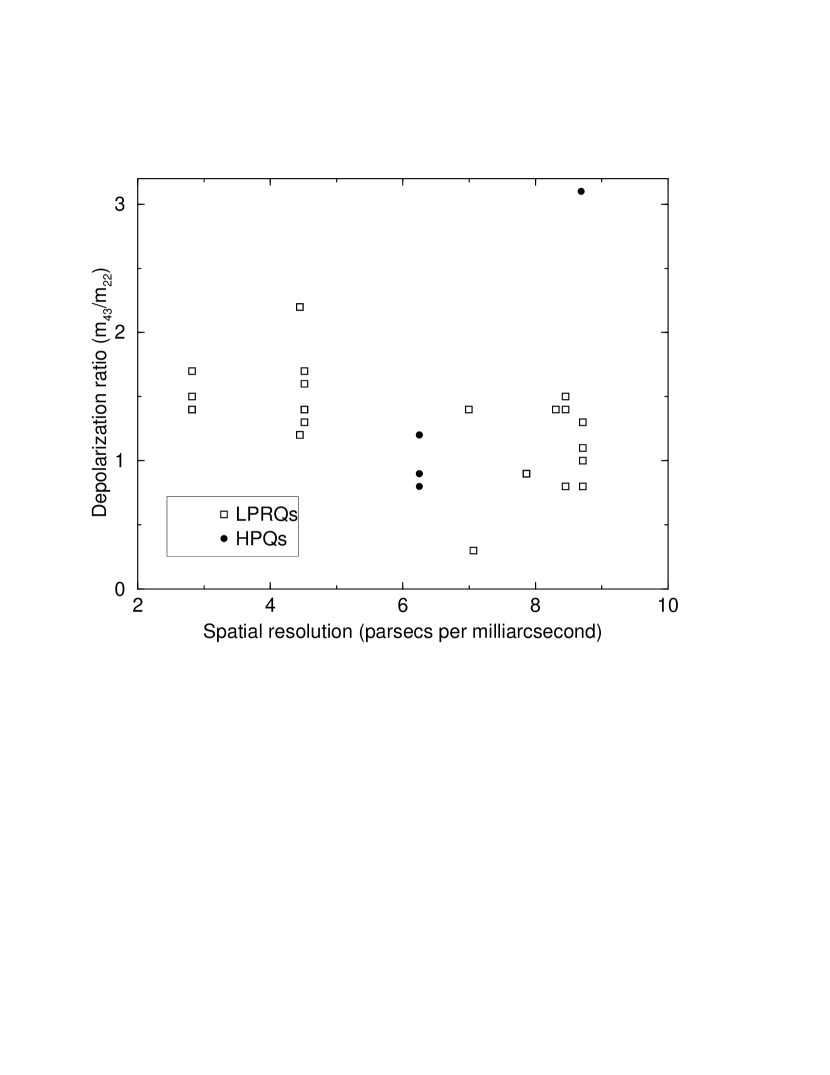
In Figure 19 we show the distribution of $\Delta\chi=|\chi_{43}-\chi_{22}|$ for the polarized jet components in our AGN sample. Although the majority have $\Delta\chi<15^{o}$, there are three with substantial $\chi$ rotations. These components are all very weakly polarized ($<1\%$) at 22 GHz.

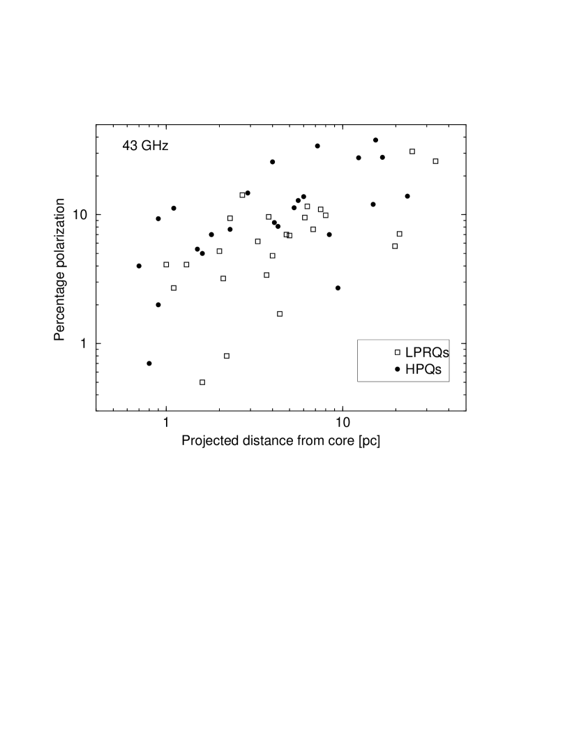
The fractional polarization ratios generally lie between 0.8 and 1.8, with a median value of $\sim 1.2$. We find these ratios are related to the spatial resolution of our images, with the low-redshift sources displaying significantly higher values (Fig. 20). Tribble (1991) has shown that polarization fluctuations can occur in uniform (non-clumpy) external Faraday screens, due to turbulent magnetic fields. It is possible that in higher-redshift sources in our sample, these fluctuations are being smeared out by the larger spatial extent of the beam, leading to lower average depolarization factors. This effect needs to be investigated further using larger samples, as multi-frequency polarimetry is potentially a very useful tool for probing the material in the central regions of AGNs.

6 Observed differences between high- and low-optically polarized quasars

Various claims have been made in the literature that the differences in high- and low-optically polarized radio quasars are due to their jets having different viewing angles, with LPRQs lying farther away from the line of sight. Supporting evidence for this scenario includes differences in their variability timescales (Valtaoja et al., 1992), and their distributions of jet misalignments between parsec and kiloparsec scales (Impey et al., 1991; Xu et al., 1994). In this section we examine this hypothesis, and show that it cannot fully account for differences seen in the parsec-scale magnetic fields of LPRQs and HPQs.

6.1 Core properties

In section 4.1.1 we showed that the level of optical polarization in compact quasars is closely related to that of the radio core at 43 GHz. The correlation in Fig. 12 suggests that the optically polarized and radio emission arise from the same process, (i.e., synchrotron radiation), and may in fact be co-spatial. They must also be beamed by a similar amount, since any difference in Doppler factor would change the observed fractional polarization (due to aberration) and destroy the correlation. A likely scenario, presented in previous studies (e.g., Gabuzda et al., 1996), is that both the radio and optically-polarized flux arise from a single energy distribution of electrons, located very close to the base of the jet. The rapid variability and high degrees of optical polarization seen in most blazars imply that the polarized emission arises in a very small region having a well-ordered magnetic field. These conditions are most readily created in a relativistic shock, in which the level of observed polarization depends on both the shock strength and viewing angle in the source frame (e.g., Hughes et al., 1985).

The continuous trend in Figure 12 suggests that the division between HPQs and LPRQs at $m_{\rm opt}=3\%$ may be an arbitrary one in the case of compact radio quasars. Nevertheless, we will retain this classification criterion for the purposes of comparing the general properties of high- and low-polarization quasars in this paper.

We have performed Kolmogorov-Smirnov tests on various properties of our HPQ and LPRQ samples to determine the probability that they are drawn from the same population. We list the results of these tests in Table 6. The cores of our LPRQ sample in our sample are fainter on average, and are more weakly polarized than those of the HPQs. As a result, the LPRQs are less core-dominated, and have steeper total spectral indices between 22 and 43 GHz. Although it appears that the core magnetic fields of HPQs favor perpendicular orientations with respect to the jet (see Fig. 15), there are insufficient data to characterize those of the LPRQs.

Figure 22: Distribution of 43 GHz electric polarization vector misalignment of polarized jet components with respect to the local upstream jet direction ($\theta_{\rm up}$) for HPQs (top) and LPRQs (bottom).

Figure 23: Same as Fig. 22, using the local downstream jet direction $\theta_{\rm down}$.

6.2 Jet Bending

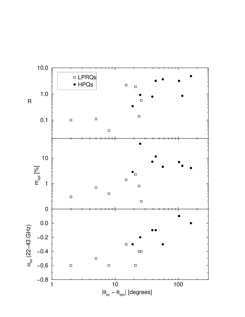
Many bright, compact radio quasars are known to exhibit large apparent bends in their jets that are likely exaggerated by projection effects associated with small angles to the line of sight. The amount of apparent jet bending in a sample of objects should therefore be statistically related to the mean viewing angle. Previous bending studies (e.g. Tingay, Murphy, & Edwards, 1998) have used two main statistics to quantify the amount of bending: $\phi_{T}$, which represents the total amount of bending along the jet (in degrees), and $\Delta\theta$, which is defined as the difference in the innermost jet position angle on parsec and kiloparsec scales. Neither of these parameters is wholly satisfactory, since they may be influenced by the spatial resolution and dynamic range of the radio images used to calculate them. In order to lessen the effects of the latter, in this paper we measure $\phi_{T}$ out to 15 (projected) parsecs along the jet. We use the best images available in the literature to measure the jet position angles on kiloparsec scales. We list these data in Table Intrinsic Differences in the Inner Jets of High- and Low-Optically Polarized Radio Quasars.

Despite the potential shortcomings of these bending parameters, we find them to be correlated with several other source properties. The more misaligned jets in our sample tend to have larger core-to-extended flux ratios at 43 GHz, and flatter integrated 22/43 GHz spectral indices. They are also more polarized in the optical regime (Fig. 21). A KS test shows that the misalignment distributions of our LPRQs and HPQs differ at the 98.7% confidence level. A similar result was found by Impey et al. (1991) for the Pearson-Readhead sample, and Xu et al. (1994) for the much larger Caltech-Jodrell survey.

To first order, these trends are easily explained by the orientation model: HPQs, having smaller viewing angles, should have larger apparent pc-kpc jet misalignments, and more highly beamed cores. This will also increase their core-to-extended flux ratios, and flatten their overall spectral indices. In the optical, the polarized flux from the core would be boosted with respect to the continuum from the accretion disk, which would raise the overall level of polarization. Upon deeper inspection, however, this model displays several shortcomings. If the polarized flux in the core arises from one or more planar shocks, the inner jets of LPRQs, lying farther away from the line of sight than the HPQs, should have higher fractional polarizations, according to the standard shock model of Hughes et al. (1985). This is the opposite of what is observed. We also find no differences in the total amount of bending out to 15 pc in LPRQs and HPQs, which is difficult to reconcile with the orientation hypothesis. Finally, there are two trends with $\phi_{T}$ that are present only in the LPRQ data: the amount of total jet bending increases with core luminosity and optical polarization level.

6.3 Jet properties

In addition to having different core properties, HPQs and LPRQs show fundamental differences in their parsec-scale jets. First, the median jet component luminosity of the LPRQs (26.2 W/Hz) is marginally lower than the HPQs (26.7 W/Hz), and second, the polarized components in HPQ jets tend to have magnetic fields that are perpendicular to the jet (Figs. 22 and 23). Those of LPRQs have a tendency to be more parallel to the jet, although this depends somewhat on whether we compare the $\chi$’s to the upstream or downstream jet direction. The percentage polarizations of the jet components are similar for the two classes (Fig. 24).

These last two findings effectively rule out the possibility that the differences between LPRQs and HPQs are due to orientation alone. If LPRQ and HPQ jets are intrinsically identical, and seen at different viewing angles, we expect to see large differences in observed fractional polarization, since this quantity varies as $\cos^{2}{\epsilon}/(A-\cos^{2}{\epsilon})$, where ${\epsilon}$ is the angle between the plane of the shock and the line of sight in the rest frame of the emitting gas, and $A$ is a function of shock strength (Hughes et al., 1985).

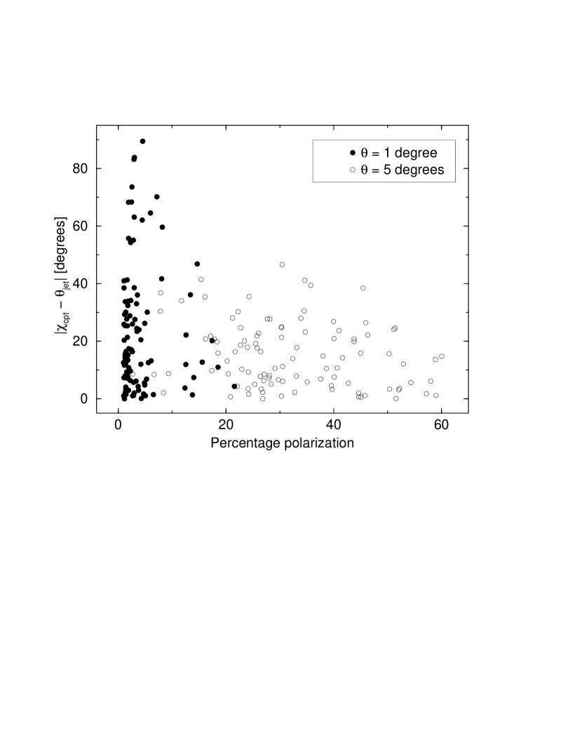
It is also not possible to transform the observed $|\chi_{\rm cpt}-\theta_{jet}|$ distribution for HPQs into that of the LPRQs simply by changing the jet orientation. Indeed, in the case of strong transverse shocks, the observed electric vectors will remain parallel to the jet, independent of viewing angle (Blandford & Königl, 1979). To produce a change in $\chi$ with orientation it is necessary to invoke either an underlying longitudinal magnetic field (e.g., Kollgaard et al., 1990), or oblique shocks. We have used the model of Lister et al. (1998) to calculate the observed $\chi$’s and percentage polarizations of a population of moving, oblique shocks at two different viewing angles. These shocks move at a variety of speeds down a jet whose underlying flow has a bulk Lorentz factor of 15. In Figure 25 we show a plot of $|\chi-\theta|$ vs. percentage polarization for the same family of shocks, seen at 1 degree from the line of sight (filled circles) and 5 degrees (open circles). As the viewing angle is increased, the components become more polarized, and their $\chi$’s become more aligned with the jet. This behavior is inconsistent with a model in which LPRQs have larger viewing angles than their HPQ counterparts.

Figure 24: Distribution of percentage polarization for jet components in HPQs (top) and LPRQs (bottom).

6.4 Discussion

Many of the properties of HPQs and LPRQs that we have discussed in this paper appear difficult to reconcile using a single model. While the bending properties and core luminosities suggest possible differences in viewing angle and Doppler factor, the jet polarization properties suggest otherwise. In this section we discuss possible ways in which to reconcile these seemingly contradictory findings.

Figure 25: Simulated electric polarization offset with respect to local jet direction, plotted against fractional polarization for a population of moving, oblique shocks. The filled circles represent a viewing angle of 1 degree to the jet, while the empty circles represent the same jet viewed at 5 degrees from the line of sight.

6.4.1 Shock strengths

The simplest way to account for the jet polarization properties of LPRQs is to assume that their shocks are weaker than those of HPQs, and increase in strength with distance from the core. Their underlying jet magnetic field cannot be randomly oriented, but must be somewhat longitudinal to account for the $\chi$ orientations near the core. This scenario can explain the lower core polarizations and luminosities in LPRQs, and reproduces the trends of polarization and $\chi$ alignment with distance down the jet. The differences in shock strengths may also be responsible for the different optical $\chi$ misalignment distributions of LPRQs and HPQs reported by Impey et al. (1991). A recent high-resolution optical and radio study of M87’s jet by Perlman et al. (1999) showed that the optically polarized emission in the inner jet comes primarily from bright, shocked regions with magnetic fields perpendicular to the jet. Strong shocks are apparently required to boost and maintain the electron energies at levels where they are able to emit optical synchrotron radiation.

It is also possible to incorporate this shock strength model into the evolutionary scheme of Fugmann (1988), who found that at any given epoch, only $\sim 2/3$ of flat-spectrum quasars show blazar-like properties. If the LPRQs in our sample are in a temporary quiescent state, the more polarized shocks located down the jet may be relics from previous “blazar” epochs when the source was emitting more strongly-shocked components. We would also expect to see LPRQs that have recently transformed into HPQs by emitting shocked components: the former LPRQ 1633+382 may be an example of such an object. Our images reveal a highly polarized component near the core that may have triggered its dramatic increase in optical polarization. The “duty cycle” (the fraction of time that $m_{\rm opt}$ is $>3\%$) of LPRQs is still not well determined, however, as there have been no systematic, long-term polarimetric monitoring studies of these objects. Polarization variability is likely to be a better indicator of blazar activity than the traditional $m_{\rm opt}>3\%$ criterion, since the latter can be affected by the strength of the non-synchrotron optical continuum.

6.4.2 Jet orientation

Although we cannot completely rule out possible differences in the orientation of HPQ and LPRQ jets, we consider it unlikely that they differ by a large amount. Any change in viewing angle would have to be offset by a complimentary change in shock or longitudinal field strength, or alternatively, jet speed, in order to reproduce the similar radio component polarization levels seen in both classes. The similarities in redshift, emission-line equivalent width, and optical luminosities of HPQs and LPRQs (Moore & Stockman, 1984; Wills et al., 1992a) suggest that they undergo similar amounts of relativistic beaming. Also, Murphy et al. (1993) find no differences in their core-to-extended flux ratios, which should be a good indicator of beaming (e.g., Antonucci & Ulvestad, 1985).

One possibility is that the observed differences in the parsec/kiloparsec-scale jet misalignment angle could simply be due to a higher degree of intrinsic bending in HPQs, and not orientation. However, given the similarities in the $\phi_{T}$ distributions, this does not seem likely. Alternatively, the LPRQs may represent jets whose bends lie in a plane perpendicular to that of the sky. Monte Carlo simulations of bent jet populations (Lister, 1999) have shown that flux-limited samples should contain a certain fraction of these AGNs, whose innermost jets start out with moderately high viewing angles, but then bend into the line of sight. In these cases, the highly-aligned portion of the jet would likely obscure any upstream emission, and might be mistakenly identified as the core due to its large Doppler factor. The parsec-scale jets of these sources would have the same small viewing angles as typical HPQs, but would fade out faster with core distance, and be much better aligned with their kiloparsec-scale structure. We are currently gathering 43 GHz VLBI polarimetry and space-VLBI data on a large, complete sample of LPRQs and HPQs (the Pearson-Readhead survey; Pearson & Readhead 1988) with which we will be able to investigate these scenarios more fully.

7 Conclusions

In this paper we have used high-frequency VLBI and optical polarimetry to compare the parsec-scale magnetic field properties of a sample of high-optical polarization, compact radio quasars with a sample of similar objects having low optical polarizations. We summarize our results as follows:

1. We find a strong correlation between the level of optical polarization and radio core polarization at 43 GHz. The more optically polarized quasars also have higher core luminosities, core-to-extended flux ratios, and flatter integrated 22/43 GHz spectral indices. These trends strongly indicate that the optically polarized emission is synchrotron radiation, and is co-spatial with the radio core emission at 43 GHz.

2. The electric vectors of the highly polarized 43 GHz radio cores are roughly aligned with the inner jet, indicating magnetic fields perpendicular to the flow. A similar configuration is seen in the optical, suggesting that the polarized flux at both wavelengths is due to one or more strong transverse shocks located very close to the base of the jet.

3. There is a strong trend for the fractional polarizations of bright jet components to increase downstream from the core. The fact that all of the components with magnetic fields parallel to the jet are located near the core suggests that this trend is not due to an underlying longitudinal magnetic field of increasing strength. Rather, we believe it is either the result of the jet curving away from the line of sight, or an increase in shock strength along the jet.

4. We find evidence for large rotation measures (up to $\sim 3000\ \rm rad\ m^{-2}$) in the nuclear regions of low-optically polarized radio quasars, which are indicative of parsec-scale Faraday screens with organized magnetic fields. The low-redshift quasars in our sample tend to have jet components with larger 43/22 GHz depolarization ratios than those found in the high-redshift sources. This might be due to small-scale magnetic field fluctuations in the Faraday screens that are being smeared out in the high-redshift sources by the poorer spatial resolution of the restoring beam.

5. We find that the parsec-scale jet properties of compact radio quasars are highly dependent on their level of optical polarization. Sources with optical fractional polarizations below $3\%$ (low-optically polarized radio quasars: LPRQs) tend to have lower 43 GHz core polarizations, fainter cores, steeper total spectral indices, smaller pc/kpc-scale jet misalignments, and smaller core-to-extended flux ratios than high-optically polarized quasars (HPQs). Although the components in the jets of HPQs and LPRQs have similar fractional polarizations, those found in HPQs tend to have magnetic fields that are perpendicular to the jet, while those in LPRQ jets have mainly parallel orientations.

6. The observed differences in LPRQs and HPQs cannot be fully explained by a model in which LPRQs are seen at larger angles from the line of sight. Instead, our data are more consistent with an evolutionary scenario based on Fugmann (1988), in which flat-spectrum quasars go through episodic stages of blazar-like activity. During these phases, they emit strongly shocked components with transverse magnetic fields, which move at a variety of speeds down the jet. LPRQs may represent quiescent phases of blazars in which only weak shocks are generated in the flow.

Table 1: Overall Radio Source Properties

Source	Epoch	z	$\alpha$	$L_{22}$	$L_{43}$	$m_{43}$	$\theta_{kpc}$	$\theta_{pc}$	$\phi_{tot}$	Ref.
[1]	[2]	[3]	[4]	[5]	[6]	[7]	[8]	[9]	[10]	[11]
Low polarization quasars
NRAO 140	1999 Jan 12	1.258	$-0.36$	27.84	27.71	0.8	143	138	28	1
4C 39.25	1999 Jan 12	0.695	0.82	28.10	27.93	7.1	76	68	40	2
0953+254	1999 Jan 12	0.712	0.43	27.15	27.07	11.9	$-109$	$-124$	68	1
3C 273	1999 Jan 12	0.158	$-0.11$	27.40	27.24	6.6	$-130$	$-128$	15	3
1611+343	1999 Jan 12	1.401	$-0.12$	28.27	28.11	9.0	$-170$	169	170	1
1928+738	1999 Jan 12	0.302	$-0.07$	26.87	26.74	2.8	$-170$	166	177	4
2134+004	1999 Jan 12	1.932	0.83	28.74	28.59	7.4	$\cdots$	$-29$	87	$\cdots$
2145+067	1999 Jan 12	0.990	0.29	28.38	28.38	4.4	$\cdots$	72	70	$\cdots$
2201+315	1999 Jan 12	0.295	0.20	26.82	26.70	3.7	$-127$	$-153$	14	1
High polarization quasars
0420–014	1998 Jul 31	0.915	0.67	27.96	27.88	1.7	171	$-132$	55	6
1055+018	1996 Nov 23	0.888	0.22	$\cdots$	27.83	9.0	$-179$	$-63$	20	1
3C 279	1999 Jan 12	0.536	0.02	28.31	28.26	11.5	$-153$	$-128$	27	5
1334–127	1996 Nov 23	0.539	0.13	$\cdots$	27.90	5.2	$\cdots$	139	12	$\cdots$
1510–089	1998 Jul 31	0.360	$-0.01$	26.74	26.75	4.0	163	$-38$	57	7
1633+382	1999 Jan 12	1.814	0.42	28.27	28.29	7.0	176	$-81$	136	1
3C 345	1998 Jul 31	0.593	0.05	27.89	27.86	5.3	$-32$	$-76$	163	8
CTA 102	1998 Jul 31	1.037	$-0.46$	28.18	28.15	4.3	147	108	41	6
3C 454.3	1998 Jul 31	0.859	0.11	28.31	28.23	6.4	$-61$	$-80$	35	1

Note. — Luminosities are calculated assuming $H_{o}=65\ \rm km\ s^{-1}\ Mpc^{-1}$, $\Lambda=0$, and $q_{o}=0.1$. Columns are as follows: (1) Source name. (2) UT date of VLBA radio observations. (3) Redshift. (4) Spectral index between 1.4 and 5 GHz, obtained from NED. (5) Total luminosity at 22 GHz in $\rm W\ Hz^{-1}$, from Metsähovi single dish data. (6) Parsec-scale luminosity at 43 GHz in $\rm W\ Hz^{-1}$, derived from cleaned flux in VLBA maps. (7) Parsec-scale integrated percentage polarization at 43 GHz. (8) Innermost jet position angle on kiloparsec scale. (9) Innermost jet position angle on parsec scale. (10) Total amount of bending along jet (in degrees) out to a projected distance of 15 pc from the core. (11) Reference for image used to measure values in columns 8 and 10.

References. — (1) Murphy et al. 1993; (2) Marscher et al. 1991; (3) Davis, Muxlow, & Conway 1985; (4) Kollgaard, Wardle, & Roberts 1990; (5) de Pater & Perley 1983; (6) Antonucci & Ulvestad 1985; (7) Price et al. 1993; (8) Kollgaard, Wardle, & Roberts 1989.

Table 2: Summary of 22 GHz VLBA image parameters

Source	Type	Weight	Beam	PA	Flux	EV	RMS	DNR	Peak	Contour levels
[1]	[2]	[3]	[4]	[5]	[6]	[7]	[8]	[9]	[10]	[11]
NRAO 140	IPOL	Natural	0.85 x 0.43	$-20$	1.594		0.4	3559	1238	$-0.1$, 0.1, 0.2, 0.4, 0.8, 1.6, 3.2, 6.4, 12.8, 95
	PPOL				0.029	17	0.3	24	7.1
4C 39.25	IPOL	Uniform	0.60 x 0.35	$-10$	10.415		2.0	2525	5150	$-0.15$, 0.15, 0.3, 0.6, 1.2, 2.4, 4.8, 9.6, 19.2, 38.4, 76.8
	PPOL				0.374	267	1.2	180	215
0953+254	IPOL	Uniform	0.83 x 0.35	$-22$	1.078		0.8	818	648	$-0.3$, 0.3, 0.6, 1.2, 2.4, 4.8, 9.6, 19.2, 38.4, 76.8
	PPOL				0.038	100	0.6	26	15.6
3C 273	IPOL	Uniform	0.97 x 0.38	$-16$	35.237		6.1	2820	17256	$-0.15$, 0.15, 0.3, 0.6, 1.2, 2.4, 4.8, 9.6, 19.2, 38.4, 76.8
	PPOL				1.699	400	3.4	217	738
3C 279	IPOL	Uniform	0.99 x 0.35	$-11$	27.649		3.6	4108	14789	$-0.1$, 0.1, 0.2, 0.4, 0.8, 1.6, 3.2, 6.4, 12.8, 25.6, 51.2
	PPOL				2.342	2000	3.8	278	1056
1611+343	IPOL	Uniform	0.64 x 0.34	$-30$	3.764		1.1	2067	2357	$-0.2$, 0.2, 0.4, 0.8, 1.6, 3.2, 6.4, 12.8, 25.6, 51.2
	PPOL				0.156	133	0.8	51	41
1633+382	IPOL	Uniform	0.54 x 0.34	$-29$	2.194		0.7	1785	1391	$-0.15$, 0.15, 0.3, 0.6, 1.2, 2.4, 4.8, 9.6, 19.2, 38.4, 76.8
	PPOL				0.054	40	0.5	48	24
1928+738	IPOL	Natural	0.56 x 0.49	$-88$	3.196		0.8	2209	1747	$-0.25$, 0.25, 0.5, 1, 2,4, 8, 16, 32, 64
	PPOL				0.061	67	0.4	30	12
2134+004	IPOL	Uniform	1.36 x 0.32	$-20$	5.503		1.6	1241	1936	$-0.45$, 0.45, 0.9, 1.8, 3.6, 7.2, 14.4, 28.8, 57.6
	PPOL				0.314	400	0.8	174	139
2145+067	IPOL	Uniform	1.11 x 0.34	$-21$	9.245		1.4	4538	6551	$-0.1$, 0.1, 0.2, 0.4, 0.8, 1.6, 3.2, 6.4, 12.8, 25.6, 51.2
	PPOL				0.265	500	1.2	120	144
2201+315	IPOL	Uniform	0.69 x 0.38	$-35$	2.872		0.8	1181	1032	$-0.35$, 0.35, 0.7, 1.4, 2.8, 5.6, 11.2, 22.4, 44.8, 89.6
	PPOL				0.077	100	0.6	82	49

Note. — Columns are as follows: (1) Source name. (2) Image polarization type. (3) Visibility weighting scheme of image. (4) FWHM dimensions of Gaussian restoring beam, in mas. (5) Position angle of restoring beam, in degrees. (6) Total cleaned flux density in Janskys. (7) Electric vector scaling in image [$\rm mJy\ mas^{-1}$]. (8) RMS noise level [$\rm mJy\ beam^{-1}$]. (9) Dynamic range (peak/RMS). (10) Peak intensity [$\rm mJy\ beam^{-1}$]. (11) Contour levels, expressed as a percentage of peak intensity.

Table 3: Summary of 43 GHz VLBA image parameters

Source	Type	Weight	Beam	PA	Flux	EV	RMS	DNR	Peak	Contour levels
[1]	[2]	[3]	[4]	[5]	[6]	[7]	[8]	[9]	[10]	[11]
NRAO 140	IPOL	Natural	0.35 x 0.25	$-21$	1.259		1.0	843	792	$-0.35$, 0.35, 0.7, 1.4, 2.8, 5.6, 11.2, 22.4, 44.8, 89.6
	PPOL				0.011	117	0.6	14	8.6
4C 39.25	IPOL	Uniform	0.29 x 0.17	$-1$	6.986		1.3	1049	2204	$-0.4$, 0.4, 0.8, 1.6, 3.2, 6.4,12.8, 25.6, 51.2
	PPOL				0.394	233	1.5	107	160
0953+254	IPOL	Natural	0.38 x 0.22	$-7$	0.925		0.7	842	589	$-0.45$, 0.45, 0.9, 1.8, 3.6, 7.2, 14.4, 28.8, 57.6
	PPOL				0.012	78	0.7	15	10.4
3C 273	IPOL	Natural	0.52 x 0.21	$-11$	27.283		8.1	1063	8635	$-0.35$, 0.35, 0.7, 1.4, 2.8, 5.6,11.2, 22.4, 44.8, 89.6
	PPOL				1.576	933	5.0	93	465
3C 279	IPOL	Natural	0.47 x 0.18	$-9$	25.255		3.2	4300	13413	$-0.125$, 0.125, 0.25, 0.5, 1, 2,4, 8, 16, 95
	PPOL				2.681	1944	5.7	154	879
1611+343	IPOL	Natural	0.36 x 0.21	$-9$	2.577		1.0	1557	1504	$-0.2$, 0.2, 0.4, 0.8, 1.6, 3.2, 6.4, 12.8, 25.6, 51.2
	PPOL				0.182	117	0.9	69	62
1633+382	IPOL	Natural	0.33 x 0.21	$-13$	2.286		0.7	2340	1736	$-0.125$, 0.125, 0.25, 0.5, 1, 2,4, 8, 16, 95
	PPOL				0.067	156	0.9	48	43
1928+738	IPOL	Natural	0.27 x 0.25	$54$	2.423		0.8	1503	1284	$-0.25$, 0.25, 0.5, 1, 2,4, 8, 16, 32, 64
	PPOL				0.076	156	0.8	46	37
2134+004	IPOL	Natural	0.47 x 0.19	$-8$	3.980		1.0	1284	1348	$-0.3$, 0.3, 0.6, 1.2, 2.4, 4.8, 9.6, 19.2, 38.4, 76.8
	PPOL				0.247	156	0.9	83	75
2145+067	IPOL	Uniform	0.38 x 0.17	$-9$	9.636		2.7	2264	6021	$-0.2$, 0.2, 0.4, 0.8, 1.6, 3.2, 6.4, 12.8, 25.6, 51.2
	PPOL				0.365	583	2.0	118	236
2201+315	IPOL	Natural	0.38 x 0.20	$-5$	2.275		0.7	1121	816	$-0.3$, 0.3, 0.6, 1.2, 2.4, 4.8, 9.6, 19.2, 38.4, 76.8
	PPOL				0.065	233	0.7	54	38

Note. — Columns are as follows: (1) Source name. (2) Image polarization type. (3) Visibility weighting scheme of image. (4) FWHM dimensions of Gaussian restoring beam, in mas. (5) Position angle of restoring beam, in degrees. (6) Total cleaned flux density in Janskys. (7) Electric vector scaling in image [$\rm mJy\ mas^{-1}$]. (8) RMS noise level [$\rm mJy\ beam^{-1}$]. (9) Dynamic range (peak/RMS). (10) Peak intensity [$\rm mJy\ beam^{-1}$]. (11) Contour levels, expressed as a percentage of peak intensity.

Table 4: Radio Core Component and Optical Polarization Properties

Source	$S_{22}$	$S_{43}$	$L_{43}$	$R_{43}$	V	$m_{22}$	$m_{43}$	$m_{opt}$	$\chi_{22}$	$\chi_{43}$	$\chi_{opt}$	$m_{43}/m_{22}$	$|\Delta\chi|$	Ref.
[1]	[2]	[3]	[4]	[5]	[6]	[7]	[8]	[9]	[10]	[11]	[12]	[13]	[14]	[15]
Low polarization quasars
NRAO 140	1358	123	26.70	0.11	17.7	$\cdots$	$<0.1$	$<0.9\ (0.7)$	$\cdots$	$\cdots$	$148$	$\cdots$	$\cdots$	1 (2)
4C 39.25	209	298	26.56	0.04	17.9	$<0.6$	$<1.6$	$<0.8\ (0.4)$	$\cdots$	$\cdots$	$116$	$\cdots$	$\cdots$	1 (4)
0953+254	686	634	26.91	2.18	17.5	2.4	1.7	1.4	3	28	162	0.8	19	1
3C 273	2792	2460	26.19	0.10	12.7	$<0.1$	$<0.6$	0.3	$\cdots$	$\cdots$	056	$\cdots$	$\cdots$	1
1611+343	2563	1686	27.93	1.89	17.5	1.0	3.8	2.3	$-20$	$-8$	165	2.0	8	1
1928+738	1966	298	25.83	0.14	$16.5$	$\cdots$	$<0.8$	$0.8$	$\cdots$	$\cdots$	$163$	$\cdots$	$\cdots$	3
2134+004	889	1329	28.11	0.50	$18.0$	3.2	1.7	$2.8$	19	60	0$86$	0.5	11	2
2145+067	6876	1890	27.67	0.24	$16.5$	2.0	1.1	$0.6$	22	30	$138$	1.7	2	3
2201+315	586	818	26.25	0.56	$15.5$	0.5	$<0.3$	$0.2$	53	$\cdots$	0$80$	$\cdots$	$\cdots$	3
High polarization quasars
0420–014	$\cdots$	2838	27.78	3.65	18.0	$\cdots$	1.8	4.6	$\cdots$	34	122	$\cdots$	$\cdots$	1
1055+018	$\cdots$	1566	27.49	0.85	$18.0$	$\cdots$	9.0	$5.0$	$\cdots$	$-55$	$146$	$\cdots$	$\cdots$	3
3C 279	14522	12069	27.94	0.92	15.0	3.9	6.6	36.9	79	82	75	1.7	2	1
1334–127	$\cdots$	8381	27.79	3.22	$18.5$	$\cdots$	5.0	$10.6$	$\cdots$	153	00$8$	$\cdots$	$\cdots$	3
1510–089	$\cdots$	1434	26.67	4.82	17.8	$\cdots$	4.6	4.1	$\cdots$	3	151	$\cdots$	$\cdots$	1
1633+382	1386	1754	28.18	3.16	16.9	1.7	2.5	7.0	38	$24$	105	1.3	15	1
3C 345	$\cdots$	6234	27.74	3.19	16.8	$\cdots$	5.0	11.6	$\cdots$	81	067	$\cdots$	$\cdots$	1
CTA 102	$\cdots$	2307	27.80	0.79	$17.3$	$\cdots$	2.9	$7.3$	$\cdots$	66	$118$	$\cdots$	$\cdots$	3
3C 454.3	$\cdots$	2346	27.64	0.34	$16.1$	$\cdots$	1.6	$2.9$	$\cdots$	$-71$	$144$	$\cdots$	$\cdots$	3

Note. — Columns are as follows: (1) Source name. (2-3) Core flux density at 22 and 43 GHz, in mJy. (4) Core luminosity at 43 GHz [$\rm W\ Hz^{-1}$], (calculated assuming $\alpha=0$). (5) Ratio of core to extended flux density on parsec-scales at 43 GHz, in observer frame. (6) Optical V magnitude. (7-8) Percentage polarization of core at 22 and 43 GHz. (9) Optical percentage polarization. (10-11) Electric vector position angle of core at 22 and 43 GHz. (12) Optical electric vector position angle. (13) Ratio of 43 and 22 GHz percentage polarization, calculated using convolved 43 GHz image. (14) Difference in electric vector position angle between 43 and 22 GHz, calculated using convolved 43 GHz image. (15) Reference for optical data.

References. — (1) This work; (2) Wills et al. (1992b); (3) Impey & Tapia (1990); (4) Impey et al. (1991).

Table 5: Jet Component Properties

Cpt.	$r_{43}$	$PA_{43}$	$S_{22}$	$S_{43}$	$m_{22}$	$m_{43}$	$\chi_{22}$	$\chi_{43}$	$\theta_{up}$	$\theta_{down}$	$m_{43}/m_{22}$	$|\Delta\chi|$
(1)	(2)	(3)	(4)	(5)	(6)	(7)	(8)	(9)	(10)	(11)	(12)	(13)
NRAO140
e	0.27	139	$\cdots$	799	0.5	0.8	$-88$	$-9$	139	135	1.4	77
d	0.53	135	$\cdots$	274	$\cdots$	1.7	$\cdots$	$-7$	135	123	$\cdots$	$\cdots$
C	1.22	125	84	32	7.8	$\cdots$	51	$\cdots$	123	127	$\cdots$	$\cdots$
B	2.84	122	58	$\cdots$	6.0	$\cdots$	$23$	$\cdots$	127	139	$\cdots$	$\cdots$
A	5.27	127	26	$\cdots$	$\cdots$	$\cdots$	$\cdots$	$\cdots$	133	133	$\cdots$	$\cdots$
4C 39.25
e	1.05	93	$\cdots$	36	$\cdots$	$\cdots$	$\cdots$	$\cdots$	93	123	$\cdots$	$\cdots$
d	1.38	101	$\cdots$	48	$\cdots$	$\cdots$	$\cdots$	$\cdots$	123	135	$\cdots$	$\cdots$
C	1.79	109	138	102	9.9	$\cdots$	$-10$	$\cdots$	135	77	$\cdots$	$\cdots$
b	2.17	103	$\cdots$	69	$\cdots$	$\cdots$	$\cdots$	$\cdots$	77	94	$\cdots$	$\cdots$
A	2.83	101	4085	2027	3.2	5.7	64	71	94	81	1.4	4
0953+254
c	0.19	$-124$	$\cdots$	46	$\cdots$	4.1	$\cdots$	$-10$	$-124$	$-124$	$\cdots$	$\cdots$
B	0.52	$-124$	256	148	6.4	3.4	$-23$	$-16$	$-124$	$-124$	0.3	1
A	1.13	$-124$	94	76	$\cdots$	$\cdots$	$\cdots$	$\cdots$	$-124$	$-52$	$\cdots$	$\cdots$
3C 273
j	0.15	$-128$	$\cdots$	1509	$\cdots$	$\cdots$	$\cdots$	$\cdots$	$-128$	$-136$	$\cdots$	$\cdots$
i	0.32	$-133$	$\cdots$	452	$\cdots$	$\cdots$	$\cdots$	$\cdots$	$-136$	$-114$	$\cdots$	$\cdots$
H	0.80	$-121$	9282	8340	5.0	9.4	$-13$	$-42$	$-114$	$-142$	1.7	$26$
G	1.16	$-127$	19399	12492	4.2	6.2	$-32$	$-33$	$-142$	$-125$	1.5	$4$
F	1.40	$-126$	413	1323	3.3	4.8	$-43$	$-59$	$-125$	$-125$	1.4	$12$
E	1.90	$-127$	108	118	$\cdots$	$\cdots$	$\cdots$	$\cdots$	$-125$	$-125$	$\cdots$	$\cdots$
D	3.78	$-119\tablenotemark{a}$	226	$\cdots$	21.4	$\cdots$	$-23$	$\cdots$	$-125$	$-125$	$\cdots$	$\cdots$
C	6.44	$-112\tablenotemark{a}$	276	$\cdots$	21.8	$\cdots$	$-66$	$\cdots$	$-83$	$-112$	$\cdots$	$\cdots$
B	7.80	$-112$	258	95	22.9	32.1	$-66$	$-56$	$-112$	$-134$	1.4	$10$
A	11.75	$-120\tablenotemark{a}$	126	$\cdots$	13.9	$\cdots$	$-63$	$\cdots$	$-122$	$-122$	$\cdots$	$\cdots$
3C279
G	0.15	$-128$	2526	6035	9.7	9.3	39	61	$-128$	$-131$	0.8	10
F	0.64	$-131$	8083	4991	18.3	25.7	36	35	$-131$	$-131$	1.2	1
E	0.89	$-120$	185	463	12.7	12.9	50	49	$-96$	$-168$	0.9	$9$
d	1.15	$-133$	$\cdots$	70	$\cdots$	34.1	$\cdots$	51	$-131$	$-109$	$\cdots$	$\cdots$
C	1.66	$-125\tablenotemark{a}$	37	$\cdots$	$\cdots$	$\cdots$	$\cdots$	$\cdots$	$-110$	$-110$	$\cdots$	$\cdots$
B	3.34	$-118\tablenotemark{a}$	464	$\cdots$	13.6	$\cdots$	$-82$	$\cdots$	$-110$	$-110$	1.2	$2$
A/C4	3.73	$-116$	1840	1418	11.7	13.9	$-86$	$-85$	$-108$	$-108$	0.9	$7$
1611+343
F	0.19	169	$\cdots$	203	$\cdots$	0.5	$\cdots$	$-32$	169	96	$\cdots$	$\cdots$
E	0.32	131	238	232	3.9	14.2	$-82$	$-88$	96	173	0.8	$4$
D	1.18	163	61	27	$\cdots$	$\cdots$	$\cdots$	$\cdots$	173	$-160$	$\cdots$	$\cdots$
C	2.93	172	175	111	20.0	31.0	$-22$	$-31$	169	160	1.4	$5$
B	3.97	169	68	39	17.8	26.0	$-29$	$-32$	160	160	1.5	$2$
A	4.14	149	42	$\cdots$	$\cdots$	$\cdots$	$\cdots$	$\cdots$	118	118	$\cdots$	$\cdots$
1633+382
c2	0.10	$-81$	$\cdots$	92	$\cdots$	2.0	$\cdots$	21	$-81$	$-96$	$\cdots$	$\cdots$
c1	0.47	$-93$	154	41	0.9	8.7	68	$-64$	$-96$	$-43$	3.1	70
B	0.81	$-69$	102	50	$\cdots$	$\cdots$	$\cdots$	$\cdots$	$-43$	$-92$	$\cdots$	$\cdots$
A	2.02	$-91$	92	49	4.0	$\cdots$	52	$\cdots$	$-92$	$-72$	$\cdots$	$\cdots$
1928+738
G	0.24	166	$\cdots$	1338	$\cdots$	2.7	$\cdots$	$-80$	166	159	$\cdots$	$\cdots$
f2	0.54	162	$\cdots$	209	$\cdots$	$\cdots$	$\cdots$	$\cdots$	159	168	$\cdots$	$\cdots$
f1	0.76	164	181	14	0.8	$\cdots$	36	$\cdots$	168	127	1.4	29
E2	1.06	153	$\cdots$	87	$\cdots$	7.0	$\cdots$	82	127	159	$\cdots$	$\cdots$
E	1.42	155	583	260	0.6	$\cdots$	7	$\cdots$	159	$-155$	1.6	$85$
D	1.66	164	56	18	3.0	11.0	13	18	$-155$	149	1.3	9
C	2.77	158	90	38	7.4	$\cdots$	85	$\cdots$	149	$-106$	$\cdots$	$\cdots$
B	2.74	168	65	8	17.3	28.3	70	71	$-106$	171	1.7	1
A	3.20	168	89	11	15.5	18.6	49	$41$	171	$-49$	1.4	$8$
2134+004
e	0.24	$-29$	$\cdots$	164	$\cdots$	3.2	$\cdots$	46	$-29$	$-32$	$\cdots$	$\cdots$
D	0.70	$-35$	1228	1134	6.0	9.5	7	$-14$	$-32$	$-139$	0.8	$9$
C	0.72	$-57$	683	18	9.9	11.6	$-8$	$-20$	$-139$	$-97$	1.1	$12$
B	0.92	$-69$	454	290	9.1	9.9	40	$29$	$-97$	$-45$	1.0	$6$
A	2.41	$-88$	557	224	4.1	7.1	4	$-7$	$-135$	$-135$	1.3	$1$
2145+067
C	0.13	72	$\cdots$	6486	$\cdots$	4.1	$\cdots$	$10$	71	123	$\cdots$	$\cdots$
B	0.63	113	709	703	6.9	6.9	$26$	$10$	123	139	0.9	$7$
A	0.86	121	1662	566	6.8	7.7	$24$	$-2$	139	139	0.9	$9$
2201+315
f	0.18	$-153$	$\cdots$	119	$\cdots$	$\cdots$	$\cdots$	$\cdots$	$-154$	$-154$	$\cdots$	$\cdots$
E	0.46	$-154$	1397	631	2.4	5.2	83	$-70$	$-154$	$-154$	2.2	10
D	0.86	$-154$	484	510	6.4	9.6	$-18$	$-21$	$-154$	$-82$	1.2	$6$
C	0.96	$-141$	100	36	4.7	$\cdots$	$-15$	$\cdots$	$-82$	$-82$	1.2	$1$
B	3.28	$-144$	134	97	7.0	$\cdots$	$-32$	$\cdots$	$-134$	$-106$	2.2	$2$
A	3.99	$-137$	150	50	$\cdots$	$\cdots$	$\cdots$	$\cdots$	$-106$	$-134$	$\cdots$	$\cdots$

Note. — Columns are as follows: (1) Component name. (2) Distance from core at 43 GHz, in milliarcseconds. (3) Position angle with respect to core at 43 GHz. (4–5) Flux density at 22 and 43 GHz [mJy]. (6–7) Percentage polarization at 22 and 43 GHz, measured at position of I peak. (8-9) Electric vector position angle at 22 and 43 GHz, measured at position of I peak. (10-11) Local jet direction, measured up- and downstream of the component. (12) Ratio of 43 and 22 GHz fractional polarizations, calculated using convolved 43 GHz image. (13) Difference in electric vector position angle between 43 and 22 GHz, calculated using convolved 43 GHz image.

Table 6: High-Polarization Versus Low-Polarization Radio Quasars

Property	K-S Probability	Significant?
Redshift	0.60	N
Optical V magnitude	0.96	N
Spectral index between 1.6 and 5 GHz	0.60	N
Spectral index between 22 and 43 GHz	0.007	Y
Total luminosity at 22 GHz	0.41	N
Total luminosity at 43 GHz	0.25	N
Core luminosity at 43 GHz	0.08	Y
Ratio of core to extended flux at 43 GHz	0.02	Y
Total amount of jet bending out to 15 pc	0.60	N
Jet misalignment between parsec- and kiloparsec-scales	0.01	Y
Parsec-scale integrated percentage polarization at 43 GHz	0.60	N
Percentage polarization of core at 43 GHz	0.003	Y
Offset of optical $\chi$ from innermost jet direction	0.60	N
Percentage polarization of jet components at 43 GHz	0.43	N
Projected distance of jet components from the core	0.80	N
Luminosity of jet components at 43 GHz	0.08	Y
Offset of component $\chi$’s from upstream jet direction	0.0009	Y
Offset of component $\chi$’s from downstream jet direction	0.00011	Y

References

- Alberdi et al. (2000) Alberdi, A. 2000, in preparation
- Aller et al. (1999) Aller, M. F., Aller, H. D., Hughes, P. A., & Latimer, G. E. 1999, ApJ, 512, 601
- Antonucci & Ulvestad (1985) Antonucci, R. R. J., & Ulvestad, J. S. 1985, ApJ, 294, 158
- Berriman et al. (1990) Berriman, G., Schmidt, G. D., West, S. C., & Stockman, H. S. 1990, ApJS, 74, 869
- Blandford & Königl (1979) Blandford, R. D. & Königl, A. 1979, ApJ, 232, 34
- Cawthorne et al. (1993) Cawthorne, T. V., Wardle, J. F. C., Roberts, D. H., & Gabuzda, D. C. 1993, ApJ, 416, 519
- Davis, Muxlow, & Conway (1985) Davis, R. J., Muxlow, T. W. B., & Conway, R. G. 1985, Nature, 318, 343
- de Pater & Perley (1983) de Pater, I. & Perley, R. A. 1983, ApJ, 273, 64
- Fugmann (1988) Fugmann, W. 1988, A&A, 205, 86
- Gabuzda et al. (1996) Gabuzda, D. C., Sitko, M. L., & Smith, P. S. 1996, AJ, 112, 1877
- Gabuzda et al. (1998) Gabuzda, D. C., Kovalev, Y. Y., Krichbaum, T. P., Alef, W., Kraus, A., Witzel, A., & Quirrenbach, A. 1998, A&A, 333, 445
- Gómez et al. (1999) Gómez, J. -L. , Marscher, A. P., & Alberdi, A. 1999, ApJ, 521, L29
- Hufnagel & Bregman (1992) Hufnagel, B. R. & Bregman, J. N. 1992, ApJ, 386, 473
- Hughes et al. (1985) Hughes, P. A., Aller, H. D., & Aller, M. F. 1985, ApJ, 298, 301
- Impey (1987) Impey, C. D. 1987, in Superluminal Radio Sources, ed. J. A. Zensus & T. J. Pearson (Cambridge: Cambridge University Press), 233
- Impey et al. (1989) Impey, C. D., Malkan, M., & Tapia, S. 1989, ApJ, 347, 96
- Impey & Tapia (1990) Impey, C. D. & Tapia, S. 1990, ApJ, 354, 124
- Impey et al. (1991) Impey, C. D., Lawrence, C. R., & Tapia, S. 1991, ApJ, 375, 46
- Kollgaard et al. (1989) Kollgaard, R. I., Wardle, J. F. C., & Roberts, D. H. 1989, AJ, 97, 1550
- Kollgaard et al. (1990) Kollgaard, R. I., Wardle, J. F. C., & Roberts, D. H. 1990, AJ, 100, 1057
- Leppänen et al. (1995) Leppänen, K. J., Zensus, J. A., & Diamond, P.J. 1995, AJ, 110, 2479
- Lister et al. (1998) Lister, M. L., Marscher, A. P., & Gear, W. K. 1998, ApJ, 504,702
- Lister (1999) Lister, M. L. 1999, Ph.D. thesis, Boston University
- Lister et al. (2000) Lister, M. L., Preston, R. A., Tingay, S. J., & Piner, B. G. 2000, in preparation.
- Mantovani et al. (1999) Mantovani, F., Junor, W., Valerio, C., & McHardy, I. 1999, A&A, 346, 397
- Marchenko et al. (2000) Marchenko, S. G., Marscher, A. P., Mattox, J. R., Hallum, J., Wehrle, A. E., & Bloom, S. D. 2000, in preparation
- Marscher et al. (1991) Marscher, A. P., Zhang, Y., Shaffer, D. B., Aller, H. D., & Aller, M. F. 1991, ApJ, 371,491
- Marscher & Gear (1985) Marscher, A. P. & Gear, W. K. 1985, ApJ, 298, 114
- Marscher et al. (2000) Marscher, A. P., Cawthorne, T. V., Stevens, J. A., Gear, W. K., Marchenko, S. G., Lister, M. L., & Gabuzda, D. C. 2000, in preparation.
- Mead et al. (1990) Mead, A. R. G., Ballard, K. R., Brand, P. W. J. L., Hough, J. H., Brindle, C., & Bailey, J. A. 1990, A&AS, 83, 183
- Moore & Stockman (1984) Moore, R. L. & Stockman, H. S. 1984, ApJ, 279, 465
- Murphy et al. (1993) Murphy, D. W., Browne, I. W. A., & Perley, R. A. 1993, MNRAS, 264, 298
- NRAO (1990) NRAO 1990, The AIPS Cookbook. National Radio Astronomy Observatory, Charlottesville, Virginia
- O’Dea (1989) O’Dea, C. P. 1989, A&A, 210, 35
- Pearson & Readhead (1988) Pearson, T. J. & Readhead, A. C. S. 1988, ApJ, 328, 114
- Perlman et al. (1999) Perlman, E. S., Biretta, J. A., Zhou, F. , Sparks, W. B., & Macchetto, F. D. 1999, AJ, 117, 2185
- Price et al. (1993) Price, R. , Gower, A. C., Hutchings, J. B., Talon, S., Duncan, D., & Ross, G. 1993, ApJS, 86, 365
- Rudy & Schmidt (1988) Rudy, R. J. & Schmidt, G. D. 1988, ApJ, 331, 325
- Rusk (1990) Rusk, R. 1990, JRASC, 84, 199
- Rusk & Seaquist (1985) Rusk, R. & Seaquist, E. R. 1985, AJ, 90, 30
- Schmidt, Elston, & Lupie (1992) Schmidt, G. D., Elston, R., & Lupie, O. L. 1992, AJ, 104, 1563
- Shepherd et al. (1994) Shepherd, M. C., Pearson, T. J., & Taylor, G. B. 1994, BAAS, 26, 987
- Sitko et al. (1985) Sitko, M. L., Schmidt, G. D., & Stein, W. A. 1985,ApJS, 59, 323
- Smith et al. (1992) Smith, P. S., Hall, P. B., Allen, R. G., & Sitko, M. L. 1992, ApJ, 400,115
- Stickel, Meisenheimer, & Kühr (1994) Stickel, M., Meisenheimer, K., & Kühr, H. 1994, A&AS, 105, 211
- Stockman (1978) Stockman, H. S. 1978, in Pittsburgh Conference on BL Lac Objects, ed. A. M. Wolfe (Pittsburgh: University of Pittsburgh), 149
- Stockman, Angel, & Miley (1979) Stockman, H. S., Angel, J. R. P., & Miley, G. K. 1979, ApJ, 227, L55
- Stockman et al. (1984) Stockman, H. S., Moore, R. L., & Angel, J. R. P. 1984, ApJ, 279, 485
- Taylor (1998) Taylor, G. B. 1998, ApJ, 506, 637
- Tingay, Murphy, & Edwards (1998) Tingay, S. J., Murphy, D. W., & Edwards, P. G. 1998, ApJ, 500, 673
- Tribble (1991) Tribble, P. C. 1991, MNRAS, 250, 726
- Udomprasert et al. (1997) Udomprasert, P. S., Taylor, G. B., Pearson, T. J., & Roberts, D. H. 1997, ApJ, 483, L9
- Valtaoja et al. (1991) Valtaoja, L., et al. 1991, AJ, 102, 1946
- Valtaoja et al. (1992) Valtaoja, E., Terasranta, H., Urpo, S., Nesterov, N. S., Lainela, M., & Valtonen, M. 1992, A&A, 254, 80
- Wardle & Kronberg (1974) Wardle, J. F. C., & Kronberg, P. 1974, ApJ, 194, 249
- Wills et al. (1992a) Wills, B. J., Wills, D., Breger, M., Antonucci, R. R. J., & Barvainis, R. 1992a, ApJ, 398, 454
- Wills et al. (1992b) Wills, B. J., Wills, D., Evans, N. J., Natta, A., Thompson, K. L., Breger, M., & Sitko, M. L. 1992b, ApJ, 400,96
- Wrobel (1993) Wrobel, J. M. 1993, AJ, 106, 444
- Xu et al. (1994) Xu, W., Readhead, A. C. S., Pearson, T. J., Wilkinson, P. N., & Polatidis, A. G. 1994, in Compact Extragalactic Radio Sources, ed. J. A. Zensus & K. I. Kellermann (Green Bank: NRAO), 7