A new approach to the evolution of cosmological perturbations on large scales

Abstract

We discuss the evolution of linear perturbations about a Friedmann–Robertson–Walker background metric, using only the local conservation of energy–momentum. We show that on sufficiently large scales the curvature perturbation on spatial hypersurfaces of uniform-density is conserved when the non-adiabatic pressure perturbation is negligible. This is the first time that this result has been demonstrated independently of the gravitational field equations. A physical picture of long-wavelength perturbations as being composed of separate Robertson–Walker universes gives a simple understanding of the possible evolution of the curvature perturbation, in particular clarifying the conditions under which super-horizon curvature perturbations may vary.

]

I Introduction

Structure in the Universe is generally supposed to originate from the quantum fluctuation of the inflaton field. As each scale leaves the horizon during inflation, the fluctuation freezes in, to become a perturbation of the classical field. The resulting cosmological inhomogeneity is commonly characterized by the intrinsic curvature of spatial hypersurfaces defined with respect to the matter. This metric perturbation is a crucial quantity, because at approach of horizon re-entry after inflation it determines the adiabatic perturbations of the various components of the cosmic fluid, which seem to give a good account of large-scale structure [1].

To compare the inflationary prediction for the curvature perturbation with observation, we need to know its evolution outside the horizon, through the end of inflation, until re-entry on each cosmologically relevant scale. The standard assumption is that the curvature perturbation is practically constant. This has recently been called into question in the context of preheating models [2] at the end of inflation where non-inflaton perturbations can be resonantly amplified [3, 4]. The purpose of the present paper is to investigate the circumstances under which the curvature perturbation may vary.

Using only the local conservation of energy–momentum, we show that the rate of change of the curvature perturbation on uniform-density hypersurfaces, $\zeta$, on large scales is due to the non-adiabatic part of the pressure perturbation. This result is independent of the form of the gravitational field equations, demonstrating for the first time that the curvature perturbation remains constant on large scales for purely adiabatic perturbations in any relativistic theory of gravity where the energy–momentum tensor is covariantly conserved, $T^{\mu}_{~{}\nu;\mu}=0$. We also show that for adiabatic perturbations produced during single field inflation the curvature perturbation on uniform-density hypersurfaces, $\zeta$ [5, 6, 7], can be identified with the comoving curvature perturbation, ${\cal R}$ [1, 8].

The pressure perturbation must be adiabatic if there is a definite equation of state for the pressure as a function of density, which is the case during both radiation domination and matter domination. On the other hand, a change in $\zeta$ on super-horizon scales will occur during the transition from matter to radiation domination if there is an isocurvature matter density perturbation [9, 8]. We give a simple derivation of this effect in terms of the curvature perturbations on uniform-radiation and uniform-matter hypersurfaces which remain constant throughout.

A simple intuitive understanding of how the curvature perturbation on large scales changes, due to the different integrated expansion in locally homogeneous but causally-disconnected regions of the universe, can be obtained within the ‘separate universes’ picture which we describe in section IV. This enables one to model the evolution of the large-scale curvature perturbation using the equations of motion for an unperturbed Robertson–Walker universe. In section V we use this approach to discuss the evolution of the curvature perturbation in single- and multi-field inflation models.

II Linear scalar perturbations

In this section we summarize the essential results from cosmological perturbation theory, applied to the scalar metric perturbations and the associated perturbations in the pressure and energy density. In contrast with the usual approach to cosmological perturbation theory, we shall not invoke any gravitational field equations. We define energy-momentum in the usual way,

$$T_{\mu\nu}\equiv-2\frac{\partial{\cal L}_{\rm{mat}}}{\partial g^{\mu\nu}}+g_{\mu\nu}{\cal L}_{\rm{mat}}\,,$$ (1)

where ${\cal L}_{\rm{mat}}$ is any contribution to the Lagrange density from matter fields with no external interactions. General coordinate invariance implies the energy-momentum conservation law $T^{\mu}_{~{}\nu;\mu}=0$, without invoking the Einstein field equations.

There are many different ways of characterizing cosmological perturbations, reflecting the arbitrariness in the choice of coordinates (gauge), which in turn determines the slicing of spacetime into spatial hypersurfaces, and its threading into timelike worldlines. The line element allowing arbitrary linear scalar perturbations of a Friedmann–Robertson–Walker (FRW) background can be written [10, 11, 12, 13]

$$ds^{2} = -(1+2A)dt^{2}+2a^{2}(t)\nabla_{i}B\,dx^{i}dt$$ (3)

$$\ \ +a^{2}(t)\left[(1-2\psi)\gamma_{ij}+2\nabla_{i}\nabla_{j}E\right]dx^{i}dx^{j}\,.$$

The unperturbed spatial metric for a space of constant curvature $\kappa$ is given by $\gamma_{ij}$ and covariant derivatives with respect to this metric are denoted by $\nabla_{i}$. The intrinsic curvature of a spatial hypersurface, ${}^{(3)}R$, is usually described by the dimensionless curvature perturbation $\psi$, where

$${}^{(3)}R={6\kappa\over a^{2}}+\frac{12\kappa}{a^{2}}\psi+\frac{4}{a^{2}}\nabla^{2}\psi\,.$$ (6)

The curvature perturbation on fixed-$t$ hypersurfaces is a gauge-dependent quantity and under an arbitrary linear coordinate transformation, $t\to t+\delta t$, it transforms as

$$\psi\to\psi+H\delta t\,.$$ (7)

For a scalar quantity $x$, such as the energy density or the pressure, the corresponding transformation is

$$\delta\rho\to\delta\rho-\dot{\rho}\,\delta t\,,$$ (8)

where a dot denotes differentiation with respect to coordinate time $t$.

The curvature perturbation on uniform-density hypersurfaces, can be written as

$$-\zeta=H\xi\ ,$$ (9)

where the displacement between the uniform-density ($\delta\rho=0$) hypersurface and the uniform-curvature ($\psi=0$) hypersurface has the gauge-invariant definition:

$$\xi\equiv{\psi\over H}+{\delta\rho\over\dot{\rho}}\,.$$ (10)

Alternatively one can work in terms of the density perturbation on uniform-curvature hypersurfaces

$$\delta\rho_{\psi}=\dot{\rho}\,\xi\,,$$ (11)

where the subscript $\psi$ indicates the uniform-curvature hypersurface.

The curvature perturbation on uniform-density hypersurfaces, $\zeta$, is often chosen as a convenient gauge-invariant definition of the scalar metric perturbation on large scales. These hypersurfaces become ill-defined if the density is not strictly decreasing, as can occur in a scalar field dominated universe when the kinetic energy of the scalar field vanishes. In this case one can instead work in terms of the density perturbation on uniform-curvature hypersurfaces, $\delta\rho_{\psi}$, which remains finite.

The pressure perturbation (in any gauge) can be split into adiabatic and entropic (non-adiabatic) parts, by writing

$$\delta p=c_{{\rm s}}^{2}\delta\rho+\dot{p}\Gamma\,,$$ (12)

where $c_{s}^{2}\equiv\dot{p}/\dot{\rho}$. The non-adiabatic part is $\delta p_{\rm nad}\equiv\dot{p}\Gamma$, and

$$\Gamma\equiv{\delta p\over\dot{p}}-{\delta\rho\over\dot{\rho}}\,.$$ (13)

The entropy perturbation $\Gamma$, defined in this way, is gauge-invariant, and represents the displacement between hypersurfaces of uniform pressure and uniform density.

III Evolution of the curvature perturbation

A Rate of change of the curvature perturbation on large scales

Of primary interest to us, and much of modern cosmology, is the evolution of the curvature perturbation, $\psi$, on the constant-time hypersurfaces defined in Eq. (3). These constant-time hypersurfaces are orthogonal to the unit time-like vector field [12]

$$n^{\mu}=(1-A,-\nabla^{i}B)\,.$$ (14)

The expansion of the spatial hypersurfaces with respect to the proper time, $d\tau\equiv(1+A)dt$, of observers with 4-velocity $n^{\mu}$, is given by

$$\theta\equiv n^{\mu}_{~{};\mu}=3H\left(1-A\right)-3\dot{\psi}+\nabla^{2}\sigma\,,$$ (15)

where the scalar describing the shear is

$$\sigma=\dot{E}-B\,.$$ (16)

However it is useful to define the expansion rate with respect to the coordinate time

$$\tilde{\theta}=(1+A)\theta=3H-3\dot{\psi}+\nabla^{2}\sigma\,.$$ (17)

We can write this as an equation for the time evolution of $\psi$ in terms of the perturbed expansion, $\delta\tilde{\theta}\equiv\tilde{\theta}-3H$, and the shear:

$$\dot{\psi}=-{1\over 3}\delta\tilde{\theta}+{1\over 3}\nabla^{2}\sigma\,.$$ (18)

Note that this is independent of the field equations and follows simply from the geometry.

Irrespective of the gravitational field equations we can derive important results from the local conservation of the energy–momentum tensor $T^{\mu}_{~{}\nu;\mu}=0$. The energy conservation equation $n^{\nu}T^{\mu}_{~{}\nu;\mu}=0$ for first-order density perturbations gives

$$\dot{\delta\rho}=-3H(\delta\rho+\delta p)+(\rho+p)\left[3\dot{\psi}-\nabla^{2}\left(\sigma+v+B\right)\right]\,,$$ (19)

where $\nabla^{i}v$ is the perturbed 3-velocity of the fluid. In the uniform-density gauge, where $\delta\rho=0$ and $\psi=-\zeta$, the energy conservation equation (19) immediately gives

$$\dot{\zeta}=-{H\over\rho+p}\delta p_{\rm nad}-{1\over 3}\nabla^{2}\left(\sigma+v+B\right)\,.$$ (20)

We emphasize that we have derived this result without invoking any gravitational field equations, although related results have been obtained in particular non-Einstein gravity theories [16, 17]. We see that $\zeta$ is constant if (i) there is no non-adiabatic pressure perturbation, and (ii) the divergence of the 3-momentum on zero-shear hypersurfaces, $\nabla^{2}(v+B+\sigma)$, is negligible.

On sufficiently large scales, gradient terms can be neglected and [18, 8]

$$\dot{\zeta}=-{H\over\rho+p}\delta p_{\rm nad}\,,$$ (21)

which implies that $\zeta$ is constant if the pressure perturbation is adiabatic. It has been argued [8] that the divergence is likely to be negligible on all super-horizon scales, and in the following we shall make that assumption.

Although there have been many previous discussions of conserved quantities in perturbed FRW cosmologies (which coincide with $\zeta$ on large scales), we believe that this is the first time that the constancy of $\zeta$ has been derived without reference to any equations of motion for the gravitational field. It holds for linear perturbations about an FRW metric for any relativistic theory of gravity, as a consequence of local energy conservation $n^{\nu}T^{\mu}_{~{}\nu;\mu}=0$.

B Non-Einstein gravity theories

The most intensively studied example of non-Einstein gravity is provided by scalar–tensor theories, which include a scalar field, $\phi$, non-minimally coupled to the spacetime curvature. One approach to studying the evolution of the metric perturbation previously applied [19] is to perform a conformal transformation to the Einstein frame in which the scalar field is minimally coupled to the metric, and hence the usual Einstein gravitational field equations hold, but non-minimally coupled to other matter fields (whose energy–momentum tensor has non-vanishing trace). The conservation of the total energy–momentum tensor, including the scalar field, in the Einstein frame ensures that the curvature perturbation in this frame, $\tilde{\zeta}$, will remain constant on large scales, but only so long as $\delta\phi/\dot{\phi}=\delta\rho/\dot{\rho}$, i.e., only for perturbations obeying the generalized adiabatic condition $\Gamma_{\phi\rho}=0$ [see Eq. (31)], in addition to the adiabatic condition for the fluid, $\Gamma=0$ in Eq. (13). However, Eq. (20) shows that $\zeta$ must always be conserved on uniform density hypersurfaces in the original frame where ordinary matter is minimally coupled, for adiabatic fluid perturbations ($\Gamma=0$) independently of the perturbations in $\phi$. The two alternative definitions of the curvature perturbation are equal, $\zeta=\tilde{\zeta}$, only in the special case when $\delta\phi/\dot{\phi}=\delta\rho/\dot{\rho}$ and it then follows that the curvature perturbation is constant in both frames because the generalized adiabatic condition holds.

Non-Einstein gravity (in our four spacetime dimensions) may also emerge [20] from theories involving a large extra dimension [21, 22]. In particular, our proof of Eq. (21) validates a recent discussion [23] of chaotic inflation in these theories, which relied on that equation.

C Matter plus radiation

In a multi-fluid system we can define uniform-density hypersurfaces for each fluid and a corresponding curvature perturbation on these hypersurfaces, $\zeta_{(i)}\equiv-\psi-\delta\rho_{(i)}/\dot{\rho}_{(i)}$. Equation (20) then shows that $\zeta_{(i)}$ remains constant for adiabatic perturbations in any fluid whose energy–momentum is locally conserved: $n^{\nu}T^{~{}\mu}_{(i)~{}\nu;\mu}=0$. Thus, for example, in a universe containing non-interacting cold dark matter plus radiation, which both have well-defined equations of state ($p_{\rm{m}}=0$ and $p_{\gamma}=\rho_{\gamma}/3$), the curvatures of uniform-matter-density hypersurfaces, $\zeta_{m}$, and of uniform-radiation-density hypersurfaces, $\zeta_{\gamma}$, remain constant on super-horizon scales. The curvature perturbation on the uniform-total-density hypersurfaces is given by

$$\zeta=\frac{(4/3)\rho_{\gamma}\zeta_{\gamma}+\rho_{m}\zeta_{\rm{m}}}{(4/3)\rho_{\gamma}+\rho_{m}}\,.$$ (22)

At early times in the radiation dominated era ($\rho_{\gamma}\gg\rho_{\rm{m}}$) we have $\zeta_{\rm{init}}\simeq\zeta_{\gamma}$, while at late times ($\rho_{\rm{m}}\gg\rho_{\gamma}$) we have $\zeta_{\rm{fin}}\simeq\zeta_{\rm{m}}$. $\zeta$ remains constant throughout only for adiabatic perturbations where the uniform-matter-density and uniform-radiation-density hypersurfaces coincide, ensuring $\zeta_{\gamma}=\zeta_{\rm{m}}$. The isocurvature (or entropy) perturbation is conventionally denoted by the perturbation in the ratio of the photon and matter number densities

$$S={\delta n_{\gamma}\over n_{\gamma}}-{\delta n_{\rm{m}}\over n_{\rm{m}}}=3\left(\zeta_{\gamma}-\zeta_{\rm{m}}\right)\,.$$ (23)

Hence the entropy perturbation for any two non-interacting fluids always remains constant on large scales independent of the gravitational field equations. Hence we recover the standard result for the final curvature perturbation in terms of the initial curvature and entropy perturbation

$$\zeta_{\rm{fin}}=\zeta_{\rm{ini}}-{1\over 3}S\,.$$ (24)

IV The separate universe approach

One can proceed to use the perturbed field equations, to follow the evolution of linear perturbations in the metric and matter fields in whatever gauge one chooses. This allows one to calculate the corresponding perturbations in the density and pressure and the non-adiabatic pressure perturbation if there is one, and see whether it causes a significant change in $\zeta$.

However, there is a particularly simple alternative approach to studying the evolution of perturbations on large scales, which has been employed in some multi-component inflation models [24, 25, 14, 26, 15, 8]. This considers each super-horizon sized region of the Universe to be evolving like a separate Robertson–Walker universe where density and pressure may take different values, but are locally homogeneous. After patching together the different regions, this can be used to follow the evolution of the curvature perturbation with time. Figure 1 shows the general idea of the separate universe picture, though really every point is viewed as having its own Robertson–Walker region surrounding it.

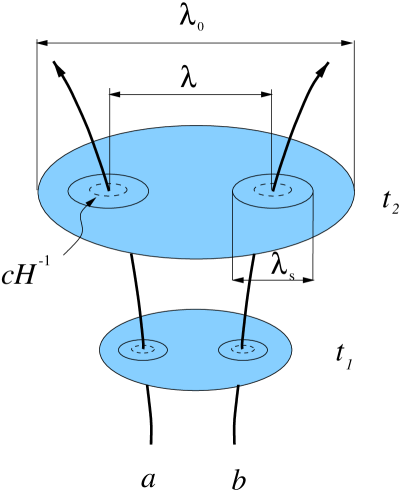
FIG. 1.: A schematic illustration of the separate universes picture, with the symbols as identified in the text.

Consider two such locally homogeneous regions $(a)$ and $(b)$ at fixed spatial coordinates, separated by a coordinate distance $\lambda$, on an initial hypersurface (e.g., uniform-density hypersurface) specified by a fixed coordinate time, $t=t_{1}$, in the appropriate gauge (e.g., uniform-density gauge). The initial large-scale curvature perturbation on the scale $\lambda$ can then be defined (independently of the background) as

$$\delta\psi_{1}\equiv\psi_{a1}-\psi_{b1}\,.$$ (25)

On a subsequent hypersurface defined by $t=t_{2}$ the curvature perturbation at $(a)$ or $(b)$ can be evaluated using Eq. (18) [but neglecting $\nabla^{2}\sigma$] to give [14]

$$\psi_{a2}=\psi_{a1}-\delta N_{a}\,,$$ (26)

where the integrated expansion between the two hypersurfaces along the world-line followed by region $(a)$ is given by $N_{a}=N+\delta N_{a}$, with $N\equiv\ln a$ the expansion in the unperturbed background and

$$\delta N_{a}=\int_{1}^{2}{1\over 3}\delta\tilde{\theta}_{a}dt\,.$$ (27)

The curvature perturbation when $t=t_{2}$ on the comoving scale $\lambda$ is thus given by

$$\delta\psi_{2}\equiv\psi_{a2}-\psi_{b2}=\delta\psi_{1}-\left(N_{a}-N_{b}\right)\,.$$ (28)

In order to calculate the change in the curvature perturbation in any gauge on very large scales it is thus sufficient to evaluate the difference in the integrated expansion between the initial and final hypersurface along different world-lines.

In particular, using Eq. (28), one can evolve the curvature perturbation, $\zeta$, on super-horizon scales, knowing only the evolution of the family of Robertson–Walker universes, which according to the separate Universe assumption describe the evolution of the Universe on super-horizon scales:

$$\Delta\zeta=\Delta N\,,$$ (29)

where $\Delta\zeta=-\psi_{a}+\psi_{b}$ on uniform-density hypersurfaces and $\Delta N=N_{a}-N_{b}$ in Eq. (28). As we shall discuss in the next section, this evolution is in turn specified by the values of the relevant fields during inflation, and as a result one can calculate $\zeta$ at horizon re-entry from the vacuum fluctuations of these fields.

While it is a non-trivial assumption to suppose that every comoving region well outside the horizon evolves like an unperturbed universe, there has to be some scale $\lambda_{\rm s}$ for which that assumption is true to useful accuracy. If there were not, the concept of an unperturbed (Robertson–Walker) background would make no sense. We use the phrase ‘background’ to describe the evolution on a much larger scale $\lambda_{0}$, which should be much bigger even than our present horizon size, with respect to which the perturbations in section II were defined. It is important to distinguish this from regions of size $\lambda_{\rm s}$ large enough to be treated as locally homogeneous, but which when pieced together over a larger scale, $\lambda$, represent the long-wavelength perturbations under consideration. Thus we require a hierarchy of scales:

$$\lambda_{0}\gg\lambda\gg\lambda_{{\rm s}}\gtrsim cH^{-1}\ .$$ (30)

Ideally $\lambda_{0}$ would be taken to be infinite. However it may be that the Universe becomes highly inhomogeneous on some very much larger scale, $\lambda_{{\rm e}}\gg\lambda_{0}$, where effects such as stochastic or eternal inflation determine the dynamical evolution. Nevertheless, this will not prevent us from defining an effectively homogeneous background in our observable Universe, which is governed by the local Einstein equations and hence impervious to anything happening on vast scales. Specifically we will assume that it is possible to foliate spacetime on this large scale $\lambda_{0}$ with spatial hypersurfaces.

When we use homogeneous equations to describe separate regions on length scales greater than $\lambda_{\rm s}$, we are implicitly assuming that the evolution on these scales is independent of shorter wavelength perturbations. This is true within linear perturbation theory in which the evolution of each Fourier mode can be considered independently, but any non-linear interaction introduces mode-mode coupling which undermines the separate universes picture. The separate universe model may still be used for the evolution of linear metric perturbation if the perturbations in the total density and pressure remain small, but a suitable model (possibly a thermodynamic description) of the effect of the non-linear evolution of matter fields on smaller scales may be necessary in some cases. An application to the study of preheating at the end of inflation is discussed in Section V C.

Adiabatic perturbations in the density and pressure correspond to shifts forwards or backwards in time along the background solution, $\delta p/\delta\rho=\dot{p}/\dot{\rho}\equiv c_{s}^{2}$, and hence $\Gamma=0$ in Eq. (13). For example, in a universe containing only baryonic matter plus radiation, the density of baryons or photons may vary locally, but the perturbations are adiabatic if the ratio of photons to baryons remains unperturbed. Different regions are compelled to undergo the same evolution along a unique trajectory in field space, separated only by a shift in the expansion. The pressure $p$ thus remains a unique function of the density $\rho$ and the energy conservation equation, $d\rho/dN=-3(\rho+p)$, determines $\rho$ as a function of the integrated expansion, $N$. Under these conditions, uniform-density hypersurfaces are separated by a uniform expansion and hence the curvature perturbation, $\zeta$, remains constant.

For $\Gamma\neq 0$ it is no longer possible to define a simple shift to describe both the density and pressure perturbation. The existence of a non-zero pressure perturbation on uniform-density hypersurfaces changes the equation of state in different regions of the Universe and hence leads to perturbations in the expansion along different worldlines between uniform-density hypersurfaces. This is consistent with Eq. (20) which quantifies how the non-adiabatic pressure perturbation determines the variation of $\zeta$ on large scales [18, 8].

The entropy perturbation between any two quantities (which are spatially homogeneous in the background) has a naturally gauge-invariant definition [which follows from the obvious extension of Eq. (13)]

$$\Gamma_{xy}\equiv{\delta x\over\dot{x}}-{\delta y\over\dot{y}}\,.$$ (31)

We define a generalized adiabatic condition which requires $\Gamma_{xy}=0$ for any physical scalars $x$ and $y$. In the separate universes picture this condition ensures that if all field perturbations are adiabatic at any one time (i.e. on any spatial hypersurface), then they must remain so at any subsequent time. Purely adiabatic perturbations can never give rise to entropy perturbations on large scales as all fields share the same time shift, $\delta t=\delta x/\dot{x}$, along a single phase-space trajectory.

V Inflation

A Single-component inflaton field

In Section III we showed that the curvature perturbation $\zeta$ on the uniform-density gauge is constant on large scales for adiabatic perturbations. A common application of this is to perturbations produced by a single scalar field during inflation. Even this apparently simple case is somewhat subtle since a scalar field obeys a second-order equation of motion and cannot in general be described by an equation of state $p(\rho)$, since the total energy can be split between potential and kinetic energy. However, the existence of an attractor solution for a strongly-damped inflaton field allows one to drop the decaying mode as inflation progresses and ensures a unique relation between the field value and its first derivative.

The specific relations between the inflaton field and curvature perturbations depends on the choice of gauge. In practice the inflaton field perturbation spectrum can be calculated on uniform-curvature ($\psi=0$) slices, where the field perturbations have the gauge-invariant definition [27, 13]

$$\delta\phi_{\psi}\equiv\delta\phi+{\dot{\phi}\over H}\psi\,.$$ (32)

In the slow-roll limit the amplitude of field fluctuations at horizon crossing ($\lambda=H^{-1}$) is given by $H/2\pi$. Note that this is the amplitude of the asymptotic solution on large scales. This result is independent of the geometry and holds for a massless scalar field in de Sitter spacetime independently of the gravitational field equations.

The field fluctuation is then related to the curvature perturbation on comoving hypersurfaces (on which the scalar field is uniform, $\delta\phi_{c}=0$) using Eq. (7), by

$${\cal R}\equiv\psi_{c}=\frac{H}{\dot{\phi}}\delta\phi_{\psi}\,.$$ (33)

We will now demonstrate that for adiabatic perturbations we can identify the curvature perturbation on comoving hypersurfaces, ${\cal R}$, with the curvature perturbation on uniform-density hypersurfaces, $-\zeta$. In an arbitrary gauge the density and pressure perturbations of a scalar field are given by

$$\delta\rho = \dot{\phi}\,\dot{\delta\phi}-A\dot{\phi}^{2}+V^{\prime}\,\delta\phi\,,$$ (34)

$$\delta p = \dot{\phi}\,\dot{\delta\phi}-A\dot{\phi}^{2}-V^{\prime}\,\delta\phi\,,$$ (35)

where $V^{\prime}\equiv dV/d\phi$. Thus we find $\delta\rho-\delta p=2V^{\prime}\delta\phi$. For adiabatic perturbations on uniform-density hypersurfaces both the density and pressure perturbation must vanish and thus so does the field perturbation $\delta\phi_{\rho}=0$ for $V^{\prime}\neq 0$. Hence the uniform-density and comoving hypersurfaces coincide, and ${\cal R}$ and $-\zeta$ are identical, for adiabatic perturbations.

The asymptotic solution/growing mode for the scalar field vacuum fluctuation corresponds to a perturbation about the background attractor solution and hence generates a purely adiabatic perturbation on super-horizon scales. Thus the density perturbation when a mode re-enters the horizon during the radiation or matter dominated eras can be directly related to the growing mode of the inflaton field perturbation when that mode left the horizon during inflation due to the constancy of $\zeta$ once the decaying mode becomes negligible after horizon crossing [7]. We have shown that this does not depend on any slow-roll type approximation for the inflaton field, nor does it depend on the form of the gravitational field equations. The result holds for any metric theory of gravity that respects local conservation of energy–momentum. As an example, the large-scale curvature perturbation spectrum produced during a period of “brane inflation” has recently been calculated [23] in the four-dimensional effective theory of gravity induced on the world-volume of a 3-brane in five-dimensional Einstein gravity [22, 20], even though the full theory of cosmological perturbations has yet to be determined in this model.

B Multi-component inflaton field

During a period of inflation it is important to distinguish between “light” fields, whose effective mass is less than the Hubble parameter, and “heavy” fields whose mass is greater than the Hubble parameter. Long-wavelength (super-Hubble scale) perturbations of heavy fields are under-damped and oscillate with rapidly decaying amplitude ($\langle\phi^{2}\rangle\propto a^{-3}$) about their vacuum expectation value as the universe expands. Light fields, on the other hand, are over-damped and may decay only slowly towards the minimum of their effective potential. It is the slow-rolling of these light fields that controls the cosmological dynamics during inflation.

The inflaton, defined as the direction of the classical evolution, is one of the light fields, while the other light fields (if any) will be taken to be orthogonal to it in field space. In a multi-component inflation model there is a family of inflaton trajectories, and the effect of the orthogonal perturbations is to shift the inflaton from one trajectory to another.

If all the fields orthogonal to the inflaton are heavy then there is a unique inflaton trajectory in field space. In this case even a curved path in field space, after canonically normalizing the inflaton trajectory, is indistinguishable from the case of a straight trajectory, and leads to no variation in $\zeta$.

When there are multiple light fields evolving during inflation, uncorrelated perturbations in more than one field will lead to different regions that are not simply time translations of each other. In order to specify the evolution of each locally homogeneous universe one needs as initial data the value of every cosmologically significant field. In general, therefore, there will be non-adiabatic perturbations, $\Gamma_{xy}\neq 0$.

If the local integrated expansion, $N$, is sensitive to the value of more than one of the light fields then $\zeta$ is able to evolve on super-horizon scales, as has been shown by several authors [19, 18]. Note also that the comoving and uniform-density hypersurfaces need no longer coincide in the presence of non-adiabatic pressure perturbations. In practice it is necessary to follow the evolution of the perturbations on super-horizon scales in order to calculate the curvature perturbation at later times. In most models studied so far, the trajectories converge to a unique one before the end of inflation, but that need not be the case in general.

The separate universe approach described in section IV gives a rather straightforward procedure for calculating the evolution of the curvature perturbation, $\psi$, on large scales based on the change in the integrated expansion, $N$, in different locally homogeneous regions of the universe. This approach was developed in Refs. [14, 26, 15] for general relativistic models where scalar fields dominate the energy density and pressure, though it has not been applied to many specific models. In the case of a single-component inflaton, this means that on each comoving scale, $\lambda$, the curvature perturbation, $\zeta$, on uniform-density (or comoving) hypersurfaces must stop changing when gradient terms can be neglected ($\lambda>\lambda_{s}$). More generally, with a multi-component inflaton, the perturbations generated in the fields during inflation will still determine the curvature perturbation, $\zeta$, on large scales, but one needs to follow the time evolution during the entire period a scale remains outside the horizon in order to evaluate $\zeta$ at later times. This will certainly require knowledge of the gravitational field equations and may also involve the use of approximations such as the slow-roll approximation to obtain analytic results.

C Preheating

During inflation, every field is supposed to be in the vacuum state well before horizon exit, corresponding to the absence of particles. The vacuum fluctuation cannot play a role in cosmology unless it is converted into a classical perturbation, defined as a quantity which can have a well-defined value on a sufficiently long time-scale [28, 29]. For every light field this conversion occurs at horizon exit ($\lambda\sim H^{-1}$). In contrast, heavy fields become classical, if at all, only when their quantum fluctuation is amplified by some other mechanism.

There has recently been great interest in models where vacuum fluctuations become classical (i.e., particle production occurs) due to the rapid change in the effective mass (and hence the vacuum state) of one or more fields. This usually (though not always [30]) occurs at the end of inflation when the inflaton oscillates about its vacuum expectation value which can lead to parametric amplification of the perturbations — a process which has become known as preheating [2]. The rate of amplification tends to be greatest for long-wavelength modes and this has lead to the claim that rapid amplification of non-adiabatic perturbations could change the curvature perturbation, $\zeta$, even on very large scales [3].

Within the separate universes picture this is certainly possible if preheating leads to different integrated expansion in different regions of the universe. In particular $\zeta$ can evolve if a significant non-adiabatic pressure perturbation is produced on large scales. However it is also apparent in the separate universes picture that no non-adiabatic perturbation can subsequently be introduced on large scales if the original perturbations were purely adiabatic. This is of course also apparent in the field equations where preheating can only amplify pre-existing field fluctuations.

Efficient preheating requires strong coupling between the inflaton and preheating fields which typically leads to the preheating field being heavy during inflation (when the inflaton field is large). The strong suppression of super-horizon scale fluctuations in heavy fields during inflation means that in this case no significant change in $\zeta$ is produced on super-horizon scales before back-reaction due to particle production on much smaller scales damps the oscillation of the inflaton and brings preheating to an end [31, 32, 4].

Because the first-order effect is so strongly suppressed in such models, the dominant effect actually comes from second-order perturbations in the fields [31, 32, 4]. The expansion on large scales is no longer independent of shorter wavelength field perturbations when we consider higher-order terms in the equations of motion. Nonetheless in many cases it is still possible to use linear perturbation theory for the metric perturbations while including second-order perturbations in the matter fields. In Ref. [4] this was done to show that even allowing for second-order field perturbations, there is no significant non-adiabatic pressure perturbation, and hence no change in $\zeta$, on large scales in the original model of preheating in chaotic inflation.

More recently a modified version of preheating has been proposed [33] (requiring a different model of inflation) where the preheating field is light during inflation, and the coupling to the inflaton only becomes strong at the end of inflation. In such a multi-component inflation model non-adiabatic perturbations are no longer suppressed on super-horizon scales and it is possible for the curvature perturbation $\zeta$ to evolve both during inflation and preheating, as described in Section V-B.

VI Conclusions

In this paper, we have identified the general condition under which the super-horizon curvature perturbation on spatial hypersurfaces can vary as being due to differences in the integrated expansion along different worldlines between hypersurfaces. As long as linear perturbation theory is valid, then, when spatial gradients of the perturbations are negligible, such a situation can be described using the separate universes picture, where regions are evolved according to the homogeneous equations of motion.

In particular, the curvature perturbation on uniform-density hypersurfaces, $\zeta$, can vary only in the presence of a significant non-adiabatic pressure perturbation. The result follows directly from the local conservation of energy–momentum and is independent of the gravitational field equations. Thus $\zeta$ is conserved for adiabatic perturbations on sufficiently large scales in any metric theory of gravity, including scalar–tensor theories of gravity or induced four-dimensional gravity in the brane-world scenario.

Multi-component inflaton models are an example where non-adiabatic perturbations may cause the curvature perturbation to evolve on super-horizon scales.

REFERENCES

- [1] A. R. Liddle and D. H. Lyth, Phys. Rep. 231, 1 (1993), astro-ph/9303019.
- [2] L. Kofman, A. Linde, and A. A. Starobinsky, Phys. Rev. D 56, 3258 (1997), hep-ph/9704452.
- [3] B. A. Bassett, D. I. Kaiser, and R. Maartens, Phys. Lett. B 455, 84 (1999), hep-ph/9808404; B. A. Bassett, F. Tamburini, D. I. Kaiser, and R. Maartens, Nucl. Phys. B561, 188 (1999), hep-ph/9901319.
- [4] A. R. Liddle, D. H. Lyth, K. A. Malik and D. Wands, Phys. Rev. D 61, 103508 (2000), hep-ph/9912473.
- [5] J. M. Bardeen, P. J. Steinhardt and M. S. Turner, Phys. Rev. D 28, 679 (1983).
- [6] J. M. Bardeen, in Cosmology and Particle Physics, eds. L. Fang and A. Zee, Gordon and Breach Science Publishers, New York (1988).
- [7] J. Martin and D. J. Schwarz, Phys. Rev. D 57, 3302 (1998).
- [8] D. H. Lyth and A. Riotto, Phys. Rep. 314, 1 (1999), hep-ph/9807278.
- [9] H. Kodama and M. Sasaki, Int. J. Mod. Phys. A 2 491 (1987).
- [10] E. M. Lifshitz, J. Phys. Moscow, 10, 116 (1946).
- [11] J. M. Bardeen, Phys. Rev. D 22, 1882 (1980).
- [12] H. Kodama and M. Sasaki, Prog. Theor. Phys. Suppl. 78, 1 (1984).
- [13] V. F. Mukhanov, H. A. Feldman and R. H. Brandenberger, Phys. Rep. 215, 203 (1992).
- [14] M. Sasaki and E. D. Stewart, Prog. Theor. Phys. 95, 71 (1996), astro-ph/9507001.
- [15] M. Sasaki and T. Tanaka, Prog. Theor. Phys. 99, 763 (1998), gr-qc/9801017.
- [16] J. Hwang, Astrophys. J. 375, 443 (1991).
- [17] J. Hwang, Phys. Rev. D53, 762 (1996), gr-qc/9509044; J. Korean Phys. Soc. 35, S633 (1999), astro-ph/9909150.
- [18] J. García-Bellido and D. Wands, Phys. Rev. D 53, 5437 (1996), astro-ph/9511029.
- [19] A. A. Starobinsky and J. Yokoyama, in Fourth Workshop on General Relativity and Gravitation, ed K. Nakao et al (1995), astro-ph/9502002; J. García-Bellido and D. Wands, Phys. Rev. D 52, 6739 (1995), gr-qc/9506050.
- [20] T. Shiromizu, K. Maeda and M. Sasaki, gr-qc/9910076.
- [21] P. Horava and E. Witten, Nuc. Phys. B 475, 94 (1996, hep-th/9510209; ibid B 460 506 (1996), hep-th/9603142.
- [22] L. Randall and R. Sundrum, Phys. Rev. Lett. 83, 3370 (1999) hep-ph/9905221; Phys. Rev. Lett. 83, 4690 (1999), hep-th/9906064.
- [23] R. Maartens, D. Wands, B. A. Bassett and I. P. C. Heard, to appear in Phys. Rev. D, hep-ph/9912464.
- [24] A. A. Starobinsky, JETP Lett. 42, 51 (1985).
- [25] D. S. Salopek, Phys. Rev. D 52, 5563 (1995), astro-ph/9506146.
- [26] T. Takahiro and E. D. Stewart, Phys. Lett. B381, 413 (1996), astro-ph/9604103.
- [27] V. F. Mukhanov, JETP 68, 1297 (1988).
- [28] A. H. Guth and S.-Y. Pi, Phys. Rev. Lett. 49, 1110, (1982).
- [29] D. H. Lyth, Phys. Rev D 31, 1792 (1985).
- [30] D. J. H. Chung, E. W. Kolb, A. Riotto and I. I. Tkachev, hep-ph/9910437.
- [31] K. Jedamzik and G. Sigl, Phys. Rev. D 61, 023519 (2000), hep-ph/9906287.
- [32] P. Ivanov, Phys. Rev. D 61, 023505 (2000), astro-ph/9906415.
- [33] B. A. Bassett, C. Gordon, R. Maartens and D. I. Kaiser, Phys. Rev. D 61, 061302 (2000), hep-ph/9909482.