The evolution of the stellar populations in low surface brightness galaxies

Abstract

We investigate the star formation history and chemical evolution of low surface brightness (LSB) disk galaxies by modelling their observed spectro-photometric and chemical properties using a galactic chemical and photometric evolution model incorporating a detailed metallicity dependent set of stellar input data. For a large fraction of the LSB galaxies in our sample, observed properties are best explained by models incorporating an exponentially decreasing global star formation rate (SFR) ending at a present-day gas fraction $M_{\rm gas}/(M_{\rm gas}+M_{\rm stars})=0.5$ for a galaxy age of 14 Gyr. For some galaxies small amplitude star formation bursts are required to explain the contribution of the young (5-50 Myr old) stellar population to the galaxy integrated luminosity. This suggests that star formation has proceeded in a stochastic manner.

The presence of an old stellar population in many late-type LSB galaxies suggests that LSB galaxies roughly follow the same evolutionary history as HSB galaxies, except at a much lower rate. In particular, our results imply that LSB galaxies do not form late, nor have a delayed onset of star formation, but simply evolve slowly.

1 Introduction

Deep searches for field galaxies in the local universe have revealed the existence of a large number of galaxies with low surface brightnesses that are hard to detect against the night sky (see the reviews by Impey & Bothun 1997 and Bothun, Impey & McGaugh 1997). Many different kinds of LSB galaxies have so far been found, including giant LSB galaxies (e.g. Sprayberry et al. 1995) and red LSB galaxies (O’Neil et al. 1997), but the most common type seems to be “blue LSB galaxies”: late-type, disk-dominated spirals with central surface brightnesses $\mu_{0}(B)\mathrel{\mathchoice{\vbox{\offinterlineskip\halign{\hfil$\displaystyle#$\hfil\cr>\cr\sim\cr}}}{\vbox{\offinterlineskip\halign{\hfil$\textstyle#$\hfil\cr>\cr\sim\cr}}}{\vbox{\offinterlineskip\halign{\hfil$\scriptstyle#$\hfil\cr>\cr\sim\cr}}}{\vbox{\offinterlineskip\halign{\hfil$\scriptscriptstyle#$\hfil\cr>\cr\sim\cr}}}}23$ mag arcsec^-2.

In this paper, we will concentrate on these late-type LSB spirals. Observations show that they are neither exclusively dwarf systems nor just the faded counterparts of “normal” high surface brightness (HSB) spirals (de Blok et al. 1996, hereafter dB96). In many cases, LSB galaxies follow the trends in galaxy properties found along the Hubble sequence towards very late types. These trends include increasingly blue colours (e.g. Rönnback 1993; McGaugh & Bothun 1994; de Blok et al. 1995 [hereafter dB95]; Bell et al. 1999), decreasing oxygen abundances in the gas (e.g. McGaugh 1994; Rönnback & Bergvall 1995; de Blok & van der Hulst 1998a), and decreasing Hi surface densities (from type Sc onwards; e.g. van der Hulst et al. 1993, hereafter vdH93). Despite the low gas densities, LSB spirals rank among the most gas-rich disk galaxies at a given total luminosity as their Hi disks in general are extended (Zwaan et al. 1995; dB96). The fact that LSB galaxies still have large reservoirs of gas together with their low abundances suggest that the amount of star formation in the past cannot have been very large (vdH93; Van Zee et al. 1997). Clearly, LSB galaxies are not the faded remnants of HSB spirals.

The unevolved nature of LSB spirals can be interpreted in various ways. For instance, LSB spirals could be systems whose stellar population is young and in which the main phase of star formation is still to occur. Alternatively, the stellar population in LSB spirals could be similar to those in HSB galaxies but with a young population dominating the luminosity. This has been explored and modelled in studies by e.g.  Knezek (1993), Jimenez et al. (1998), dB96, Gerritsen & de Blok (1999) and more recently in two papers by Bell et al. (1999) and Bell & de Jong (1999). These studies all indicate a scenario in which LSB galaxies are unevolved systems with low surface densities, low metallicities and a constant or increasing star formation rate (cf. Padoan et al. 1997, however, for a different opinion).

In this paper we address these various scenarios for the evolution of LSB galaxies by detailed modelling of their spectro-photometric and chemical properties. Model results are compared directly with the observed colours, gas phase abundances, gas contents, and current star formation rates of LSB galaxies. Using simple model star formarion histories we confirm the results of previous studies and show that the ratio of young stars to old stars in LSB galaxies is larger than typically found in HSB galaxies.

In reality, however, star formation is unlikely to proceed as smoothly as the various population synthesis models suggest. Gerritsen & de Blok (1999) point out that small surges in the star formation rate are likely to be very important in determining the observed colours of LSB galaxies. In this paper we will pay special attention to the influence of small bursts of star formation on the optical colours, and show that they can have a significant influence on the inferred properties of LSB galaxies.

This paper is organized as follows. We briefly compare observational data of LSB galaxies with those of spirals and dwarf galaxies in Sect. 2. In Sect. 3, we describe the ingredients of the galactic evolution model we used. Some general properties of the model are presented in Sect. 4. The comparison with observational data is presented and discussed in Sect. 5. The impact of small amplitude star formation bursts in LSB galaxies is investigated in Sect. 6 and predicted star formation rates are compared with the observations in Sect. 7. A short discussion of where LSB galaxies fit in the grand scheme of galaxy formation and evolution is presented in Sect. 8. A short summary is given in Sect. 9.

2 Observational characteristics of LSB galaxies

2.1 Sample selection

We use the sample described in dB96. This consists of 24 late-type LSB galaxies (inclinations up to $\sim 60^{\circ}$), taken from the lists by Schombert et al. (1992) and the UGC (Nilson 1973). The sample is representative for the LSB galaxies generally found in the field. We selected a subsample of 16 LSB galaxies for which good data are available. For these systems, optical data have been taken from dB95, Hi data from dB96, and abundance data from McGaugh & Bothun (1994) and de Blok & van der Hulst (1998a).

The galaxy identification and Johnson $UBV$ and Kron-Cousins $RI$ are given in columns (1) to (6) in Table 1 (a Hubble constant of $H_{0}=100$ km s^-1 Mpc^-1 was used). Column (7) lists the $B$-band luminosities; column (8) the Hi-mass-to-light ratio; column (9) and (10) the Hi and dynamical masses respectively. The gas fraction $\mu_{\rm rot}$ in column (11) is given by $M_{\rm gas}$/$(M_{\rm gas}+M_{*,{\rm max}})$ where $M_{*,{\rm max}}$ denotes the mass of the stellar component obtained from maximum disk fitting of the rotation curve (dB96) (see Sect. 2.6). The mean [O/H] abundances are listed in column (12).

Table 1: Observational data on LSB galaxies (de Blok et al. 1995, 1996)

(1)	(2)	(3)	(4)	(5)	(6)	(7)	(8)	(9)	(10)	(11)	(12)
Name	$U$	$B$	$V$	$R$	$I$	$\log L_{B}$	${M_{\rm HI}}\over{L_{B}}$	$\log M_{\rm HI}$	$\log M_{\rm dyn}$	$\mu_{\rm rot}$	[O/H]
F561-1	$-$17.4	$-$17.2	$-$17.8	$-$18.0	$-$18.4	9.08	0.7	8.91	9.66	0.59	$-$0.87
F563-1	$-$16.6	$-$16.7	$-$17.4	$-$17.6	$-$16.4†	8.87	2.0	9.18	10.58	0.19	$-$1.46
F563-V1	$-$15.7	$-$15.7	$-$16.3	$-$16.6†	$-$16.9	8.48	0.9	8.45	9.00	0.59	$-$1.05
F564-V3	*	$-$11.8	$-$12.4	$-$12.6	*	6.91	1.6	7.11	8.80	*	*
F565-V2	*	$-$14.8	$-$15.3	$-$15.6	*	8.11	2.6	8.53	9.58	0.33	*
F567-2	$-$17.0	$-$16.8	$-$17.4	$-$17.4	$-$17.7	8.91	1.5	9.08	9.90	0.49	*
F568-1	$-$17.7	$-$17.5	$-$18.1	$-$18.3	$-$18.8	9.20	1.4	9.34	10.56	0.32	$-$0.98
F568-3	$-$17.8	$-$17.7	$-$18.2	$-$18.5	$-$19.0	9.28	0.8	9.20	10.63	0.45	$-$0.92
F568-V1	$-$17.4	$-$17.3	$-$17.8	$-$18.0	$-$18.5	9.11	1.1	9.15	10.71†	0.53	$-$0.99
F571-5	$-$16.6	$-$16.5	$-$16.9	$-$17.1	*	8.79	*	9.99†	10.45	*	$-$1.53
F571-V1	*	$-$16.4	$-$16.9	$-$17.3	*	8.75	1.2	8.82	10.15	0.33	$-$0.94
F574-2	*	$-$17.0	$-$17.7	$-$17.8	*	8.99	0.9	8.97	9.51	0.66	*
F577-V1	$-$17.9	$-$17.6	$-$18.0	$-$18.1	*	9.23	0.8	9.15	9.20†	*	*
U0128	$-$18.5	$-$18.2	$-$18.7	$-$18.9	$-$19.3	9.48	1.2	9.56	10.86	0.39	*
U0628	$-$18.5	$-$18.5	$-$19.1	$-$19.3	$-$19.7	9.59	*	*	10.69	*	*
U1230	$-$18.9	$-$17.7	$-$18.2	$-$18.5	$-$18.9	9.28	1.7	9.50	10.80	0.60	$-$0.76
Typ. Dwarf	$-$17.5	$-$17	$-$17.5	$-$18	$-$18.5	9.0	1.0	9.0	9.0	0.7	$-$0.6$\pm$0.4
Typ. LSBG	$-$18	$-$17.5	$-$18	$-$18	$-$18.5	9.2	1.3	9.3	10.0	0.5	$-$0.6$\pm$0.4
Typ. HSBG	$-$20	$-$19.5	$-$20	$-$20.5	$-$21	10.0	0.4	9.6	11.0	0.1	$\sim$0.0

* not available, † uncertain

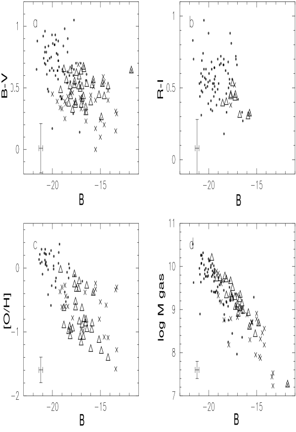
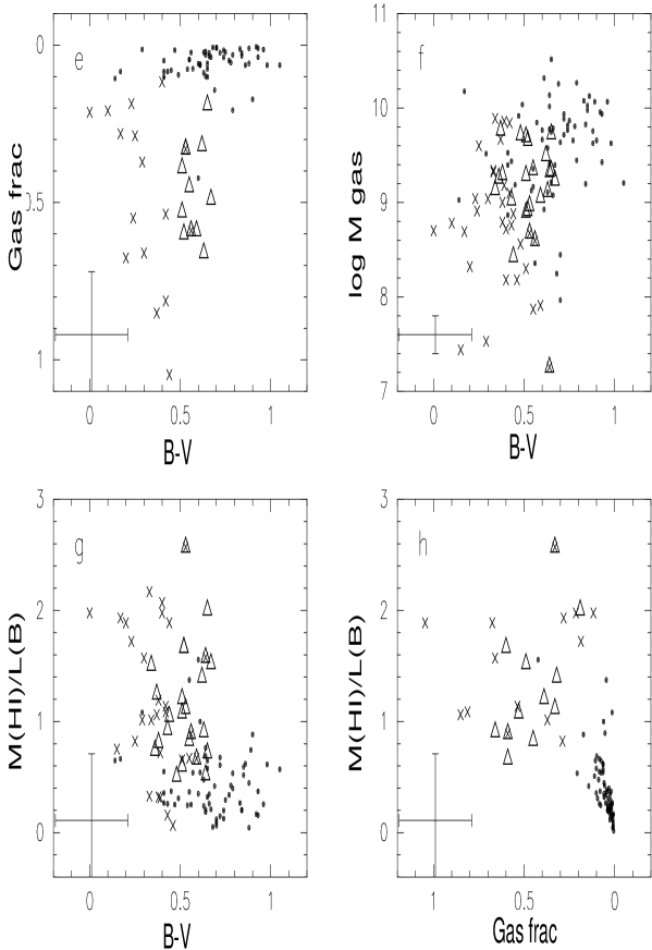
Figure 1: Observational data on LSB galaxies compared to that for normal spirals and dwarf galaxies. Symbols refer to LSB galaxies (triangles; data from de Blok et al. 1995, 1996), normal face-on spirals (full dots; de Jong & van der Kruit 1994), and dwarf galaxies (crosses; Mellise & Israel 1994). LSB galaxies which are probably dwarf systems are indicated by triangles with crosses overlayed. Typical error bars are indicated in the bottom left of each panel.

2.2 Magnitudes and colours

We compare in Fig. 1$a$ and $b$ magnitudes and broadband colours of LSB galaxies to those of late-type HSB face-on spirals (de Jong & van der Kruit 1994) and dwarf galaxies (Melisse & Israel 1994; Gallagher & Hunter 1986, 1987). The usual distinction between HSB and LSB galaxies is purely an artificial one since normal galaxies along the Hubble sequence show a continuous range in central surface brightness, i.e. ranging from values around the Freeman value for early type systems to the very faint values observed for the late-type LSB galaxies in our sample (e.g. de Jong 1995; dB95). For the purpose of this paper we will continue to use the distinction as a shorthand, where “HSB galaxy” should be interpreted as “typical Hubble sequence Sc galaxy.” Fig. 1$a$ and $b$ show that LSB galaxies are generally bluer and fainter than their HSB counterparts (e.g. McGaugh 1992; vdH93; dB95).

2.3 Abundances

Estimates of the ISM abundances in LSB galaxies predominantly rely on abundance determinations of their Hii regions. Oxygen abundances of Hii regions listed in Table 1 are taken from McGaugh (1994) and de Blok & van der Hulst (1998a).

We assume that the Hii-region abundances on average are a reasonable indicator of the ISM abundances within a given LSB spiral. The intrinsic scatter in [O/H] among different Hii regions within a given LSB galaxy is usually of the order 0.2 dex (e.g. McGaugh 1994). Bell & de Jong (1999) find that the gas metal abundances in LSB galaxies generally trace the stellar metallicities quite well, with the stars being $\sim 0.4$ dex more metal-poor.

In Fig. 1c we compare mean [O/H] abundances of Hii regions in LSB galaxies with those in HSB spirals (Zaritsky et al. 1994) and dwarf galaxies (Melisse & Israel 1994; Gallagher & Hunter 1986, 1987). On average, LSB galaxies generally follow the correlation between the characteristic gas-phase abundance and luminosity as found for HSB spirals (Zaritsky et al. 1994), but with a large scatter. The range in [O/H] at a given $B$ magnitude is nearly one dex. This scatter is probably related to evolutionary differences among the LSB galaxies of a given $B$ magnitude (e.g. in the ratio of old to young stellar populations) and/or the Hii regions they contain.

2.4 Extinction

Observational studies by (amongst others) Bosma et al. (1992), Byun (1992), Tully & Verheijen (1997) show that late-type spirals appear transparent throughout their disks. This supports the idea that face-on extinction in LSB galaxies is relatively low, i.e. $E_{B-V}\mathrel{\mathchoice{\vbox{\offinterlineskip\halign{\hfil$\displaystyle#$\hfil\cr<\cr\sim\cr}}}{\vbox{\offinterlineskip\halign{\hfil$\textstyle#$\hfil\cr<\cr\sim\cr}}}{\vbox{\offinterlineskip\halign{\hfil$\scriptstyle#$\hfil\cr<\cr\sim\cr}}}{\vbox{\offinterlineskip\halign{\hfil$\scriptscriptstyle#$\hfil\cr<\cr\sim\cr}}}}0.1$ (e.g. McGaugh 1994). This is consistent with findings by Tully & Verheijen (1998), who studied a large sample of galaxies in the UMa cluster and found the LSB galaxies in their sample to be transparent, whereas non-negligible extinction was present in the HSB galaxies.

In this study we will ignore the possible effects of dust on the colours and magnitudes. See Sect. 5.3 for a discussion.

2.5 Gas masses

We compare in Fig. 1d the observed atomic gas masses $M_{\rm g}\sim 1.4M_{\rm HI}$ (corrected for helium) of LSB galaxies with those of HSB galaxies and dwarfs. Strictly speaking we should also take the molecular gas mass into account. However, so far no CO-emission has been detected in late-type LSB galaxies (Schombert et al. 1990; de Blok & van der Hulst 1998b, but see Knezek 1993 for a discussion on giant LSB galaxies). The amount of molecular gas in LSB galaxies is probably small, even though relatively high CO/H₂ conversion factors may apply in these low metallicity galaxies (Wilson 1995, Mihos et al. 1999). We conclude that, on average, LSB galaxies are considerably more gas-rich (up to a factor $\sim 3$) than HSB galaxies of the same $B$ magnitude (see also Fig. 1g).

2.6 Gas fractions and mass-to-light ratios

We show in Figs. 1g and h the distribution of the mass-to-light ratio $M_{\rm HI}/L_{B}$ vs $(B-V)$ and vs $\mu_{rot}$, respectively. LSB galaxies exhibit considerably higher $M_{\rm HI}/L_{B}$ ratios than HSB spirals (cf. Table 1 and McGaugh & de Blok 1997).

We would however like to know the ratio of gas mass to stellar mass, i.e. the gas fraction $\mu_{1}\equiv M_{\rm gas}$ / $(M_{\rm gas}+M_{\rm stars}$ of a galaxy. This involves the conversion of the observed galaxy luminosity to stellar mass. However, the mass-to-light ratio of the underlying stellar population is generally not well known and, in fact, is an important quantity to determine. Assuming a fixed value of the mass-to-light ratio will however introduce artificial trends since this ratio is expected to vary among galaxies having different star formation histories (e.g. Larson & Tinsley 1978).

As a partial solution we have determined the gas fraction $\mu_{\rm rot}\equiv M_{\rm gas}/(M_{\rm gas}+M_{*,{\rm max}})$ where $M_{*,{\rm max}}$ denotes the mass of the stellar component obtained from maximum disk fitting of the rotation curve (dB96). This method likely overestimates the contribution of the luminous stellar disk to the observed total mass distribution by about a factor of 2 (e.g. Kuijken & Gilmore 1989; Bottema 1995) and, therefore, also provides a lower limit to the actual gas fraction. In summary, while $\mu_{1}$ is a model quantity, $\mu_{\rm rot}$ is determined from observations.

Figs. 1e and 1f show the distribution of the present-day gas fraction $\mu_{\rm rot}$ and total gas mass vs $(B-V)$. It can be seen that LSB galaxies and dwarfs exhibit larger gas fractions than HSB spirals. Taking into account the factor of $\sim 2$ overestimate, values for LSB galaxies are typically $\mu_{1}\mathrel{\mathchoice{\vbox{\offinterlineskip\halign{\hfil$\displaystyle#$\hfil\cr>\cr\sim\cr}}}{\vbox{\offinterlineskip\halign{\hfil$\textstyle#$\hfil\cr>\cr\sim\cr}}}{\vbox{\offinterlineskip\halign{\hfil$\scriptstyle#$\hfil\cr>\cr\sim\cr}}}{\vbox{\offinterlineskip\halign{\hfil$\scriptscriptstyle#$\hfil\cr>\cr\sim\cr}}}}0.5$ and $\mu_{1}\sim 0.1$ for HSB spirals.

We conclude that the available evidence supports of the view that LSB galaxies are relatively unevolved systems compared to HSB spirals. This agrees well with the fact that LSB galaxies usually display properties intermediate to those of HSB spirals and dwarf galaxies.

3 Model description and assumptions

We here summarise the galactic evolution model used (for a more extensive description see van den Hoek 1997, hereafter vdH97). We concentrate on the stellar contribution to the total galaxy luminosity in a given passband (other contributions are neglected). For a given star formation history (SFH), we compute the chemical enrichment of a model galaxy by successive generations of evolving stars. To derive the stellar luminosity in a given passband at a given age, we use a metallicity dependent set of theoretical stellar isochrones as well as a library of spectro-photometric data.

3.1 Chemical evolution model

We start from a model galaxy initially devoid of stars. We follow the chemical enrichment during its evolution assuming stars to be formed according to a given star formation rate (SFR) and initial mass function (e.g. a power law IMF: d$N$/d$m\equiv M(m)\propto m^{\gamma}$). Both stellar and interstellar abundances as a function of galactic evolution time $t_{ev}$ are computed assuming that the stellar ejecta are returned and homogeneously mixed to the ISM at the end of the individual stellar lifetimes (i.e. relaxing the instantaneous recycling approximation; see Searle & Sargent 1972). A description of the set of galactic chemical evolution equations used can be found in e.g. Tinsley (1980) and Twarog (1980), see also vdH97. This model is a closed-box model.

We follow the stellar enrichment of the star forming galaxy in terms of the characteristic element contributions of Asymptotic Giant Branch (AGB) stars, SNII and SNIa. This treatment is justified by the specific abundance patterns observed within the ejecta of these stellar groups (see e.g. Trimble 1991; Russell & Dopita 1992). A detailed description of the metallicity dependent stellar lifetimes, element yields, and remnant masses is given by vdH97 and van den Hoek & Groenewegen (1997). We compute the abundances of H, He, O, and Fe, as well as the heavy element integrated metal-abundance $Z$ (for elements more massive than helium), during the evolution of the model galaxy. Both the SFH, IMF and resulting element abundances as a function of galactic evolution time are used as input for the spectro-photometric evolution model described below.

Boundary conditions to the chemical evolution model are the galaxy total mass $M_{\rm tot}$, its evolution time $t_{\rm ev}$, and the initial gas abundances. Note that solutions of the galactic chemical evolution equations are independent of the ratio of the SFR normalisation and $M_{\rm tot}$. Primordial helium and hydrogen abundances are adopted as $Y_{\rm p}=0.232$ and $X=0.768$ (cf. Pagel & Kazlauskas 1992). Initial abundances for elements heavier than helium are initially set to zero.

Table 2: Parameters related to IMF and stellar enrichment

$\gamma$	$-$2.35	slope of power-law IMF
$(m_{\rm l}$, $m_{\rm u})$	(0.1, 60) $M_{\odot}$	stellar mass range at birth
$(m_{\rm l}^{\rm AGB}$, $m_{\rm u}^{\rm AGB})$	(0.8, 8) $M_{\odot}$	progenitor mass range for AGB stars
$(m_{\rm l}^{\rm SNII}$, $m_{\rm u}^{\rm SNII})$	(8, 30) $M_{\odot}$	progenitor mass range for SNII
$(m_{\rm l}^{\rm SNIa}$, $m_{\rm u}^{\rm SNIa})$	(2.5, 8) $M_{\odot}$	progenitor mass range for SNIa
$\nu^{\rm SNIa}$	0.015	fraction of progenitors ending as SNIa

We list the main input parameters in Table 2, i.e. the adopted IMF-slope, minimum and maximum stellar mass limits at birth as well as the progenitor mass ranges for stars ending their lives as AGB star, SNIa, and SNII, respectively. For simplicity, we assume the stellar yields of SNIb,c to be similar to those of SNII. Furthermore, we assume a fraction $\nu^{\rm SNIa}=0.015$ of all white dwarf progenitors with initial masses between $\sim 2.5$ and 8 $M_{\odot}$ to end as SNIa. These and other particular choices for the enrichment by massive stars are based on similar models recently applied to the chemical evolution of the Galactic disk (e.g. Groenewegen et al. 1995; vdH97).

3.2 Spectro-photometric evolution model

The total luminosity of a galaxy in a wavelength interval $\Delta\lambda$ is determined by: 1) the stellar contribution $L_{\rm*}$, 2) the ISM contribution $L_{\rm ism}$ (e.g. Hii-regions, high-energy stellar outflow phenomena, etc.), and 3) the contribution due to absorption and scattering $L_{\rm ext}$:

$$L_{\rm gal}^{\Delta\lambda}(t)=L_{\rm*}+L_{\rm ism}-L_{\rm ext}$$ (1)

where each term in general is a complex function of galactic evolution time. We concentrate on the stellar contribution and neglect the last two terms in Eq. (1). Then, the luminosity in a wavelength interval $\Delta\lambda$ at galactic evolution time $t=T$ can be written as:

$$L_{\rm gal}^{\Delta\lambda}(t={T})=$$ (2)

$$\int_{t=0}^{T}\int_{m_{\rm l}}^{m_{\rm o}({T}-t)} L_{\rm*}^{\Delta\lambda}(m,Z(t),{T}-t)S(t)M(m){\rm d}m{\rm d}t$$

where $m_{\rm l}$ denotes the lower stellar mass limit at birth, $m_{\rm o}(t)$ the turnoff mass for stars evolving to their remnant stage at evolution time $t_{\rm ev}$, and $L_{\rm*}^{\Delta\lambda}$ the luminosity of a star with initial mass $m$, initial metallicity $Z(t)$, and age ($T-t$). We assume a separable SFR: $S(m,t)=S(t)M(m)$ where $S(t)$ is the star formation rate by number [yr^-1] and $M(m)$ the IMF [$M_{\odot}$^-1]. By convention, we normalise the IMF as $\int M(m){\rm d}m=1$ where the integration is over the entire stellar mass range [$m_{\rm l}$, $m_{\rm u}$] at birth (cf. Table 2).

Starting from the chemical evolution model described above, we compute the star formation history $S(m,t)$, gas-to-total mass-ratio $\mu(t)$, and age-metallicity relations (AMR) $Z_{i}(t)$ for different elements $i$. Thus, at each galactic evolution time $t_{\rm ev}$ the ages and metallicities of previously formed stellar generations are known. To derive the stellar passband luminosity $L_{\rm*}^{\Delta\lambda}$ we use a set of theoretical stellar isochrones, as well as a library of spectro-photometric data. Stellar evolution tracks provide the stellar bolometric luminosity $L_{\rm*}^{\rm bol}$, effective temperature $T_{\rm eff}$, and gravity $g$, as a function of stellar age for stars with initial mass $m$ born with metallicity $Z_{\rm*}$. We compute Eq. (2) using a spectro-photometric library containing the stellar passband luminosities $L_{\rm*}^{\Delta\lambda}$ tabulated as a function of $T_{\rm eff}$, $\log g$, and $Z_{\rm*}$ (see below).

The turnoff mass $m_{\rm o}({T}-t)$ occuring in Eq. (2) depends on the metallicity $Z(t)$ of stars formed at galactic evolution time $t_{\rm ev}$. For instance, the turnoff mass for stars born with metallicity $Z=10^{-3}$ at a galactic age of $t_{\rm ev}=14$ Gyr is $m_{\rm o}\sim 0.8$ $M_{\odot}$ (e.g. Schaller et al. 1992). This value differs considerably from $m_{\rm o}\sim 0.95$ $M_{\odot}$ for stars born with metallicity $Z=Z_{\odot}$. Such differences in $m_{\rm o}$ affect the detailed spectro-photometric evolution of a galaxy by constraining the mass-range of stars in a given evolutionary phase (e.g. horizontal branch) at a given galactic evolution time. In the models described below, we explicitly take into account the dependence of $m_{\rm o}(t)$ on the initial stellar metallicity $Z_{*}$ (see vdH97)

Figure 2: Theoretical star formation histories (left) and resulting [O/H] vs age relations (right): constant SFR (thick solid line), linear decrease (thin solid), exponential decrease (dashed; $\tau_{\rm sfr}=5$ Gyr), fast exponential decrease (dotted; $\tau_{\rm sfr}=4$ Gyr), linear increase (dash-dotted), exponential increase (dot-dashed). SFRs have been normalised to a current gas-to-total mass-ratio $\mu_{1}=0.1$.

Figure 3: Exponentially decreasing SFR model: total number of stars formed (left) and average stellar bolometric luminosity (right) vs galactic age for different evolutionary phases: MS (solid curve), RGB (dashed), HB (dot-dashed), EAGB (dotted), and AGB (dash-dotted).

Figure 4: Photometric evolution of exponentially decreasing SFR (top panels) and constant SFR (bottom) models. Left panels: $B$-mag contribution for stars in different evolutionary phases as in Fig. 3: MS (solid curve), RGB (dashed), HB (dot-dashed), EAGB (dotted), AGB (dash-dotted), and Total (thick solid). Right panels: Same as left panels but for $I$-mag

3.3 Stellar evolution tracks and spectro-photometric data

We use the theoretical stellar evolution tracks from the Geneva group (e.g. Schaller et al. 1992; Schaerer et al. 1993). These uniform grids cover large ranges in initial stellar mass and metallicity, i.e. $m=0.05-120$ $M_{\odot}$ and $Z=0.04-0.001$, respectively. These tracks imply a revised solar metallicity of $Z_{\odot}=0.0188$ with $Y_{\odot}=0.299$, and $\Delta Y/\Delta Z=3.0$ for a primordial He-abundance of $Y_{\rm p}=0.232$. For stars with $m>7$ $M_{\odot}$, these tracks were computed until the end of central C-burning, for stars with $m=2-5$ $M_{\odot}$ up to the early-AGB, and for $m<1.7$ $M_{\odot}$ up to the He-flash. For stars with $m\mathrel{\mathchoice{\vbox{\offinterlineskip\halign{\hfil$\displaystyle#$\hfil\cr<\cr\sim\cr}}}{\vbox{\offinterlineskip\halign{\hfil$\textstyle#$\hfil\cr<\cr\sim\cr}}}{\vbox{\offinterlineskip\halign{\hfil$\scriptstyle#$\hfil\cr<\cr\sim\cr}}}{\vbox{\offinterlineskip\halign{\hfil$\scriptscriptstyle#$\hfil\cr<\cr\sim\cr}}}}0.8$ $M_{\odot}$, we used the stellar isochrone program from the Geneva group (Maeder & Meynet, priv. comm.; see also vdH97 ).

To cover the latest stellar evolutionary phases (i.e. horizontal branch (HB), early-AGB, and AGB) for stars with $m\mathrel{\mathchoice{\vbox{\offinterlineskip\halign{\hfil$\displaystyle#$\hfil\cr<\cr\sim\cr}}}{\vbox{\offinterlineskip\halign{\hfil$\textstyle#$\hfil\cr<\cr\sim\cr}}}{\vbox{\offinterlineskip\halign{\hfil$\scriptstyle#$\hfil\cr<\cr\sim\cr}}}{\vbox{\offinterlineskip\halign{\hfil$\scriptscriptstyle#$\hfil\cr<\cr\sim\cr}}}}8$ $M_{\odot}$, we extended the tracks from Schaller et al. with those from Lattanzio (1991; HB and early-AGB) for $m\sim 1-2$ $M_{\odot}$, and from Groenewegen & de Jong (1993; early-AGB and AGB) for $m\sim 1-8$ $M_{\odot}$. These tracks roughly cover the same metallicity range as the tracks from the Geneva group. Corresponding isochrones were computed on a logarithmic grid of stellar ages, covering galactic evolution times up to $t_{\rm ev}\sim 14$ Gyr. Isochrones are linearly interpolated in $m$, log $Z$, and log $t$.

The spectro-photometric data library that we use is based on the Revised Yale Isochrones and has been described extensively by Green et al. (1987). These data include stellar $UBVRI$ Johnson-Cousins magnitudes covering the following ranges in $T_{\rm eff}[{\rm K}]=2800$ to 20000, log $g$ [cm s^-2] $=-0.5$ to 6, and log ($Z/{Z}_{\odot})\sim-2.5$ to $+0.5$. Corresponding spectro-photometric data for stars with $T_{\rm eff}>20000$ K have been adopted from Kurucz (1979) at solar metallicity, covering $T_{\rm eff}=20000-50000$ K.

Although a detailed description of the tuning and calibration of the adopted photometric model is beyond the scope of this paper, we note that the model has been checked against various observations including integrated colours and magnitudes, luminosity functions, and colour-magnitude diagrams of Galactic and Magellanic Cloud open and globular clusters covering a wide range in age and metallicity (see vdH97).

4 General properties of the model

Before discussing the modelling of LSB galaxies, we first describe the general behaviour of the models assuming a few different star formation scenarios.

We start from a model galaxy with initial mass $M_{\rm g}(t=0)=10^{10}$ $M_{\odot}$, initially metal-free and devoid of stars. The chemical and photometric evolution of this galaxy is followed during an evolution time $t_{\rm ev}=14$ Gyr, assuming one of the theoretical star formation histories discussed below. Unless stated otherwise, we assume that stars are formed according to a Salpeter (1955) IMF (i.e. $\gamma=-2.35$) with stellar mass limits at birth between 0.1 and 60 $M_{\odot}$ (cf. Table 2).

Table 3: Star formation models ($\mu_{1}=0.1$ and $M_{\rm tot}=10^{10}$ $M_{\odot}$, unless noted otherwise)

(1)	(2)	(3)	(4)	(5)	(6)	(7)	(8)	(9)	(10)	(11)
	Model	$\langle$SFR$\rangle$	SFR1	$\alpha$	[O/H]1	$N_{\rm tot}$	$L_{B}$	$M_{\rm HI}/L_{B}$	$\gamma$	Notes
		[$M_{\odot}$yr-1]				$[\times 10^{10}]$	[$\times 10^{9}L_{\odot,{B}}$]	[$M_{\odot}/L_{\odot,{B}}$]
A1	Exp. decreasing	0.93	0.17	0.18	+0.3	3.6	3.6	0.16	$-2.35$	(a)
A2	”	0.52	0.09	0.18	$-$0.25	2.1	2.3	1.56	$-2.35$	(a, b)
A3	”	0.69	0.13	0.18	$-$0.9	4.7	1.6	0.45	$-3$	(a)
B1	Constant	0.89	0.89	1.0	+0.3	3.4	10	0.03	$-2.35$
B2	”	0.49	0.49	1.0	$-$0.25	2.1	6.4	0.58	$-2.35$	(b)
B3	”	0.68	0.68	1.0	$-$0.9	4.7	3.7	0.21	$-3$
C	Exp. decreasing	0.90	0.07	0.08	+0.3	11	2.3	0.32	$-2.35$	(c)
D	Lin. decreasing	0.90	0.60	0.67	+0.3	3.5	7.6	0.10	$-2.35$
E	Exp. increasing	0.85	3.06	3.4	+0.3	3.3	28	0.03	$-2.35$
F	Lin. increasing	0.87	1.74	2.0	+0.3	3.3	18	0.04	$-2.35$

Notes: (a) $\tau_{\rm sfr}=5$ Gyr. (b) $\mu_{1}=0.5$. (c) $\tau_{\rm sfr}=4$ Gyr

The following star formation histories are considered: 1) constant, 2) exponentially decreasing, 3) linearly decreasing, 4) exponentially increasing, and 5) linearly increasing. Normalised SFRs and resulting age-ISM metallicity relations are shown in Fig. 2. For each model, the amplitude of the SFR is chosen such that a present-day gas-to-total mass-ratio $\mu_{1}=0.1$ is achieved.

In columns (2) to (6) of Table 3, we list the functional form of the SFR, average past and current SFRs, the ratio of current and average past SFRs $\alpha$, and the present-day mass averaged ISM oxygen abundance. The average past SFR is roughly the same for all models ending at $\mu_{1}=0.1$ and is $\langle$SFR$\rangle=0.9$ $M_{\odot}$yr^-1. In contrast, present-day SFRs range from SFR₁ = 0.07 to 3 $M_{\odot}$yr^-1 and in fact determine the contribution by young stars to the integrated light of the model galaxy. Current oxygen abundances predicted are [O/H]${}_{1}\sim+0.25$ and are mainly determined by $\mu_{1}$, the IMF, and the assumed mass limits for SNII (cf. Table 3). Column (7) gives the number of stars formed, Column (8) their total $B$ band luminosity. Column (10) shows the resulting Hi mass-to-light ratio. Column (11) gives the slope of the IMF used, while Column (11) refers to additional Notes.

Let us consider the photometric evolution of the constant and exponentially decreasing SFR models in some more detail. Fig. 3 shows the evolution of the total number of MS and post-MS stars for exponentially decreasing SFR model A1. The current total number of MS stars is roughly $4\cdot 10^{10}$, compared to $\sim 10^{8}$ post-MS stars (all phases) and $\sim 3\cdot 10^{4}$ for AGB stars only. The present-day mean luminosity of stars on the MS is $\sim 10^{-1}\ L_{\odot}$ compared to $\sim 10^{4}\ L_{\odot}$ for AGB stars. The current bolometric galaxy luminosity is determined mainly by MS stars ($L_{\rm MS}\sim 4\cdot 10^{9}\ L_{\odot}$). In particular, AGB stars ($L_{\rm AGB}\sim 10^{8}\ L_{\odot}$) are relatively unimportant.

Figure 5: Broadband colours vs galactic age for exponentially decreasing SFR (thick solid) and constant SFR (solid) models. Note the different magnitude scales in the upper two and bottom three panels, respectively.

We show in Fig. 4 the $B$ and $I$-band magnitudes of stars in different evolutionary phases (again for the exponential model). As for the bolometric galaxy luminosity, MS stars generally dominate in the $B$-band. However, in the $I$-band, RGB and HB stars are nearly as important as MS stars, at least in later stages of galactic evolution. Due to the cooling of old, low-mass MS stars as well as the increasing contribution by RGB and HB stars with age, the current total $I$-band magnitude is considerably brighter than that in the B-band. This qualitative model behaviour is insensitive to the adopted star formation history (for e-folding times larger than $3-5$ Gyr) but instead is determined by the assumed IMF and the stellar input data used. Thus, constant star formation models exhibit a similar behaviour apart from being brighter by about one magnitude in all passbands at late times (cf. Fig. 4).

Fig. 5 illustrates the sensitivity of broadband colours to the star formation history for constant and exponentially decreasing SFR models. The colours considered here redden with galactic age. In general, differences between colours such as for different SFR models are less than the variations of these colours with age for a given model. Assuming a galactic age of e.g. 8 instead of 14 Gyr has limited effect on the resulting galaxy colours (e.g. less than 0.1 mag in $B-V$), even though absolute magnitudes are substantially altered. Both age and extinction effects can result in substantial reddening of the colours of a stellar population in almost the same manner and it is difficult to disentangle their effects on the basis of photometry data alone. Clearly, galaxy colours alone are not well suited to discriminate between different SFR models, even when internal extinction is low and other reddening effects are negligible (see below).

5 Results

As our emphasis will be on a comparison between the evolution of HSB and LSB galaxies, we will first focus on the relatively well-known evolution of HSB galaxies, using a model chosen to emphasise the observed properties of HSB galaxies. Using this as a starting point, we explore other models to find the best model for LSB galaxies.

5.1 HSB galaxies: $\mu_{1}=0.1$ models

Models using exponentially decreasing SFRs and different e-folding times for different Hubble types (e.g. Larson & Tinsley 1978; Guiderdoni & Rocca-Volmerange 1987; Kennicutt 1989; Bruzual & Charlot 1993; Fritze-v. Alvensleben & Gerhard 1994) are usually found to be in good agreement with observations of HSB galaxies. Therefore we will mainly focus on the exponential SFR models discussed above. As the gas-richness is one of the obvious differences between HSB and LSB galaxies, we will first focus on models with $\mu_{1}=0.1$ to describe HSB galaxies.

Fig. 6 shows the results of the exponentially decreasing SFR model: SFR $\propto\exp(-t/\tau_{\rm sfr})$ with $\tau_{\rm sfr}=5$ Gyr ending at $\mu_{1}=0.1$ at $t=t_{ev}=14$ Gyr for several initial galaxy masses $M_{\rm g}(t=0)\sim 10^{8}-10^{10}$ $M_{\odot}$. The precise value of $\mu_{1}$ was achieved by scaling the amplitude of the SFR accordingly. Galaxy colours and abundances are not affected by this scaling while absolute magnitudes and final gas masses scale with $M_{\rm g}(t=0)$ (as indicated in Fig. 6).

Present-day ($B-V$) and ($R-I$) colours for this model are 0.6 and 0.5, respectively. HSB galaxies with $(B-V)\mathrel{\mathchoice{\vbox{\offinterlineskip\halign{\hfil$\displaystyle#$\hfil\cr>\cr\sim\cr}}}{\vbox{\offinterlineskip\halign{\hfil$\textstyle#$\hfil\cr>\cr\sim\cr}}}{\vbox{\offinterlineskip\halign{\hfil$\scriptstyle#$\hfil\cr>\cr\sim\cr}}}{\vbox{\offinterlineskip\halign{\hfil$\scriptscriptstyle#$\hfil\cr>\cr\sim\cr}}}}0.6$ and $(R-I)\mathrel{\mathchoice{\vbox{\offinterlineskip\halign{\hfil$\displaystyle#$\hfil\cr>\cr\sim\cr}}}{\vbox{\offinterlineskip\halign{\hfil$\textstyle#$\hfil\cr>\cr\sim\cr}}}{\vbox{\offinterlineskip\halign{\hfil$\scriptstyle#$\hfil\cr>\cr\sim\cr}}}{\vbox{\offinterlineskip\halign{\hfil$\scriptscriptstyle#$\hfil\cr>\cr\sim\cr}}}}0.5$ can be explained only when substantial amounts of internal dust extinction are incorporated. The reason is that even though a single stellar population born with metallicity $Z=0.02$ may become as red as $(B-V)\sim 1.1$ and $(R-I)\sim 0.8$, the luminosity contribution by young stellar populations (with ages less than a few Gyr) results in substantial blueing of the galaxy colours. For the same reason, values of $(B-V)\mathrel{\mathchoice{\vbox{\offinterlineskip\halign{\hfil$\displaystyle#$\hfil\cr>\cr\sim\cr}}}{\vbox{\offinterlineskip\halign{\hfil$\textstyle#$\hfil\cr>\cr\sim\cr}}}{\vbox{\offinterlineskip\halign{\hfil$\scriptstyle#$\hfil\cr>\cr\sim\cr}}}{\vbox{\offinterlineskip\halign{\hfil$\scriptscriptstyle#$\hfil\cr>\cr\sim\cr}}}}0.65$ are not predicted by dust-free models independent of the adopted (exponential) SFR (as long as $\tau\mathrel{\mathchoice{\vbox{\offinterlineskip\halign{\hfil$\displaystyle#$\hfil\cr>\cr\sim\cr}}}{\vbox{\offinterlineskip\halign{\hfil$\textstyle#$\hfil\cr>\cr\sim\cr}}}{\vbox{\offinterlineskip\halign{\hfil$\scriptstyle#$\hfil\cr>\cr\sim\cr}}}{\vbox{\offinterlineskip\halign{\hfil$\scriptscriptstyle#$\hfil\cr>\cr\sim\cr}}}}4$ Gyr) or IMF. Therefore, considerable reddening of the younger stellar populations is required to explain the colours of HSB galaxies in this model. Figs. 6c and d show that both the [O/H] abundance ratios and present-day gas masses of HSB galaxies can be explained reasonably well for $M_{\rm g}(t=0)>10^{10}$ $M_{\odot}$. These conclusions agree with results from many previous models (with different stellar input data) for HSB galaxies (e.g. Larson & Tinsley 1978; Guiderdoni & Rocca-Volmerange 1987).

It is clear from Fig. 6 that this model is not able to explain the properties of the LSB galaxies in our sample. The model colours are too red while the predicted [O/H] abundances are too high. As LSB galaxies have higher gas-fractions we thus need to broaden the range of gas-fractions.

5.2 LSB galaxies: $\mu_{1}\neq 0.1$ models

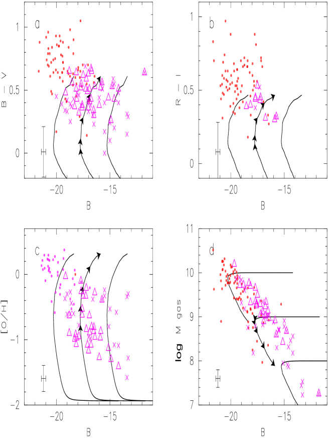
Figure 6: Exponentially decaying SFR model A1: photometric and chemical evolution results. Curves have been drawn for initial galaxy masses $M_{\rm g}(t=0)=10^{8}$, $10^{9}$, and $10^{10}$ $M_{\odot}$. For the $M_{\rm g}(t=0)=10^{9}$ $M_{\odot}$ model, arrows indicate evolution times of 1, 2, 4, 8, and 14 Gyr, respectively. Symbols refer to the following galaxy samples: face-on HSB spirals (dots; de Jong & van der Kruit 1994), LSB spiral galaxies (triangles; de Blok et al. 1995), and dwarf irregulars (crosses; Melisse and Israel 1994). Typical observational errors are shown in the bottom left of each panel.

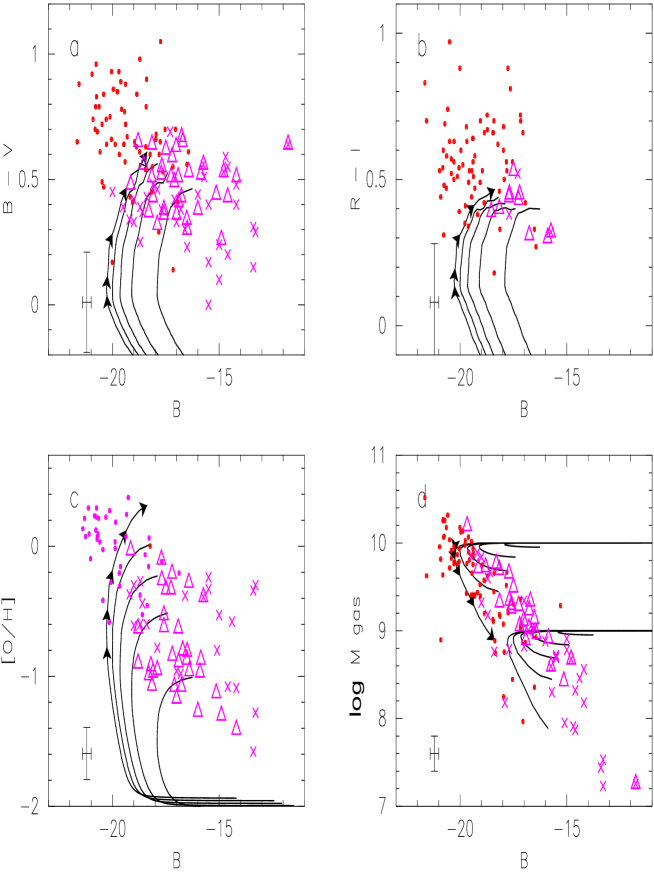
Figure 7: Photometric and chemical evolution results in case of exponentially decaying SFR models ending at $\mu_{1}=$ 0.025, 0.3, 0.5, 0.7, and 0.9 for an initial galaxy mass of $M_{\rm g}(t=0)=10^{10}$ $M_{\odot}$ (in Fig.7̃d we show also results for $M_{\rm g}(t=0)=10^{9}$ $M_{\odot}$). Arrows on top of the $\mu_{1}=0.025$ model indicate evolution times of 1, 2, 4, 8, and 14 Gyr, respectively. Observational data as in Fig. 6

We now consider models with gas fractions $\mu_{1}=$ 0.025, 0.1, 0.3, 0.5, 0.7, and 0.9. First we will examine the constraints which individual properties such as abundance and gas-fraction impose on the models, before combining these in a final model.

5.2.1 Colours and magnitudes

Results for a model with initial mass $M_{\rm g}(t=0)=10^{10}$ $M_{\odot}$ are shown in Fig. 7. While the age distribution of the stellar populations is identical in all the models shown, present-day ($B-V$) and ($R-I$) colours are found to decrease by 0.2 and 0.1 mag, respectively, when going from models ending at $\mu_{1}=0.025$ to $0.9$. This bluing effect is due to the decrease of stellar metallicities for models ending at increasingly higher gas fractions.

The LSB galaxies can be distinguished in two major groups by means of their colours. First, LSB galaxies with $(B-V)\mathrel{\mathchoice{\vbox{\offinterlineskip\halign{\hfil$\displaystyle#$\hfil\cr>\cr\sim\cr}}}{\vbox{\offinterlineskip\halign{\hfil$\textstyle#$\hfil\cr>\cr\sim\cr}}}{\vbox{\offinterlineskip\halign{\hfil$\scriptstyle#$\hfil\cr>\cr\sim\cr}}}{\vbox{\offinterlineskip\halign{\hfil$\scriptscriptstyle#$\hfil\cr>\cr\sim\cr}}}}0.5$ which can best be modelled with exponentially decaying SFR models ending at values $\mu_{1}=0.5-0.7$ at age 14 Gyr. These results can be shifted towards brighter or fainter $B$ magnitudes by changing the initial gas masses accordingly. This leaves the resulting colours unaltered (cf. Fig. 6).

Second, relatively blue LSB galaxies with $(B-V)\mathrel{\mathchoice{\vbox{\offinterlineskip\halign{\hfil$\displaystyle#$\hfil\cr<\cr\sim\cr}}}{\vbox{\offinterlineskip\halign{\hfil$\textstyle#$\hfil\cr<\cr\sim\cr}}}{\vbox{\offinterlineskip\halign{\hfil$\scriptstyle#$\hfil\cr<\cr\sim\cr}}}{\vbox{\offinterlineskip\halign{\hfil$\scriptscriptstyle#$\hfil\cr<\cr\sim\cr}}}}0.4$ cannot be fitted by exponentially decreasing SFR models with $\tau\mathrel{\mathchoice{\vbox{\offinterlineskip\halign{\hfil$\displaystyle#$\hfil\cr<\cr\sim\cr}}}{\vbox{\offinterlineskip\halign{\hfil$\textstyle#$\hfil\cr<\cr\sim\cr}}}{\vbox{\offinterlineskip\halign{\hfil$\scriptstyle#$\hfil\cr<\cr\sim\cr}}}{\vbox{\offinterlineskip\halign{\hfil$\scriptscriptstyle#$\hfil\cr<\cr\sim\cr}}}}5$ alone (assuming $t_{\rm ev}=14$ Gyr), regardless of their current gas fraction $\mu_{1}$. There are several possible explanations: a relatively young “surplus” stellar population may influence the galaxy colours resulting from an underlying exponentially decreasing SFR. Alternatively, these LSB galaxies may have started forming stars recently (e.g. $5-8$ Gyr instead of 14 Gyr, cf. Fig. 7a), or they may have more slowly decaying or constant SFRs which generally result in present-day colours of $(B-V)\mathrel{\mathchoice{\vbox{\offinterlineskip\halign{\hfil$\displaystyle#$\hfil\cr<\cr\sim\cr}}}{\vbox{\offinterlineskip\halign{\hfil$\textstyle#$\hfil\cr<\cr\sim\cr}}}{\vbox{\offinterlineskip\halign{\hfil$\scriptstyle#$\hfil\cr<\cr\sim\cr}}}{\vbox{\offinterlineskip\halign{\hfil$\scriptscriptstyle#$\hfil\cr<\cr\sim\cr}}}}0.4$ and $(R-I)\mathrel{\mathchoice{\vbox{\offinterlineskip\halign{\hfil$\displaystyle#$\hfil\cr<\cr\sim\cr}}}{\vbox{\offinterlineskip\halign{\hfil$\textstyle#$\hfil\cr<\cr\sim\cr}}}{\vbox{\offinterlineskip\halign{\hfil$\scriptstyle#$\hfil\cr<\cr\sim\cr}}}{\vbox{\offinterlineskip\halign{\hfil$\scriptscriptstyle#$\hfil\cr<\cr\sim\cr}}}}0.35$ (but the latter option appears to be excluded because of their abundances and gas fractions; see below).

5.2.2 Abundances

The observed range in [O/H] abundances for LSB galaxies is well explained by exponentially decaying SFR models with $\mu_{1}\mathrel{\mathchoice{\vbox{\offinterlineskip\halign{\hfil$\displaystyle#$\hfil\cr>\cr\sim\cr}}}{\vbox{\offinterlineskip\halign{\hfil$\textstyle#$\hfil\cr>\cr\sim\cr}}}{\vbox{\offinterlineskip\halign{\hfil$\scriptstyle#$\hfil\cr>\cr\sim\cr}}}{\vbox{\offinterlineskip\halign{\hfil$\scriptscriptstyle#$\hfil\cr>\cr\sim\cr}}}}0.3$ (cf. Fig. 7c). Constant SFR models ending at $\mu_{1}\mathrel{\mathchoice{\vbox{\offinterlineskip\halign{\hfil$\displaystyle#$\hfil\cr>\cr\sim\cr}}}{\vbox{\offinterlineskip\halign{\hfil$\textstyle#$\hfil\cr>\cr\sim\cr}}}{\vbox{\offinterlineskip\halign{\hfil$\scriptstyle#$\hfil\cr>\cr\sim\cr}}}{\vbox{\offinterlineskip\halign{\hfil$\scriptscriptstyle#$\hfil\cr>\cr\sim\cr}}}}0.3$ are also consistent as the abundances of elements predominantly produced in massive stars are in general determined by the present-day gas fraction $\mu_{1}$ and are insensitive to the detailed underlying star formation history (e.g. Tinsley 1980). However, these latter models appear to be excluded by the measured gas masses (see 5.2.4 and 5.2.5) (for a closed box model). Though the abundances of metal-poor LSB galaxies with [O/H] $\mathrel{\mathchoice{\vbox{\offinterlineskip\halign{\hfil$\displaystyle#$\hfil\cr<\cr\sim\cr}}}{\vbox{\offinterlineskip\halign{\hfil$\textstyle#$\hfil\cr<\cr\sim\cr}}}{\vbox{\offinterlineskip\halign{\hfil$\scriptstyle#$\hfil\cr<\cr\sim\cr}}}{\vbox{\offinterlineskip\halign{\hfil$\scriptscriptstyle#$\hfil\cr<\cr\sim\cr}}}}-1$ can be well explained by models ending at $\mu_{1}=0.9$, it is likely that the exponential models presented here are an over-simplification for these gas-dominated systems. It is more likely that they have experienced a low and sporadic star formation rate.

5.2.3 Gas content

Present-day gas masses observed in LSB galaxies can be well fitted by exponentially decaying SFR models ending at $\mu_{1}\sim 0.5$ (Fig. 7d). This is consistent with the range of $\mu_{1}\mathrel{\mathchoice{\vbox{\offinterlineskip\halign{\hfil$\displaystyle#$\hfil\cr>\cr\sim\cr}}}{\vbox{\offinterlineskip\halign{\hfil$\textstyle#$\hfil\cr>\cr\sim\cr}}}{\vbox{\offinterlineskip\halign{\hfil$\scriptstyle#$\hfil\cr>\cr\sim\cr}}}{\vbox{\offinterlineskip\halign{\hfil$\scriptscriptstyle#$\hfil\cr>\cr\sim\cr}}}}0.3$ derived from the [O/H] data. Exponentially decreasing SFR models ending at $\mu_{1}\mathrel{\mathchoice{\vbox{\offinterlineskip\halign{\hfil$\displaystyle#$\hfil\cr>\cr\sim\cr}}}{\vbox{\offinterlineskip\halign{\hfil$\textstyle#$\hfil\cr>\cr\sim\cr}}}{\vbox{\offinterlineskip\halign{\hfil$\scriptstyle#$\hfil\cr>\cr\sim\cr}}}{\vbox{\offinterlineskip\halign{\hfil$\scriptscriptstyle#$\hfil\cr>\cr\sim\cr}}}}0.6$ are inconsistent with the observations unless we assume that LSB galaxies have started forming stars only a few Gyr ago.

Fig. 8 displays the gas mass vs $(B-V)$ for constant and exponentially decaying SFR models. Exponentially decreasing SFR models are able to explain simultaneously values of $\mu_{1}\sim 0.5\pm 0.2$, $(B-V)\mathrel{\mathchoice{\vbox{\offinterlineskip\halign{\hfil$\displaystyle#$\hfil\cr>\cr\sim\cr}}}{\vbox{\offinterlineskip\halign{\hfil$\textstyle#$\hfil\cr>\cr\sim\cr}}}{\vbox{\offinterlineskip\halign{\hfil$\scriptstyle#$\hfil\cr>\cr\sim\cr}}}{\vbox{\offinterlineskip\halign{\hfil$\scriptscriptstyle#$\hfil\cr>\cr\sim\cr}}}}0.5$, and $M_{\rm g}\mathrel{\mathchoice{\vbox{\offinterlineskip\halign{\hfil$\displaystyle#$\hfil\cr>\cr\sim\cr}}}{\vbox{\offinterlineskip\halign{\hfil$\textstyle#$\hfil\cr>\cr\sim\cr}}}{\vbox{\offinterlineskip\halign{\hfil$\scriptstyle#$\hfil\cr>\cr\sim\cr}}}{\vbox{\offinterlineskip\halign{\hfil$\scriptscriptstyle#$\hfil\cr>\cr\sim\cr}}}}10^{9}$ $M_{\odot}$, as observed for the majority of the LSB galaxies in our sample. Over the entire range of possible gas fractions, constant (or increasing) SFR models are only able to explain the bluest galaxies.

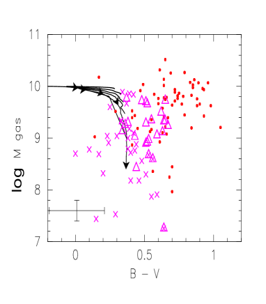
Figure 8: Comparison of predicted and observed gas masses vs $(B-V)$. Top: exponentially decreasing SFR models. Bottom: constant SFR models. Models with SFR normalisations according to $\mu_{1}=$ 0.025, 0.1, 0.3, 0.5, 0.7, and 0.9 are shown for an initial galaxy mass of $M_{\rm g}(t=0)=10^{10}$ $M_{\odot}$. Arrows on top of the $\mu_{1}=0.025$ model indicate evolution times of 1, 2, 4, 8, and 14 Gyr, respectively. Observational data as in Fig. 6

Fig. 8 demonstrates that exponentially decreasing SFR models ending at $\mu_{1}\sim 0.5$ are in good agreement with the observed hydrogen mass-to-light ratios $M_{{\rm HI}}/L_{B}$, in contrast to constant (or slowly decreasing) SFR models (expect for the bluest systems).

The conclusion that constant and slowly decreasing SFR models are inconsistent with the observed photometric and chemical properties of LSB galaxies is based on the assumption of negligible amounts of dust extinction in these systems. However, if a considerable fraction of the LSB spirals in our sample would suffer from extinctions of $E_{(B-V)}=0.1-0.25$, the $M_{{\rm HI}}/L_{B}$ ratios predicted by constant SFR models would increase by a factor $1.4-2.5$ after correction for internal extinction. In this manner, constant and slowly decreasing SFR models ending at gas fractions $\mu_{1}=0.3-0.7$ after $\sim 14$ Gyr could also explain relatively red LSB galaxies with $(B-V)\mathrel{\mathchoice{\vbox{\offinterlineskip\halign{\hfil$\displaystyle#$\hfil\cr>\cr\sim\cr}}}{\vbox{\offinterlineskip\halign{\hfil$\textstyle#$\hfil\cr>\cr\sim\cr}}}{\vbox{\offinterlineskip\halign{\hfil$\scriptstyle#$\hfil\cr>\cr\sim\cr}}}{\vbox{\offinterlineskip\halign{\hfil$\scriptscriptstyle#$\hfil\cr>\cr\sim\cr}}}}0.5$ and $M_{{\rm HI}}/L_{B}$ ratios as large as $\sim 1.5$. Even though we argued in Sect. 2 that internal extinction in LSB galaxies is unlikely to exceed $E_{(B-V)}\sim 0.1$, knowing the dust content of LSB galaxies is obviously of crucial importance in modelling their evolution.

5.2.4 Summary: the best model

To summarise, we find that exponentially decreasing SFR models ending at $\mu_{1}=0.3-0.7$ are in agreement with the colours, magnitudes, [O/H] abundances, gas contents, and mass-to-light ratios observed for LSB galaxies with $(B-V)\mathrel{\mathchoice{\vbox{\offinterlineskip\halign{\hfil$\displaystyle#$\hfil\cr>\cr\sim\cr}}}{\vbox{\offinterlineskip\halign{\hfil$\textstyle#$\hfil\cr>\cr\sim\cr}}}{\vbox{\offinterlineskip\halign{\hfil$\scriptstyle#$\hfil\cr>\cr\sim\cr}}}{\vbox{\offinterlineskip\halign{\hfil$\scriptscriptstyle#$\hfil\cr>\cr\sim\cr}}}}0.45$. Blue LSB galaxies with $(B-V)\mathrel{\mathchoice{\vbox{\offinterlineskip\halign{\hfil$\displaystyle#$\hfil\cr<\cr\sim\cr}}}{\vbox{\offinterlineskip\halign{\hfil$\textstyle#$\hfil\cr<\cr\sim\cr}}}{\vbox{\offinterlineskip\halign{\hfil$\scriptstyle#$\hfil\cr<\cr\sim\cr}}}{\vbox{\offinterlineskip\halign{\hfil$\scriptscriptstyle#$\hfil\cr<\cr\sim\cr}}}}0.45$ cannot be fitted by exponentially decreasing SFR models without an additional light contribution from a young stellar population. Alternatively, such LSB galaxies may have experienced constant SFRs, or may be much younger than 14 Gyr.

5.3 HSB/LSB: Just an extinction effect?

Since the models require an internal extinction in HSB galaxies up to $E_{(B-V)}\sim 0.5$ (corresponding to $A_{V}\sim 1.5$ mag), independent of the SFH, one could argue that extinction may be the main explanation for the difference in colour observed between LSB and HSB galaxies.

As shown in this paper the models indicate that the underlying stellar populations in LSB and HSB galaxies are still distinctly different due to differences in the chemical evolution of these systems. Therefore, extinction effects, although important, cannot be the entire explanation for the colour differences observed.

6 The effects of small star formation bursts

6.1 Luminosity contribution by HII regions in LSB galaxies

The presence of Hii regions in all the LSB galaxies in our sample suggests that recent star formation is a common phenomenon in these systems, and may thus influence the observed properties. In the previous section we found that for some LSB galaxies a simple exponential SFR was unable to explain the observed properties and that an additional “burst” of young stars was needed. Here we examine the effects of such bursts on the colours of LSB galaxies. To this end, we selected all Hii regions that could be identified by eye, either from H$\alpha$ or $R$-band CCD images, and added their total luminosity in the $I$-band. We restrict ourselves to the $I$-band data as to be least affected by extinction that may be present in or near Hii regions (McGaugh 1994). We define $\eta_{I}$ as the ratio of this Hii region integrated luminosity and the total luminosity of the corresponding LSB galaxy. As we are probably incomplete at low Hii region luminosities, this ratio gives a lower limit for the Hii region contribution to the total luminosity.

Table 4: Observed broadband contributions by Hii regions in LSB galaxies and derived SFRs

(1)	(2)	(3)	(4)	(5)	(6)	(7)	(8)	(9)
Name	#	$I$	$\eta_{\rm I}$	$(B-V)_{{\rm HII}}$	$(B-V)_{\rm gal}$	SFRcont	SFRburst	SFRtot
		[mag]		[mag]	[mag]	[M⊙ yr-1]
F561-1	15	$-$15.3	0.06	0.43	0.59	0.013	0.068	0.081
F563-1	12	$-$14.1	0.12†	0.65	0.65	0.16	1.53	1.7†
F563-V1	4	$-$13.6	0.04	0.53	0.56	0.005	0.019	0.024
F564-V3	16	$-$10.1*	0.10*	0.78	0.64	$-$	$-$	$-$
F565-V2	4	$-$12.2*	0.04*	0.72	0.53	0.017	0.055	0.072
F567-2	9	$-$14.5	0.05†	0.90†	0.67	0.029	0.12	0.15
F568-1	4	$-$14.7	0.02	0.41	0.62	0.12	0.19	0.31
F568-3	7	$-$16.1	0.07	0.53	0.55	0.06	0.27	0.33
F568-V1	11	$-$16.8	0.22	0.59	0.51	0.05	0.54	0.58
F571-5	10	$-$14.6*	0.10*	0.28	0.34	$-$	$-$	$-$
F571-V1	5	$-$13.9*	0.04*	0.40	0.53	0.033	0.11	0.14
F574-2	4	$-$14.0*	0.03*	0.46	0.63	0.012	0.029	0.041
F577-V1	14	$-$16.3*	0.19*	0.39	0.38	$-$	$-$	$-$
U128	17	$-$16.2	0.06	0.55	0.51	0.14	0.68	0.82
U628	26	$-$17.8	0.17	0.55	0.56	$-$	$-$	$-$
U1230	24	$-$16.2	0.08	0.43	0.52	0.05	0.34	0.39

* values refer to $R$ band magnitudes instead of $I$-band
† uncertain due to contamination by fore- or background objects
— $\mu_{\rm rot}$ not determined

In columns (1) and (2) of Table 4, we list the LSB galaxy identification and number of Hii regions selected. The number of Hii regions identified within individual LSB galaxy ranges from a few to $\sim 25$. For the ensemble of Hii regions in each LSB galaxy, we tabulate the absolute $I$ magnitudes as well as the corresponding ratios $\eta_{I}$ of the Hii region integrated luminosity and total LSB galaxy luminosity, in columns (3) and (4). Mean ($B-V$) colours for the Hii regions and for the LSB galaxy as a whole are given in columns (5) and (6), respectively.

For most of the LSB galaxies in our sample, the contribution of the Hii regions to the total light emitted by LSB galaxies does not exceed $\eta_{I}=0.05-0.1$. However, as Hii regions are likely to contain an increased amount of dust (McGaugh 1994) the actual contributions may be higher by a factor of $\sim 2$ in $I$. Thus, the values of $\eta_{I}$ provide lower limits to the actual luminosity contributions of the Hii regions. For some LSB galaxies, e.g. F568-V1 and F577-V1, the Hii region contribution is found to be as high as $\eta_{I}=0.2$. These systems contain a only modest number of Hii regions so that their Hii regions on average may be larger and/or brighter than those present in several other LSB galaxies.

Figure 10 shows the resulting Hii region contributions $\eta_{I}$ for the SFR models discussed in Sect. 4. If we assume a maximum age $\tau_{\rm HII}=5$ Myr for the Hii regions observed, then this implies that stars more massive than $\sim 25$ $M_{\odot}$ are associated with these regions, according to the stellar evolution tracks from the Geneva group (see below).

Corrections for dust extinction within the Hii regions and LSB galaxy as a whole, respectively, will shift the observations in the directions as indicated in Fig. 10 (assuming a mean Galactic extinction curve). From the $I$ band observations we can conclude that the values of $\eta_{I}$ predicted by smoothly varying SFR models are systematically too low for most of the LSB galaxies in our sample.

This is true in particular for F568-V1, F577-V1, and U628 for which values of $\eta_{I,R}\mathrel{\mathchoice{\vbox{\offinterlineskip\halign{\hfil$\displaystyle#$\hfil\cr>\cr\sim\cr}}}{\vbox{\offinterlineskip\halign{\hfil$\textstyle#$\hfil\cr>\cr\sim\cr}}}{\vbox{\offinterlineskip\halign{\hfil$\scriptstyle#$\hfil\cr>\cr\sim\cr}}}{\vbox{\offinterlineskip\halign{\hfil$\scriptscriptstyle#$\hfil\cr>\cr\sim\cr}}}}0.2-0.25$ suggest that star formation has been recently enhanced by factors $\sim 5-10$ relative to the SFRs predicted by exponentially decreasing or constant SFR models.

6.2 Effects of small amplitude star formation bursts

We investigate whether the observed values of $\eta_{I}\sim 0.25$ in the $I$ band, as observed for several LSB galaxies discussed above, can be explained by small-amplitude bursts of star formation.

We assume a Gaussian star formation burst profile with a given amplitude $A_{b}$ and dispersion $\sigma$. We follow its evolution during 1 Gyr with a time resolution of $\sim 0.1$ Myr at time of burst maximum and of $\sim 2$ Myr at roughly 5$\sigma$ from burst maximum. We superimpose the star formation burst on an exponential SFR model, as discussed in Sect. 5.1.

We initially assume a galactic evolution time at burst maximum of $t_{\rm b}=13$ Gyr, burst maximum amplitude $A_{\rm b}=8$ $M_{\odot}$  yr^-1, burst duration $\Delta t_{\rm b}=5$ Myr, maximum Hii region lifetime $\tau_{\rm H{II}}=5$ Myr, and an initial galaxy mass of $10^{10}$ $M_{\odot}$. For simplicity, we neglect any influence of the burst on the chemical evolution of the model galaxy.

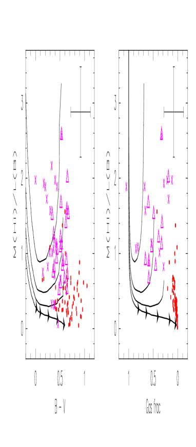
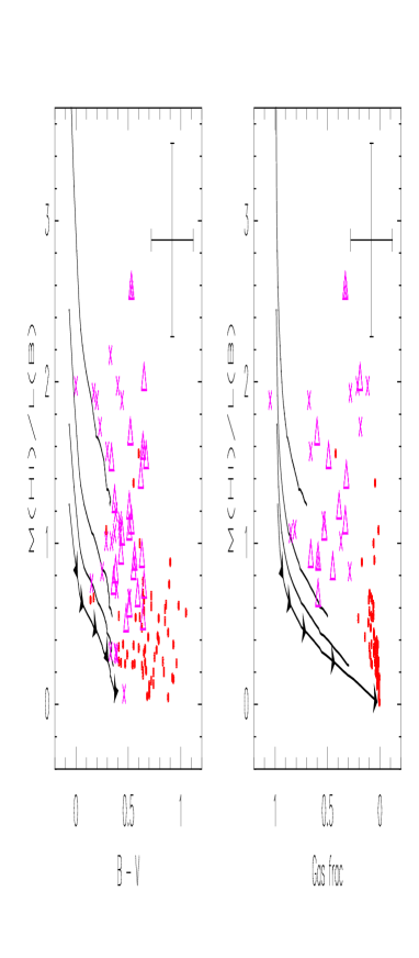
Figure 9: Evolution of $M_{{\rm HI}}/L_{B}$ vs $(B-V)$ (left) and $M_{{\rm HI}}/L_{B}$ vs $\mu_{1}$ (right). Top panels: exponentially decreasing SFR models, bottom panels: constant SFR models. From bottom to top, curves are shown for models ending at increasing gas fractions $\mu_{1}=$ 0.1, 0.3, 0.5, and 0.7, respectively. Arrows on top of the $\mu_{1}=0.1$ model indicate evolution times of 1, 2, 4, 8, and 14 Gyr, respectively. Observational data as in Fig. 8

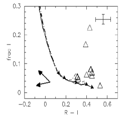
Figure 10: Evolution of the Hii region integrated luminosity contribution for different SFR models ending at $\mu_{1}=0.1$. Shown is the ratio of Hii region integrated and total luminosity in the $I$ band $\eta_{I}$ vs $(R-I)$. For the exponentially decreasing SFR model, solid triangles indicate evolution times of 1, 2, 4, 8, and 14 Gyr, respectively. Observational data on LSB galaxies is shown as open triangles. Typical errors in the data (upper right) and directions to which the data would shift after corrections for extinction (bottom left) are indicated. Top and bottom arrows indicate corrections for extinction within the Hii regions and the LSB galaxy for $E_{R-I}=0.1$, respectively

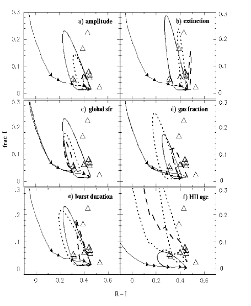
Figure 11: Impact of small amplitude bursts on the evolution of the Hii region integrated luminosity contribution in the $I$-band $\eta_{I}$ vs $(R-I)$. Unless stated otherwise, we plot the exponentially decreasing SFR + burst model assuming $A_{\rm b}=8$ $M_{\odot}$  yr^-1, $\Delta t_{\rm b}=5$ Myr, $\tau_{{\rm HII}}=5$ Myr, and $E_{{B}-{V}}=0$ mag. a) effect of varying burst amplitude: $A_{\rm b}=8$ (solid curve), 4 (dotted), and 1.6 (dashed) $M_{\odot}$  yr^-1; b) effect of mean extinction within Hii regions: $E_{{B}-{V}}$ = 0.25 (solid curve), 0.5 (dotted), and 1 (dashed); c) effect of global star formation history: exponentially decreasing SFR (solid curve), constant (dotted), and linearly increasing (dashed); d) effect of actual gas-to-total mass ratio: $\mu_{1}=0.1$ (dashed curve), 0.5 (solid), and 0.7 (dotted); e) effect of burst duration: $\Delta t_{\rm b}$ = 1 (dashed curve), 5 (solid), and 10 (dotted) Myr; f) effect of Hii region age: $\tau_{{\rm HII}}$ = 2 (solid curve), 10 (dotted), and 50 (dashed; no burst shown) Myr. Symbols have the same meaning as in Fig. 10.

We show the result in Fig. 11a. At $t=t_{b}=13$ Gyr the contribution by young stars increases rapidly. Simultaneously, the $(R-I)$ colours become significantly bluer. After burst maximum, the contribution by young stars decreases again and galaxy colours start to redden until the effect of the burst becomes negligible and colours and magnitudes evolve as prior to the burst.

In this manner, a characteristic burst loop is completed as shown in Fig. 11a. The shape of this loop is determined by: i) the burst amplitude, ii) the extinction within the Hii regions, iii) the contribution by the old stellar population to the integrated galaxy light, iv) the duration (and profile) of the burst, v) the maximum time during which young stars produced by the Hii regions can still be distinguished from the surrounding field population.

Burst amplitude and IMF: Fig. 11a demonstrates that values of $\eta_{I}\sim 0.25$ can be well explained by bursts with amplitude $A_{\rm b}=8$ $M_{\odot}$yr^-1 superimposed on an exponentially decreasing SFR model ending at $\mu_{1}=0.1$. Decreasing the burst amplitude by factors 2.5 and 5, respectively, results in the smaller loops shown in Fig. 11a. The actual burst amplitude required to explain the observations depends on many quantities as described below

Dust extinction: Fig. 11b illustrates the effect of dust extinction on $\eta_{I}$ and $(R-I)$. A selective extinction of $E_{{B}-{V}}=(0.25,0.5,1)$ mag for the Hii regions results in a reduction $\eta_{I}$ by a factor (1.6, 2.5, 6.5) and a reddening $E_{R-I}=$ (0.14, 0.27, 0.56) mag, assuming a Galactic extinction curve. For values of $E_{{B}-{V}}\mathrel{\mathchoice{\vbox{\offinterlineskip\halign{\hfil$\displaystyle#$\hfil\cr>\cr\sim\cr}}}{\vbox{\offinterlineskip\halign{\hfil$\textstyle#$\hfil\cr>\cr\sim\cr}}}{\vbox{\offinterlineskip\halign{\hfil$\scriptstyle#$\hfil\cr>\cr\sim\cr}}}{\vbox{\offinterlineskip\halign{\hfil$\scriptscriptstyle#$\hfil\cr>\cr\sim\cr}}}}0.5$ mag, we find that the bluing effect on $(R-I)$ by young massive stars formed during the burst is neutralised almost entirely by extinction. For intense bursts reddening of the galaxy colours may even occur. If variations in the mean extinction of the ensembles of Hii regions among LSB galaxies are small (e.g. less than a factor two), it is difficult to see how extinction alone can provide an adequate explanation for the large variations observed in $\eta_{I}$.

Global star formation history: From Fig. 11c it is clear that the burst effect on the galaxy magnitudes and colours increases when the contribution by the old stellar population is decreased. Thus, colours and magnitudes are less affected by bursts imposed on constant or even increasing SFRs compared to those imposed on exponentially decreasing SFR models: the smaller loop sizes just reflect that the mean age of the underlying stellar population is relatively low.

Current gas fraction: Fig. 11d demonstrates how the present-day gas fraction $\mu_{1}$ affects the effect of the burst. The luminosity contribution by the old stellar population decreases for increasing values of $\mu_{1}$, and thus, as discussed above, we find that the effect of a star formation burst for galaxies with $\mu_{1}=0.9$ (i.e. unevolved systems) is as large as that of a ten times stronger burst for $\mu_{1}=0.1$ (i.e. highly evolved systems). Thus, the burst amplitude required to explain the observations strongly depends on the present-day gas-to-total mass-ratio.

Burst duration: Fig. 11e shows that the duration of the burst affects the impact of the burst as well. For $\Delta t_{\rm b}=1$, 5, and 10 Myr, the variation in $\eta_{I}$ is $\sim 0.25$ while the resulting galaxy $(R-I)$ colours become bluer. Burst durations in excess of $\Delta t_{\rm b}\sim 5$ Myr are unlikely since this would require dust extinctions $E_{(B-V)}\mathrel{\mathchoice{\vbox{\offinterlineskip\halign{\hfil$\displaystyle#$\hfil\cr>\cr\sim\cr}}}{\vbox{\offinterlineskip\halign{\hfil$\textstyle#$\hfil\cr>\cr\sim\cr}}}{\vbox{\offinterlineskip\halign{\hfil$\scriptstyle#$\hfil\cr>\cr\sim\cr}}}{\vbox{\offinterlineskip\halign{\hfil$\scriptscriptstyle#$\hfil\cr>\cr\sim\cr}}}}1$ mag in order to provide agreement with the observed $(R-I)$ colours (cf. Fig. 11b). Such large extinction in Hii regions are probably excluded by the observations (e.g. McGaugh 1994). Thus, relatively narrow burst profiles are needed to explain extreme values $\eta_{I}\sim 0.2$ (as in F568-V1; cf. Table 4).

Maximum age of Hii regions: Fig. 11f shows that when the maximum lifetime of the Hii regions is increased from $\tau_{{\rm HII}}=5$ to 50 Myr, partial agreement with the observations can be achieved without invoking star formation bursts. We note that the resulting Hii region contributions do not increase linearly with $\tau_{{\rm HII}}$ as short lived massive stars dominate the luminosity contribution of all stars formed during the past $\tau_{{\rm HII}}$ yr.

Values of $\tau_{{\rm HII}}\mathrel{\mathchoice{\vbox{\offinterlineskip\halign{\hfil$\displaystyle#$\hfil\cr>\cr\sim\cr}}}{\vbox{\offinterlineskip\halign{\hfil$\textstyle#$\hfil\cr>\cr\sim\cr}}}{\vbox{\offinterlineskip\halign{\hfil$\scriptstyle#$\hfil\cr>\cr\sim\cr}}}{\vbox{\offinterlineskip\halign{\hfil$\scriptscriptstyle#$\hfil\cr>\cr\sim\cr}}}}50$ Myr would mean that stars down to masses of $m_{\rm ion}\mathrel{\mathchoice{\vbox{\offinterlineskip\halign{\hfil$\displaystyle#$\hfil\cr<\cr\sim\cr}}}{\vbox{\offinterlineskip\halign{\hfil$\textstyle#$\hfil\cr<\cr\sim\cr}}}{\vbox{\offinterlineskip\halign{\hfil$\scriptstyle#$\hfil\cr<\cr\sim\cr}}}{\vbox{\offinterlineskip\halign{\hfil$\scriptscriptstyle#$\hfil\cr<\cr\sim\cr}}}}7$ $M_{\odot}$ would contribute to the Hii regions identified (e.g. Schaerer et al. 1993; $Z=0.001$). Observational estimates for $m_{\rm ion}$ are usually in the range $10-15$ $M_{\odot}$ (Wilcots 1994; García-Vargas 1995) and correspond to $\tau_{{\rm HII}}\mathrel{\mathchoice{\vbox{\offinterlineskip\halign{\hfil$\displaystyle#$\hfil\cr>\cr\sim\cr}}}{\vbox{\offinterlineskip\halign{\hfil$\textstyle#$\hfil\cr>\cr\sim\cr}}}{\vbox{\offinterlineskip\halign{\hfil$\scriptstyle#$\hfil\cr>\cr\sim\cr}}}{\vbox{\offinterlineskip\halign{\hfil$\scriptscriptstyle#$\hfil\cr>\cr\sim\cr}}}}15$ Myr. Even though these values would imply that our adopted value of $\tau_{{\rm HII}}=5$ Myr is too low, this excludes extreme values of $\tau_{{\rm HII}}=200$ Myr which would be required to explain the observed range in $\eta_{I}$ exclusively in terms of variations in $\tau_{{\rm HII}}$ and/or $m_{\rm ion}$. Therefore, variations in $\tau_{{\rm HII}}$ (or equivalently $m_{\rm ion}$) and/or extinction may provide an explanation only for part of the variations in the Hii region integrated luminosity contributions observed among LSB galaxies.

Table 5: Maximum changes induced on galaxy magnitudes and colours for $M_{g}=10^{10}\ M_{\odot}$
by a 5 Myr starburst

Model	$A_{\rm b}$	$\Delta B$	$\Delta I$	$\Delta(B-V)$	$\Delta(R-I)$	Notes
	[$M_{\odot}$  yr-1]	[mag]	[mag]	[mag]	[mag]
A1+burst	0.8	$-$0.34	$-$0.14	$-$0.18	$-$0.04	SFR1 = 0.17 $M_{\odot}$yr-1
”	1.6	$-$0.58	$-$0.30	$-$0.28	$-$0.10
”	3.0	$-$1.05	$-$0.42	$-$0.43	$-$0.17	*
”	8.0	$-$1.72	$-$0.53	$-$0.56	$-$0.26	*
B1+burst	0.8	$-$0.14	$-$0.06	$-$0.08	$-$0.02	SFR1 = 0.89 $M_{\odot}$yr-1
”	1.6	$-$0.32	$-$0.21	$-$0.11	$-$0.07
”	3.0	$-$0.56	$-$0.32	$-$0.21	$-$0.11	*
”	8.0	$-$0.94	$-$0.41	$-$0.33	$-$0.14	*

* $E_{(B-V)}\mathrel{\mathchoice{\vbox{\offinterlineskip\halign{\hfil$\displaystyle#$\hfil\cr>\cr\sim\cr}}}{\vbox{\offinterlineskip\halign{\hfil$\textstyle#$\hfil\cr>\cr\sim\cr}}}{\vbox{\offinterlineskip\halign{\hfil$\scriptstyle#$\hfil\cr>\cr\sim\cr}}}{\vbox{\offinterlineskip\halign{\hfil$\scriptscriptstyle#$\hfil\cr>\cr\sim\cr}}}}0.3$ mag in Hii regions is required to provide agreement with observations

In conclusion, the observations suggest that small amplitude, short bursts of star formation are important in at least several of the LSB galaxies for which accurate photometry data is available. Such recent episodes of enhanced star formation may play an important role in affecting the colours of the blue LSB galaxies.

6.3 Quantitative effect of small amplitude bursts on galaxy colours and magnitudes

Table 5 lists the effect of a 5 Myr star formation burst on the galaxy integrated magnitudes and colours for various burst amplitudes. For an exponentially decreasing SFR (model A1 in Table 3; assuming $M_{\rm g}(0)=10^{10}$ $M_{\odot}$, $\mu_{1}=0.1$, Salpeter IMF), we find that a burst with amplitude $A_{\rm b}=0.8$ $M_{\odot}$  yr^-1 results in maximum colour variations $\Delta(B-V)$ and $\Delta(R-I)$ of $-0.18$ and $-0.04$ mag, respectively. The effect of increasing the burst amplitude by a factor 10 to $A_{\rm b}=8$ $M_{\odot}$  yr^-1 results in corresponding shifts of $-0.56$ and $-0.26$ mag, respectively. This effect is similar to that when the initial galaxy mass is reduced by a factor ten while leaving the burst amplitude unaltered (i.e. for. $M_{\rm g}(0)=10^{9}$ $M_{\odot}$ and $A_{\rm b}=0.8$ $M_{\odot}$  yr^-1).

For bursts superimposed on exponentially decreasing SFRs models ending at $\mu_{1}=0.1$, the colour and magnitude shifts predicted are consistent with the observations in case of burst amplitudes $A_{\rm b}\mathrel{\mathchoice{\vbox{\offinterlineskip\halign{\hfil$\displaystyle#$\hfil\cr<\cr\sim\cr}}}{\vbox{\offinterlineskip\halign{\hfil$\textstyle#$\hfil\cr<\cr\sim\cr}}}{\vbox{\offinterlineskip\halign{\hfil$\scriptstyle#$\hfil\cr<\cr\sim\cr}}}{\vbox{\offinterlineskip\halign{\hfil$\scriptscriptstyle#$\hfil\cr<\cr\sim\cr}}}}3$ $M_{\odot}$  yr^-1, assuming a typical extinction of $E_{(B-V)}=0.3$ mag in the Hii regions. In fact, the effect of the burst is determined mainly by the total luminosity of the young stellar populations formed according to the continuous SFR during the last Gyr or so. Since the amplitude of the SFR scales with $(1-\mu_{1})$ for models ending at different gas fractions $\mu_{1}$ the impact of the burst for models ending at $\mu_{1}=0.5$ is about twice that given in Table 5. Similarly, for models ending at $\mu_{1}\mathrel{\mathchoice{\vbox{\offinterlineskip\halign{\hfil$\displaystyle#$\hfil\cr>\cr\sim\cr}}}{\vbox{\offinterlineskip\halign{\hfil$\textstyle#$\hfil\cr>\cr\sim\cr}}}{\vbox{\offinterlineskip\halign{\hfil$\scriptstyle#$\hfil\cr>\cr\sim\cr}}}{\vbox{\offinterlineskip\halign{\hfil$\scriptscriptstyle#$\hfil\cr>\cr\sim\cr}}}}0.9$, the burst effect becomes roughly ten times stronger compared to the $\mu_{1}=0.1$ case (cf. Fig. 11). The effect of the burst is substantially reduced when going from exponentially decreasing to constant SFRs (cf. Table 5).

Table 6: Model SFR and gas fractions

(1)	(2)
$\mu_{1}$	$A$
	$(M_{\odot}{\rm yr}^{-1})$
0.1	0.18
0.3	0.13
0.5	0.09
0.7	0.06
0.9	0.02

Table 7: Observational estimates of present-day SFRs [$M_{\odot}$yr^-1] in LSB galaxies^∗

(1)	(2)	(3)	(4)	(5)	(6)	(7)	(8)	(9)	(10)	(11)	(12)
Name	Dist.	$m_{I}$	R${}^{27}_{I}$	RHI	$\mu_{I}$	MHI	$\langle\sigma_{\rm HI}\rangle$	SFR${}^{\rm fix}_{1}$	SFR1	SFRcont	SFRtot
	[Mpc]	[mag]	[kpc]	[kpc]	[mag arcsec-2]	[$M_{\odot}$]	[$M_{\odot}$pc-2]	[$M_{\odot}$yr-1]
F561-1	47	14.7	6.6	7.6	23.2	8.91	4.5	0.05	0.09	0.013	0.081
F563-1	34	16.1	10.2	16.3	26.4	9.19	1.0	(0.03)	(0.02)	0.16	1.7†
F563-V1	38	15.8	4.6	4.8	24.0	8.48	4.2	0.02	0.03	0.005	0.024
F567-2	56	15.9	8.4	10.6	24.6	9.09	3.5	0.04	0.06	0.029	0.15
F568-1	64	15.0	9.6	11.5	23.7	9.35	5.4	0.08	0.18	0.12	0.31
F568-3	58	14.7	8.7	11.4	23.3	9.20	3.9	0.09	0.14	0.06	0.33
F568-V1	60	15.7	8.4	10.7	24.3	9.14	3.8	0.05	0.07	0.05	0.58
U128	48	13.5	18.2	21.4	24.1	9.55	(2.0)	(0.16)	(0.21)	0.14	0.82
U1230	40	14.3	12.0	18.8	24.5	9.51	(4.3)	(0.11)	(0.15)	0.05	0.39

Notes: ^∗ theoretical values in columns (11) and (12) repeat those in columns (9) and (11) from Table 4; † probably contaminated by field galaxy. Values between parentheses are uncertain.

7 Present-day star formation rates in LSB galaxies

7.1 Theoretical star formation rates

7.1.1 Continuous SFR

Theoretical SFRs can be derived from the models discussed in the previous section (exponentially decreasing SFR, Salpeter IMF), using:

$${\rm SFR}^{\rm cont}\approx A(\mu_{1})\frac{M^{\rm tot}}{10^{10}}\>\ \ {M}_{\odot}\,{\rm yr}^{-1}$$ (3)

where $A(\mu_{\rm 1})$ is the model SFR amplitude required to end at a gas fraction $\mu_{1}$ at a galactic evolution time of 14 Gyr (assuming an initial mass of $10^{10}$ $M_{\odot}$) and $M^{\rm tot}$ the total galaxy mass as obtained from $M_{{\rm HI}}$ and $\mu_{\rm 1}$.

We list the required values for $A$ to have the models end at certain values of $\mu_{1}$ in Table 6. Using these values we find that LSB galaxies show present-day SFRs (without bursts) between $0.01\mathrel{\mathchoice{\vbox{\offinterlineskip\halign{\hfil$\displaystyle#$\hfil\cr<\cr\sim\cr}}}{\vbox{\offinterlineskip\halign{\hfil$\textstyle#$\hfil\cr<\cr\sim\cr}}}{\vbox{\offinterlineskip\halign{\hfil$\scriptstyle#$\hfil\cr<\cr\sim\cr}}}{\vbox{\offinterlineskip\halign{\hfil$\scriptscriptstyle#$\hfil\cr<\cr\sim\cr}}}}{\rm SFR}^{\rm cont}\mathrel{\mathchoice{\vbox{\offinterlineskip\halign{\hfil$\displaystyle#$\hfil\cr<\cr\sim\cr}}}{\vbox{\offinterlineskip\halign{\hfil$\textstyle#$\hfil\cr<\cr\sim\cr}}}{\vbox{\offinterlineskip\halign{\hfil$\scriptstyle#$\hfil\cr<\cr\sim\cr}}}{\vbox{\offinterlineskip\halign{\hfil$\scriptscriptstyle#$\hfil\cr<\cr\sim\cr}}}}0.15$$M_{\odot}$yr^-1. For a typical LSB galaxy (i.e. $M^{\rm tot}=10^{10}$ $M_{\odot}$, $\mu_{1}=0.5$) we estimate SFR${}^{\rm cont}=0.1$ $M_{\odot}$yr^-1.

7.1.2 Burst SFR

As we discussed in Sect. 6, the effect of a starburst on the galaxy integrated magnitudes and colours depends on many quantities. However, assuming a modest Hii region extinction of $E_{(B-V)}=0.25$ mag and lifetime $\tau_{{\rm HII}}=20$ Myr, crude estimates for the maximum burst amplitude can be derived from:

$${\rm SFR}^{\rm burst}\>\approx 20\eta_{\rm I}\>\frac{M_{{\rm HI}}}{10^{10}}\>\left(\frac{1}{\mu_{\rm rot}}-1\right)\\ \ {M}_{\odot}{\rm yr}^{-1}$$ (4)

We find that $I$-band contributions of $\eta_{\rm I}=0.2$ are best explained by a 5 Myr burst with amplitude SFR${}^{\rm burst}=0.8$ $M_{\odot}$yr^-1, assuming present-day values of $M_{{\rm HI}}=2\cdot 10^{9}$ $M_{\odot}$ and $\mu_{\rm rot}=0.5$.

Theoretical estimates for the total current SFRs in LSB galaxies are found from ${\rm SFR}^{\rm tot}={\rm SFR}^{\rm cont}+{\rm SFR}^{\rm burst}$ and are listed in the last two columns of Table 7. Present-day SFRs for LSB galaxies experiencing small amplitude bursts range from SFR${}^{\rm tot}\sim 0.02$ to 0.8 $M_{\odot}$  yr^-1.

7.2 Empirical star formation rates

We have also derived current SFRs for LSB galaxies using the empirical method presented by Ryder & Dopita (1994; hereafter RD) based on CCD surface photometry of galactic disks. These authors found a relationship between the local H$\alpha$ and $I$-band surface brightness in the disks of a sample of 34 of southern spiral galaxies. From this relation, RD derived a constraint on the present-day SFR integrated over the entire stellar mass spectrum as: $$\log{\rm SFR_{1}}=-0.26\mu_{I}+0.92\log\sigma_{\rm HI}+5.3$$ $$\hfill{M}_{\odot}{\rm pc}^{-2}{\rm Gyr}^{-1}\ \ \ \$$ (5) where $\mu_{I}$ is the $I$-band surface brightness and $\sigma_{\rm HI}$ is the global mean Hi surface density [$M_{\odot}$pc^-2] within the star-forming disk. The relation between SFR₁ and $\mu_{I}$ is normalised by a term related to the mean surface density $\sigma_{\rm HI}$ and by a constant which is partly related to the conversion of the massive star formation rate to total SFR depending on the adopted IMF (cf. Kennicutt 1983). It is unclear from the RD sample whether the relation is valid also for the lowest (stellar) $I$-band surface densities that are observed among LSB galaxies. However, since this relation holds over a wide range in surface brightness and massive star formation in the disks of spirals it appears rather insensitive to galactic dynamics, extinction, and molecular gas content (RD), we expect this relation to be valid also in case of LSB galaxies. At the faintest surface brightnesses (i.e. $\mu_{I}\mathrel{\mathchoice{\vbox{\offinterlineskip\halign{\hfil$\displaystyle#$\hfil\cr>\cr\sim\cr}}}{\vbox{\offinterlineskip\halign{\hfil$\textstyle#$\hfil\cr>\cr\sim\cr}}}{\vbox{\offinterlineskip\halign{\hfil$\scriptstyle#$\hfil\cr>\cr\sim\cr}}}{\vbox{\offinterlineskip\halign{\hfil$\scriptscriptstyle#$\hfil\cr>\cr\sim\cr}}}}25.6$ mag arcsec^-2), the relation may be flattening off although the effects of sky subtraction and small number statistics leave this open to question. If flattening indeed occurs, Eq. (5) provides lower limits to the actual SFRs in LSB galaxies.

Using Eq. (3), we estimate global present-day SFRs for all LSB galaxies in our sample with measured $I$-band magnitudes and related data. For these LSB galaxies we list the distance, apparent $I$-band magnitude, and radius $R_{27}$ of the 27 mag arcsec^-2 $B$-band isophote, in columns (2) to (4) in Table 7. This radius corresponds to the optical edge of the LSB galaxy and is more representative for the radius within which the old disk stellar population in LSB galaxies is contained than is $R_{25}$ as used by RD for HSB galaxies. Accordingly, we define an effective I band surface brightness as:

$$\mu_{I}^{\rm eff}=m_{I}+2.5\log(\pi R_{27}^{2})$$ (6)

and use this in Eq. (5). We tabulate the outermost radius of the measured Hi rotation curve $R_{{\rm HI}}$, effective $I$ band surface brightness $\mu_{I}^{\rm eff}$, total Hi mass derived within $R_{{\rm HI}}$, and the mean global surface Hi density $\sigma_{{\rm HI}}$ in columns (5) to (8), respectively. For a consistent comparison between effective surface brightness and global Hi surface density, one ought to measure them out to the same radius (e.g. $R_{27}$). However, since $M_{\rm HI}$ has been measured within $R_{{\rm HI}}$, we expect the former values to be more representative of the average Hi surface density in the star forming part of the disk. The mean global Hi surface densities $\sigma_{\rm HI}$ derived using $R_{\rm HI}$ vary between 2 and 5.5 $M_{\odot}$pc^-2 and are substantially smaller (i.e. by $20-60$ %) than those derived using $R_{27}$ instead.

The empirically derived mean present-day SFRs for the LSB galaxies from our sample range from about SFR${}_{1}=0.02$ to $\sim 0.2$ $M_{\odot}$yr^-1 (cf. column 10 of Table 7). Errors arising from the Hi normalisation are estimated to be within a factor of two. This is illustrated when the same SFRs are derived assuming a fixed Hi surface density of 2 $M_{\odot}$pc^-2 for all LSB galaxies (cf. SFR${}_{1}^{\rm fix}$ in Table 7).

The empirically derived current SFRs in LSB galaxies are in good agreement with the theoretically derived SFRs ranging from SFR${}^{\rm cont}\sim 0.01$ to 0.15 $M_{\odot}$yr^-1 (cf. Table 7). As discussed before, the theoretically derived present-day SFRs of individual LSB galaxies lie probably between SFR^cont and SFR^tot where the latter values include the contribution of small amplitude bursts (SFR${}^{\rm tot}=\$SFR${}^{\rm cont}+$SFR^burst). In several cases, the values of SFR^tot are considerably larger than the empirical values which suggests that the burst contribution is overestimated by the models and/or that the SFRs derived empirically do not trace well local enhancements of star formation at the faint surface brightnesses of LSB galaxies.

The present-day SFRs in LSB galaxies are thus found to be considerably below the $\sim 5-10$ $M_{\odot}$yr^-1 derived for their HSB counterparts (e.g. Kennicutt 1992 and references therein) but significantly larger than the $\sim 0.001$ $M_{\odot}$yr^-1 observed typically in dwarf irregular galaxies (e.g. Hunter & Gallagher 1986).

8 Discussion

In the previous sections we have focussed on the difference between HSB galaxies and the type of LSB galaxies we have in our sample. As noted in the introduction (and also shown in Fig. 1) HSB and LSB galaxies, however, do not form separate groups. In fact there is a broad range of galaxy properties and the purpose of the discussion is to clarify what role the star formation history plays in determining the final character of a galaxy.

In general, there appears a trend along the Hubble sequence from rapidly decaying SFRs for early type galaxies to constant or even increasing SFRs for dwarf irregular galaxies (see e.g. reviews by Sandage 1986; Kennicutt 1992). On average, the observed trend corresponds to a decrease of the ratio of mean past to present SFR along the Hubble sequence. Most of the LSB galaxies in our sample belong to the group of late-type galaxies for which exponentially decreasing SFR models are in good agreement with the observations. The remaining LSB galaxies, for which slowly decreasing or constant (sporadic) SFR models are more appropriate, belong to a group of galaxies with properties intermediate to those of disk galaxies with weak or absent spiral arms and Sm/Im galaxies. Thus, in general LSB galaxies comply well with the observed trend of SFR variation with Hubble type.

The “burst” scenario discussed in section 6 indicates that current star formation in virtually all the LSB galaxies in our sample is local both in time and space and suggests that sporadic star formation has been a continuous process from the time star formation started in the disks of LSB galaxies.

The low star formation rates of $\sim$0.1 $M_{\odot}$yr^-1 derived for LSB galaxies as well as the local nature of the star formation in these systems are consistent with the idea of a critical threshold for the onset of global star formation in disk galaxies (e.g. Skillman 1987; Kennicutt 1989; Davies 1990).

Even though LSB galaxies contain large amounts of gas, only very limited amounts participate in the process of star formation. If we assume that LSB galaxies maintain their current star formation rate of $\sim$0.1 $M_{\odot}$yr^-1, their typical present-day amount of gas $\sim$ M_g = 2.5 10⁹ $M_{\odot}$ will be consumed within $\tau_{\rm gas}\sim$30 Gyr (for a recycled fraction of 25%). Such gas consumption times for LSB galaxies are much larger than a Hubble time (e.g. Romanishin 1980). For comparison, $\tau_{\rm gas}\sim 2-4$ Gyr in HSB galaxies, assuming typically M${}_{\rm g}\sim 10^{10}$ $M_{\odot}$ and SFR${}_{1}\sim 5$ $M_{\odot}$yr^-1, which implies that HSB galaxies will run out of gas soon (see Kennicutt 1992).

The presence of an old stellar population in many late-type LSB galaxies as indicated by their optical colours (e.g. vdH93; dB95) and as confirmed by the results from the modelling suggests that LSB galaxies roughly follow the same evolutionary history as HSB galaxies, but at a much lower rate.

The models suggest that very slowly decreasing star formation rates with $e$-folding times much larger than $\sim$ 5 Gyr probably can be ruled out for the majority of the LSB galaxies examined here. The observed colours are too blue, provided extinction is indeed negligible. This result is insensitive to the possible occurrence of infall or accretion of gas. Similarly the models indicate that the dominant stellar population in galaxies with $(B-V)\geq 0.5$ mag cannot be as young as 10 or 5 Gyr (cf. Fig. 5). In contrast the models can not rule out a dominant luminosity contribution by stellar populations significantly younger than 5 – 10 Gyr for LSB galaxies with $(B-V)\approx 0.4$.

First this indicates that the mean age of the stellar population in most LSB and HSB galaxies is similar even though the disks of LSB galaxies are in a relative early evolutionary stage. Although we have not explored an entire range of star formation e-folding times, values much below or in excess of $\sim$ 5 Gyr are not very likely. Smaller values would increase the colour contribution from the underlying older stellar population and hence produce redder colours than observed, while much larger values correspond to slowly decreasing or almost constant star formation rates implying a relatively larger contribution of the younger stellar population.

Secondly, the combined effect of extinction and metallicity on galaxy colours is sufficient to explain the colour differences observed between LSB galaxies and HSB galaxies. Since the amount of extinction depends strongly on the dust content, which in turn is coupled to the heavy element abundances in the ISM (see Sect. 2), metallicity probably is the main quantity determining the colour differences observed between LSB and HSB galaxies. In this manner the much lower rate of star formation in LSB galaxies, implying lower metallicities and dust contents, indirectly determines the blue colours of LSB galaxies compared to HSB galaxies.

9 Summary

We have examined the star formation histories of LSB galaxies using models which take into account both the photometric and the chemical evolution of the galaxies. For the majority of the LSB galaxies in our sample, observed $UBVRI$ magnitudes, [O/H] abundances, gas masses and fractions, and Hi mass-to-light ratios are best explained by an exponentially decreasing global SFR ending at a present-day gas-to-total mass-ratio of $\mu_{1}\sim 0.5$. When small amplitude bursts are involved to decrease the predicted $M_{\rm g}/L$ ratios, models ending at $\mu_{1}\approx 0.7$ may also apply. In addition to exponentially decreasing SFR models, $\sim 15\%$ of the LSB galaxies require modest amounts of internal extinction $E_{(B-V)}\mathrel{\mathchoice{\vbox{\offinterlineskip\halign{\hfil$\displaystyle#$\hfil\cr<\cr\sim\cr}}}{\vbox{\offinterlineskip\halign{\hfil$\textstyle#$\hfil\cr<\cr\sim\cr}}}{\vbox{\offinterlineskip\halign{\hfil$\scriptstyle#$\hfil\cr<\cr\sim\cr}}}{\vbox{\offinterlineskip\halign{\hfil$\scriptscriptstyle#$\hfil\cr<\cr\sim\cr}}}}0.1$ mag to explain the relatively red colours of $(B-V)\sim 0.6$ of these systems.

A substantial fraction ($\sim 35\%$) of the LSB galaxies in our sample have colours $(B-V)\mathrel{\mathchoice{\vbox{\offinterlineskip\halign{\hfil$\displaystyle#$\hfil\cr<\cr\sim\cr}}}{\vbox{\offinterlineskip\halign{\hfil$\textstyle#$\hfil\cr<\cr\sim\cr}}}{\vbox{\offinterlineskip\halign{\hfil$\scriptstyle#$\hfil\cr<\cr\sim\cr}}}{\vbox{\offinterlineskip\halign{\hfil$\scriptscriptstyle#$\hfil\cr<\cr\sim\cr}}}}0.45$ mag and exhibit properties similar to those resulting from exponentially decreasing SFR models at evolution times of $\sim 5-10$ Gyr. Alternatively, recent episodes of enhanced star formation superimposed on exponentially decreasing SFR models may provide an adequate explanation for the colours of these systems (see Sect. 6). Recent star formation is observed, at least at low levels, in essentially all the LSB galaxies in our sample. Hence, it seems justified to assume that the disks in LSB galaxies experienced continuous (i.e. frequent small amplitude bursts of) star formation, at least during the last few Gyr.

There is nothing peculiar about the evolution of LSB galaxies. Broadly speaking their evolution proceeds like that of HSB galaxies, but at a much lower rate.

- (1) Bell E.F., de Jong R.S., 1999, MNRAS, in press (astro-ph/9909402)
- (2) Bell E.F., Barnaby D., Bower R.G., et al., 1999, MNRAS, in press (astro-ph/9909401)
- (3) de Blok W.J.G., van der Hulst J.M., 1998a, A&A, 335, 421
- (4) de Blok W.J.G., van der Hulst J.M., 1998b, A&A, 336, 49
- (5) de Blok W.J.G., van der Hulst J.M., & Bothun G.D., 1995, MNRAS, 274, 235 (dB95)
- (6) de Blok W.J.G., McGaugh S.S., & van der Hulst J.M., 1996, MNRAS, 283, 18 (dB96)
- (7) Bosma A., Byun Y., Freeman K.C., Athanassoula E., 1992, ApJL, 400, 21
- (8) Bothun G.D., Impey C.D., McGaugh S.S., 1997, PASP, 109, 745
- (9) Bottema R., 1995, Ph.D. Thesis, Univ. of Groningen
- (10) Bruzual G.A., Charlot S., 1993, ApJ 405, 538
- (11) Byun Y.I., 1992, Ph.D. Thesis, The Australian National University
- (12) Davies J.I., 1990, MNRAS 244, 8
- (13) Fritze-von Alvensleben U., Gerhard O.E., 1994, A&A, 285, 751
- (14) Gallagher J.S., Hunter D.A., 1986, AJ 92, 557
- (15) Gallagher J.S., Hunter D.A., 1987, AJ 94, 93
- (16) García-Vargas M.L., 1995, A&AS 112, 13
- (17) Gerritsen J.P.E., de Blok W.J.G., 1999, A&A, 342, 655
- (18) Giovanelli R., Haynes M.P., Salzer J.J., et al., 1994, AJ 107, 2036
- (19) Green E.M., Demarque P., King C.R., 1987, ’The Revised Yale Isochrones and Luminosity Functions’, Yale University Observatory, New Havenm Connecticut, USA
- (20) Groenewegen M.A.T., de Jong T., 1993, A&A 267, 410
- (21) Groenewegen M.A.T., van den Hoek L.B., de Jong T., 1995, A&A 293, 381
- (22) Guiderdoni B., Rocca-Volmerange B., 1987, A&A 186, 1
- (23) van den Hoek L.B., 1997, Ph.D. Thesis, Univ. of Amsterdam [vdH97]
- (24) van den Hoek L.B., Groenewegen M.A.T 1997, A&AS, 123, 305
- (25) Huizinga J.E., van Albada T.S., 1992, MNRAS 254, 677
- (26) van der Hulst J.M., Skillman E.D., Smith T.R., et al., 1993, AJ 106, 548 [vdH93]
- (27) Hunter D.A., Gallagher J.S., 1986, PASP 98, 5
- (28) Impey C.D., Bothun G.D., 1997, ARA&A, 35, 267
- (29) Jimenez R., Padoan P., Matteucci F., Heavens A.F., 1998, MNRAS, 299, 123
- (30) de Jong R.S, 1995, Ph.D. Thesis, Univ. of Groningen
- (31) de Jong R.S, van der Kruit P.C., 1994, A&AS 106, 451
- (32) Kennicutt R.C., 1983, AJ 88, 483
- (33) Kennicutt R.C., 1989, ApJ 344, 685
- (34) Kennicutt R.C., 1992, ApJ 388, 310
- (35) Knezek P.M., 1993, Ph.D. Thesis, Univ. of Massachussets
- (36) Kuchinski L.E., Terndrup D.M., Gordon K.D., Witt A.N., 1998, AJ, 115, 1438
- (37) Kurucz R.L., 1979, ApJS 40, 1
- (38) Kuijken K., Gilmore G., 1989, MNRAS 239, 571
- (39) Larson R.B., Tinsley B.M., 1978, ApJ 219, 46
- (40) Lattanzio J.C., 1991, ApJS 76, 215
- (41) McGaugh S.S., 1992, Ph.D. Thesis, Univ. of Michigan
- (42) McGaugh S.S., 1994, ApJ 426, 135
- (43) McGaugh S.S., de Blok W.J.G., 1997, ApJ, 481, 689
- (44) McGaugh S.S., Bothun G.D., 1994, AJ 107, 503
- (45) Melisse J.P.M., Israel F.P., 1994, A&AS 103, 391
- (46) Mihos C., Spaans M., McGaugh S.S., 1999, ApJ, 500, 619
- (47) Nilson P., 1973, Uppsala General Catalog of Galaxies, Ann. Uppsala Astron. Obs., 6
- (48) O’Neil K., Bothun G.D., Schombert J., Cornell M.E., Impey C.D., 1997, AJ, 114, 2448
- (49) Padoan P., Jimenez R., Antonuccio-Delogu V., 1997, ApJ, 481, L27
- (50) Pagel B.E.J., Kazlauskas A., 1992, MNRAS 256, 49
- (51) Romanishin W., 1980, Ph.D. Thesis, Univ. of Arizona, Tucson
- (52) Rönnback J., 1993, in ’Evolution of Galaxies and their Environment’, Eds. D.J. Hollenbach, H.A. Thronson, J.M. Shull, NASA, CP-3190, 86
- (53) Rönnback J., Bergvall N., 1995, A&A, 302, 353
- (54) Russell S.C., Dopita M.A., 1992, ApJ, 384, 508
- (55) Ryder S.D., Dopita M.A., 1994, ApJ 430, 142
- (56) Salpeter E.E., 1955, ApJ 121, 161
- (57) Sandage A., 1986, A&A 161, 89
- (58) Schaerer D., Charbonnel C., Meynet G., Maeder A., Schaller G., 1993, A&AS 102, 339
- (59) Schaller G., Schaerer D., Meynet G., Maeder A., 1992, A&AS 96, 269
- (60) Schombert J.M., Bothun G.D., Impey C.D., Mundy L.G., 1990, AJ 100, 1523
- (61) Schombert J.M., Bothun G.D., Schneider S.E., McGaugh S.S., 1992, AJ 103, 1107
- (62) Searle L., Sargent W.L.W., 1972, ApJ 173, 25
- (63) Skillman E.D., 1987, in: ’Star Formation in Galaxies’, Ed. C.J. Lonsdale Persson, NASA, CP-2466, 263
- (64) Sprayberry D., Impey C.D., Bothun G.D., Irwin M., 1995, AJ 109, 558
- (65) Tinsley B.M., 1980, Fund. of Cosmic Physics, 5, 287
- (66) Trimble V., 1991, A&ARv, 3, 1
- (67) Tully R.B., Verheijen M.A.W., 1997, ApJ, 484, 145
- (68) Tully R.B., Pierce M.J., Huang J-S., et al., 1998, AJ, 115, 2264
- (69) Twarog B.A., 1980, ApJ, 242, 242
- (70) White R.E., Keel W.C., 1992. Nat 359, 129
- (71) Wilcots E.M., 1994, ApJ 108, 1674
- (72) Wilson C.D., 1995, ApJ 448, L97
- (73) Zaritsky D., Kennicutt R.C., Huchra J.P, 1994, ApJ 420, 87
- (74) Zwaan M.A., van der Hulst J.M., de Blok W.J.G., McGaugh S.S., 1995, NMRAS 273, L35
- (75) van Zee L., Haynes M.P., Salzer J.J., Broeils A.H., 1997, AJ, 113, 1618