Phase space transport in cuspy triaxial potentials: Can they be used to construct self-consistent equilibria?

Abstract

This paper focuses on the statistical properties of chaotic orbit ensembles evolved in triaxial generalisations of the Dehnen potential which have been proposed recently to model realistic ellipticals that have a strong density cusp and manifest significant deviations from axisymmetry. Allowance is made for a possible supermassive black hole, as well as low amplitude friction, noise, and periodic driving which can mimic irregularities associated with discreteness effects and/or an external environment. The chaos exhibited by these potentials is quantified by determining (1) how the relative number of chaotic orbits depends on the steepness of the cusp, as probed by ${\gamma}$, the power law exponent with which density diverges, and $M_{BH}$, the black hole mass; (2) how the size of the largest Lyapunov exponent varies with ${\gamma}$ and $M_{BH}$; and (3) the extent to which Arnold webs significantly impede phase space transport, both with and without perturbations. The most important conclusions dynamically are (1) that, in the absence of irregularities, chaotic orbits tend to be extremely ‘sticky,’ so that different pieces of the same chaotic orbit can behave very differently for times ${\sim}{\;}10000t_{D}$ or more, but (2) that even very low amplitude perturbations can prove efficient in erasing many – albeit not all – of these differences. The implications of these facts are discussed both for the structure and evolution of real galaxies and for the possibility of constructing approximate near-equilibrium models using Schwarzschild’s method. For example, when trying to use Schwarzschild’s method to construct model galaxies containing significant numbers of chaotic orbits, it seems advantageous to build libraries with chaotic orbits evolved in the presence of low amplitude friction and noise, since such noisy orbits are more likely to represent reasonable approximations to time-independent building blocks. Much of the observed qualitative behaviour can be reproduced with a toy potential given as the sum of an anisotropic harmonic oscillator and a spherical Plummer potential, which suggests that the results may be generic.

1 MOTIVATION

The work described here exploits recently developed ideas from chaos and nonlinear dynamics to better understand the dynamics of some seemingly realistic galactic potentials. These potentials reflect the fact that many/most early-type galaxies have a pronounced central density cusp (cf. Lauer et al. 1995), possibly associated with the presence of a supermassive black hole (cf. Kormendy & Richstone 1995); and that, at least for galaxies with comparatively shallow cusps, there is often evidence for moderate deviations from axisymmetry (cf. Kormendy & Bender 1996). This work also embraces the fact that real galaxies are continually subjected to various irregularities which the theorist might like to ignore, including ‘high frequency’ discreteness effects reflecting the existence of internal substructures and ‘lower frequency’ effects reflecting, e.g., systematic pulsations or the effects of nearby objects.

Recent interest in chaos in galactic dynamics has been driven primarily by data, both ground-based and from the Hubble Space Telescope (HST), which reveal that the density of stars in early-type galaxies typically rises towards the center in a power-law cusp (Lauer et al. 1995, Byun et al. 1996, Gebhardt et al. 1996, Kormendy et al. 1996, Moller, Stiavelli, & Zeilinger 1995). For example, an analysis of more than 65 elliptical and S0 galaxies has established that, at a resolution of $<0.1$ arc-seconds, the surface brightness profile $I(R)$ is best approximated by a power law profile ${\propto}{\;}R^{-\gamma}$ with $\gamma$ ranging from near zero to unity. Most previous dynamical studies of galaxies (e.g., the King models) assumed a constant density core, with a concomitant analytic central surface brightness, $I(R)\propto 1-AR^{2}+\cdots$. The HST observations require completely new dynamical models to predict kinematic properties of the central regions, and to ascertain whether supermassive black holes are actually present.

There is also evidence that many galaxies may be more irregularly shaped than the nearly axisymmetric objects assumed as late as the 1970’s. For example, twisted isophotes are interpreted as evidence for deviations from axisymmetry, and the existence of nontrivial residuals in a fit of the surface brightness distribution to a $\cos 2{\theta}$ law suggests further that many systems do not even exhibit the symmetries of a triaxial ellipsoid (cf. Bender et al. 1989). Indeed, these observed irregularities are so pronounced that they have been proposed as the basis of a new classification scheme for ellipticals (Kormendy and Bender 1996).

The crucial point, then, as stressed by Merritt and collaborators (cf. Merritt 1996, Merritt & Fridman 1996), is that the combination of cusps and triaxiality seems to make chaos nearly unavoidable. In a non-cuspy triaxial galaxy, the central regions are dominated by regular box orbits with the topology of a three-dimensional Lissajous figure. Inserting a cusp or a supermassive black hole can destabilize these orbits. One thus anticipates that many of the orbits passing close to the center of the galaxy must be chaotic, and that this feature could play an important role in the structure and evolution of these regions of the galaxy. Far from being something exotic and improbable, the vast majority of elliptical galaxies may contain large fractions of chaotic orbits.

These observations run counter to the historical trend in galactic dynamics, the foundations of which go back over fifty years to a time when most astronomers had a physical worldview that was dominated by integrable and near-integrable systems. In recent years, much attention has focused on constructing self-consistent galactic models, idealized as time-independent solutions to the collisionless Boltzmann equation. In particular, given various simplifying assumptions about equilibrium shapes, one can construct exact analytic solutions such as the integrable Stäckel (cf. de Zeeuw 1985) models. However, the new HST observations imply that the very idea of integrable self-consistent dynamical models must be rethought (cf. Merritt 1996). Indeed, as Gebhardt et al. (1996) put it, ‘it seems very unlikely that experience gained from the analysis of orbits in static Stäckel potentials or of triaxial objects with analytic cores has much connection to the central regions of real galaxies.’

Once it be admitted that stellar orbits in galaxies can have a large chaotic component, a host of fundamental questions arise that to date have had no fully satisfactory answers: How should one construct self-consistent equilibria with chaotic orbits? Are the fundamental time scales such as the Chandrasekhar relaxation time $t_{R}$ (cf. Chandrasekhar 1943a) changed by chaos? On what time scale are the trapped chaotic orbits used (cf. Athanassoula et al. 1983, Wozniak 1993) to explain the shapes of certain galaxies unstable? What is the effect of a large central point mass? How accurately can the invariant density associated with the chaotic part of the phase space be approximated? Will elliptical galaxies with cusps reach triaxial steady states or bypass them in favour of axisymmetric ones? These, and many other, questions are variations on the central theme: what are the dynamical consequences of chaos in galaxies?

The objective here is to explore these issues for the triaxial generalisations of the Dehnen (1993) potentials, which have been considered extensively by Merritt and collaborators (e.g., Merritt & Fridman 1996). These correspond to potentials generated self-consistently from the triaxial mass density

$${\rho}(m)={(3-{\gamma})\over 4{\pi}abc}m^{-{\gamma}}(1+m)^{-(4-{\gamma})}$$ (1)

with

$$m^{2}={x^{2}\over a^{2}}+{y^{2}\over b^{2}}+{z^{2}\over c^{2}},$$ (2)

for $c/a=1/2$ and $(a^{2}-b^{2})/(a^{2}-c^{2})=1/2$. Four cases will be discussed in detail, namely ${\gamma}=0$, ${\gamma}=0.3$, ${\gamma}=1$, and ${\gamma}=2$, ranging from no cusp to a very steep cusp, respectively. The analysis involves extracting the statistical properties of chaotic orbit ensembles evolved in this fixed potential both with and without low amplitude perturbations, including an analysis of what Merritt & Valluri (1996) have termed ‘chaotic mixing’ (cf. Kandrup & Mahon 1994a, Mahon et al. 1995, Kandrup 1998b). The aim is to understand both (i) the extent to which topological bottlenecks like an Arnold (1964) web can impede phase space transport in the unperturbed phase space and (ii) how even low amplitude irregularities can help orbits to traverse these bottlenecks. Assessing these topological effects is crucial for understanding the dynamics of potentials that admit a coexistence of both regular and chaotic orbits; and, as such, an important first step in determining whether it be reasonable to use them as viable candidates for collisionless equilibria.

Basic questions to be addressed include the following:

${\bullet}$ To what extent does the efficiency of phase space transport depend on the steepness of the central cusp? In particular, does steepening the cusp, which appears to increase the overall importance of chaos (cf. Merritt & Fridman 1996), also make phase space transport more efficient?

${\bullet}$ How is chaotic mixing impacted by low amplitude perturbations, modeled as friction and noise or periodic driving? In particular, how large do such perturbations have to be in order to have significant effects within a Hubble time $t_{H}$? Earlier work on generic complex potentials would suggest that even perturbations so weak as to be characterised by a relaxation time $t_{R}{\;}{\sim}{\;}10^{6}t_{D}$ or longer can be important dynamically within $100t_{D}$ (Habib, Kandrup, & Mahon 1997).

${\bullet}$ How are bulk, statistical properties altered by the presence of a supermassive black hole? Earlier work suggests that a supermassive black hole can increase the overall abundance of chaotic orbits, and that it may render chaotic orbits more unstable, i.e., endow them with a larger Lyapunov exponent (cf. Udry & Pfenniger 1988, Hasan & Norman 1990), but it is not clear whether the presence of a black hole accelerates or impedes phase space transport.

The answers to these questions will then be used to speculate about an even more fundamental issue, namely: does it seem reasonable to expect that these, and similar, potentials can be used to construct self-consistent (near-)equilibria?

Section 2 recalls some basic results from nonlinear dynamics critical to a proper understanding of chaotic potentials with a complex phase space, neglecting the effects of a cusp and/or a supermassive black hole. Section 3 then describes how, at least for the generalised Dehnen potentials, the insertion of a central cusp appears to alter the basic picture. Section 4 focuses on the stability of flows in these cuspy triaxial potentials towards low amplitude irregularities. Section 5 then considers how the picture is complicated by the addition of a supermassive black hole. Section 6 concludes by summarising the principal results and speculating on their implications.

2 PHASE SPACE TRANSPORT IN CHAOTIC HAMILTONIAN SYSTEMS

The phase space associated with a Hamiltonian system admitting only regular or only chaotic orbits tends to be comparatively simple topologically. However, the coexistence of large measures of both regular and chaotic orbits leads generically to a complex phase space, the chaotic phase space regions being laced with a complicated pattern of cantori (cf. Percival 1979) or an Arnold (1964) web. The former arise for three-degree-of-freedom systems with two global isolating integrals, e.g., axisymmetric configurations (as well as two-degree-of-freedom systems with only one isolating integral); the latter for three-degree-of-freedom systems with only one isolating integral.

It is often – but not always – true that, for fixed values of the global isolating integrals, the chaotic phase space region is connected in the sense that a single chaotic orbit will eventually pass arbitrarily close to every point (strictly speaking [cf. Lichtenberg & Lieberman 1992], this neglects tiny chaotic regions nested inside KAM tori). However, in many cases one still finds that, over surprisingly long time scales, literally hundreds of dynamical times ($t_{D}$) or longer, the phase space is de facto divided into nearly disjoint regions by cantori or Arnold webs, which can serve as efficient bottlenecks. It follows that, over time scales of astronomical interest, an ensemble of chaotic orbits, all with the same energy, can – even if there are no other isolating integrals – divide into two or more distinct populations, distinguished by (i) what parts of the chaotic phase space they occupy and/or (ii) how chaotic they are (cf. Mahon et al. 1995). This phenomenon can be probed and quantified using tools like short time Lyapunov exponents (cf. Kandrup & Mahon 1994a), which were first introduced in a mathematically precise setting by Grassberger et al. (1988) or, alternatively, by probing the extent to which the Fourier spectrum has broad band power (Kandrup, Eckstein, & Bradley 1997).

Within a given phase space region unobstructed by major cantori or the Arnold web, chaotic mixing is usually quite efficient (Kandrup & Mahon 1994a, Merritt & Valluri 1996). In particular, for an initially localised ensemble of orbits one observes typically (i) an initial exponential divergence in phase space, followed by (ii) an exponential approach towards a near-uniform population of the phase space region, a so-called near-invariant distribution. Both these effects proceed rapidly on a mixing time scale $t_{M}$ comparable to the natural time scale $t_{L}=1/{\chi}$ associated with the largest Lyapunov exponent. However, cantori and Arnold webs can dramatically increase the time required to approach a true invariant distribution (Kandrup 1998b). Separate phase space regions reach an ‘equilibrium’ comparatively quickly, but the time scale $t_{eq}$ for the different regions to communicate and reach a global equilibrium can be extremely long!

The notion of an invariant distribution (cf. Lichtenberg & Lieberman 1992), corresponding to a microcanonical equilibrium, i.e., a uniform population of the accessible phase space regions, plays a crucial role in any self-consistent equilibrium. When evolved into the future, a generic initial phase density $f(0)$ will be transformed into a new $f(t){\;}{\neq}{\;}f(0)$ and, as such, cannot serve as a time-independent building block. However, a uniform phase density $f_{\rm inv}$ is invariant under an evolution governed by Hamilton’s equations, i.e., $f_{\rm inv}(t)=f_{\rm inv}(0)$. Such an $f_{\rm inv}$ thus constitutes a time-independent building block that can be used for constructing a self-consistent equilibrium.

This is especially important for triaxial systems which typically admit only one global isolating integral (cf. Binney & Tremaine 1987). Considering phase space distributions that depend on one global integral and nothing else seems too restrictive to model centrally condensed triaxial systems. (For example, any nonrotating equilibrium that depends only on energy must (cf. Perez and Aly 1996) be spherical.) This means that, if a triaxial potential admitting only one global integral is to be used to construct an equilibrium model, that equilibrium must involve ‘nonstandard’ time-independent building blocks, e.g., with different weights assigned to regular and chaotic orbits with the same energy (cf. Kandrup 1998a). The important point then is that these building blocks must be truly time-independent if the distribution is to correspond to a true equilibrium.

One could envision near-invariant distributions $f_{\rm niv}$ corresponding to nearly constant populations of chaotic phase space regions that are separated from the rest of the chaotic phase space by cantori or an Arnold web and, consequently, are nearly time-independent. However, as time elapses orbits will diffuse through the surrounding obstructions and $f_{\rm niv}$ will approach the true invariant distribution, $f_{\rm inv}$.

The possibility of distinguishing between ‘sticky’ and ‘not sticky’ chaotic orbit segments was recognised nearly thirty years ago (cf. Contopoulos 1971). In particular, it was observed that a chaotic segment can be stuck near a regular island and behave as if it were regular for very long times, hundreds of dynamical times or longer, even though it will eventually become unstuck. Such near-regular chaotic orbits can play an important role in galactic modeling (cf. Athanassoula et al. 1983, Wozniak 1993, Kaufmann & Contopoulos 1996). Conventional wisdom suggests that regular orbits must provide the skeleton for a self-consistent model (cf. Binney 1978). However, in certain critical phase space regions (e.g., near corotation) almost no regular orbits may exist, although sticky orbits are still abundant. Using near-regular sticky orbits seems a logical alternative.

In principle this is completely reasonable, but there is an important potential concern: even very weak perturbations can dramatically accelerate phase space transport through cantori or along an Arnold web, allowing sticky orbits to become unsticky and vice versa (cf. Lieberman & Lichtenberg 1972, Lichtenberg & Wolf 1989, Habib, Kandrup, & Mahon 1997). One obvious perturbation is discreteness effects which (cf. Chandrasekhar 1943a), are usually modeled as dynamical friction and white noise (e.g., in the context of a Fokker-Planck description). For regular orbits in a fixed potential, such friction and noise only have significant effects on a collisional relaxation time $t_{R}$ which, for galaxies as a whole, is usually long compared with $t_{H}$. However, such perturbations can have significant effects on the statistical properties of chaotic orbit ensembles on much shorter times by accelerating diffusion through cantori (Habib, Kandrup, & Mahon 1997) or along an Arnold web (Kandrup, Pogorelov, & Sideris 2000).

Another class of perturbations reflects companion objects/nearby galaxies and internal pulsations which, in at least some cases, can be modeled by a (near-) periodic driving. Not surprisingly, such driving is most effective when the driving frequencies are comparable to the natural frequencies of the unperturbed orbits (cf. Kandrup, Abernathy, & Bradley 1995). However, driving can be important even if the driving frequencies are quite low compared with the natural frequencies (cf. Lichtenberg & Lieberman 1992), the resonant coupling in this case arising via subharmonics. Both these phenomena are known to be important in the physics of nonneutral plasmas (cf. Tennyson 1979, Rechester, Rosenbluth, & White 1981, Habib & Ryne 1995).

In a rich cluster, the external environment probably cannot be modeled simply as a superposition of a small number of near-periodic forces. And similarly, there may be internal irregularities that cannot be approximated reasonably as nearly periodic. However, one might still anticipate that these effects can be modeled as a ‘random’ (i.e., stochastic) process involving a superposition of a large number of different frequencies (formally, any signal can be decomposed into a sum of periodic Fourier components). For a random combination of frequencies combined with random phases, this is equivalent mathematically to (in general) coloured noise (cf. van Kampen 1981, Honerkamp 1994), with a finite autocorrelation time and a band-limited power spectrum.

It is significant that evidence for irregular shapes, as probed by isophotal twists or $\cos 3\theta$ corrections to isophotal ellipses, is especially common in high density environments (cf. Zepf & Whitmore 1993, Mendes de Olivera & Hickson 1994). This suggests that such irregularities could be induced environmentally by collisions and other close encounters; and, even more fundamentally, that these galaxies have been displaced from equilibrium by their surrounding environment. At the most extreme level, these observations could raise the question of whether it be reasonable to model galaxies as self-consistent equilibria. A more conservative response is to determine whether such self-consistent equilibria are stable towards low amplitude irregularities.

The crucial point in all this is that even if, in the absence of all perturbations, a galactic model behaves as a stable or near-stable equilibrium for times $t>t_{H}$, it may be destabilised within $t<t_{H}$ by comparatively weak but ‘realistic’ perturbations associated with internal irregularities, systematic pulsations, or the surrounding environment.

The effects of these perturbations do not turn on abruptly: there is no obvious critical amplitude below which they are irrelevant. Instead, one finds that the efficacy of the perturbations typically scales roughly logarithmically with amplitude. Why do these perturbations have an effect? Periodic driving is easily understood as inducing a resonant coupling between the driving frequencies and the natural frequencies of the unperturbed orbit. The driving is comparatively ineffectual if these frequencies are extremely different, although one can get couplings via sub- and superharmonics. Noise-induced phase space transport can also be understood as a resonance phenomenon. Coloured noise with a band-limited power spectrum only has an appreciable effect if the noise has substantial power at frequencies comparable to the natural orbital frequencies. When the autocorrelation time $t_{c}$ is shorter than, or comparable to, $t_{D}$, so that there is appreciable power at frequencies ${\sim}{\;}1/t_{D}$, coloured noise has almost the same effect as white noise. As $t_{c}$ increases to larger values, so that the power spectrum cuts off at lower frequencies, the efficacy of the noise decreases logarithmically (Pogorelov & Kandrup 1999, Kandrup, Pogorelov, & Sideris 1999).

3 UNPERTURBED DEHNEN POTENTIALS

When considering orbits in a nonintegrable potential there are at least three distinct notions of ‘how chaotic,’ each of which is relevant to galactic dynamics.

1) What fraction of the accessible phase space is chaotic and what fraction regular? Do there exist the requisite orbit families for the skeleton of a self-consistent model? Short of actually building a self-consistent distribution function there is in general no guarantee that any given potential can serve as an equilibrium – hence the importance of techniques like Schwarzschild’s (1979) method (see also Schwarzschild 1993). However, most dynamicists would probably agree that potentials for which the phase space contains only a very small measure of regular orbits are unlikely candidates for equilibria.

2) How unstable are individual chaotic orbit segments, i.e., how large are the (short time) Lyapunov exponents? This question is important for at least two reasons: The size of these exponents regulates the rate at which nearby orbits diverge and, hence, the rate of chaotic mixing. Moreover, segments with especially small short time Lyapunov exponents may be nearly indistinguishable from regular orbits over times ${\sim}{\;}t_{H}$, so that one might perhaps use them in lieu of regular orbits when modeling complex structures.

These first two points are more or less obvious. A phase space can be ‘very chaotic’ in the sense that the Lyapunov exponents are very large but, nevertheless, ‘not so chaotic’ in the sense that the relative measure of chaotic orbits is comparatively small. Less trivial, perhaps, is the following:

3) Are most of the chaotic phase space regions at fixed energy connected in the sense that a single chaotic orbit can, and will, access the entire region? (Even neglecting tiny chaotic regions nested inside KAM tori, there is no guarantee that this is so.) And, assuming that the answer is yes, to what extent can a single orbit pass unimpeded throughout that region without being obstructed by cantori or an Arnold web? Such questions related to phase space transport are important in galactic dynamics because they impact on the overall efficacy of chaotic mixing and the extent to which it makes sense to use ‘sticky’ chaotic orbits as near-regular building blocks.

3.1 What fraction of the orbits are chaotic?

To obtain a reasonable estimate of the relative number of regular and chaotic orbits, one requires reasonable samplings of initial conditions. These were provided by generating orbit libraries similar to, but more complete than, those computed by Merritt & Fridman (1996) for use in constructing self-consistent equilibria. This entailed approximating each model by $20$ constant energy shells, corresponding to phase space hypersurfaces containing $1/21$, $2/21$, … of the total mass. Attention focused primarily on three shells, namely the two lowest and the ninth lowest. The two lowest energy shells presumably feel the cusp most acutely; the ninth shell, corresponding to an intermediate energy, should be dominated less completely by the cusp. For each choice of $\gamma$ and energy $E$, orbits were generated for $1000$ initial conditions, these corresponding closely to the classes of initial conditions originally considered by Schwarzschild (1979) (see also Schwarzschild 1993). $250$ of the initial conditions had ${\bf v}{\;}{\equiv}{\;}0$ and, in the absence of chaos, would correspond presumably to box orbits. Another $250$ initial conditions were chosen along each of the three principal planes, with the two components of velocity in the plane vanishing identically but the third component nonvanishing. These yielded orbits which, in the absence of chaos, might be expected to correspond to long, short, and intermediate axis tubes.

Each orbit was integrated for a total time $t=200t_{D}$ and an approximation to the largest Lyapunov exponent obtained by tracking simultaneously a small initial perturbation that was renormalised periodically in the usual way (cf. Lichtenberg & Lieberman 1992). If the chaotic orbits were not ‘sticky,’ one would expect such integrations to yield a relatively clean separation between regular and chaotic behaviour, integrations with other potentials indicating that, in this case, integrating for $t=100t_{D}$ is usually adequate to distinguish between chaos and regularity (cf. Kandrup, Pogorelov, & Sideris 1999). However, for these triaxial Dehnen potentials such is not the case. In this case, segments of chaotic orbits, evaluated for times $t=200t_{D}$ (or even much longer), exhibit invariably a broad range of short time Lyapunov exponents, extending from values of ${\chi}$ no larger than what is expected for regular orbits to substantially larger values. For this reason, there can be some uncertainty in determining whether any given orbit is, or is not, chaotic. However, it is possible to determine the number of “strongly chaotic” orbits with short time Lyapunov exponents larger than the near-zero values of ${\chi}$ computed for regular orbits. For the remainder of this subsection the appellation “chaotic” refers to such strongly chaotic orbits. The quoted values thus represent lower bounds on the actual number of chaotic orbits.

For ${\gamma}=0$, there seem to be almost no (${\sim}{\;}12$ out of $1000$) chaotic orbits in the lowest energy shell. Approximately 10% of the orbits in the second shell are chaotic and the number increases to about 15% in the ninth shell. The near-absence of chaos in the lowest energy shell reflects the fact that, because there is no cusp, the very lowest energy orbits should be near-integrable boxes evolving in what is essentially an anisotropic harmonic potential. For ${\gamma}=0.3$, the relative fraction of chaotic orbits is quite similar except for the fact that, even in the lowest energy shell, about 5% of the orbits are chaotic. It is natural to attribute this small increase in the fraction of chaotic orbits to the fact that the smooth core has been replaced by a cusp, albeit a cusp sufficiently weak that the force acting on a star at $r\to 0$ does not diverge. This interpretation is corroborated by the fact that, for ${\gamma=0.3}$, chaotic orbits in all three shells tend invariably to follow orbits that bring them close to the center. For example, the minimum distance from the origin for orbits in the lowest energy shell varies between $r_{min}=0.003$ and $r_{min}=0.227$, but all the seemingly chaotic orbits with ${\chi}(t=200t_{D})>0.008$ have $r_{min}<0.07$ and most have $r_{min}<0.04$.

The same trend is also observed for the larger values of ${\gamma}$, although the details are somewhat different. For ${\gamma}=1$, a significant fraction of the orbits is chaotic for all three energies but in this case the relative number of chaotic orbits decreases with increasing energy. Here approximately 25% of the lowest energy orbits are chaotic whereas the number decreases to ${\sim}{\;}15\%$ for orbits in the ninth shell, roughly the same as for ${\gamma=0}$ and $0.3$. For ${\gamma}=2$, the relative fraction of chaotic orbits decreases from about 30% in the lowest energy shell to 25% in the ninth shell. This decrease presumably reflects the fact that, for ${\gamma}=1$ and ${\gamma}=2$, the central cusp plays a dominant role in generating chaos. (Recall that the force diverges at $r\to 0$ for ${\gamma}{\;}{\geq}{\;}1$.)

To say that much of the chaos is triggered by a ‘close encounter’ with the central cusp seems an oversimplification. For all three nonzero values of ${\gamma}$, there exist significant numbers of orbits with small $r_{min}$ that are unquestionably regular. Moreover, even for the cuspless model with ${\gamma}=0$, the chaotic orbits tend to have relatively small values of $r_{min}$. More reasonable is Merritt’s (1996) argument that, at least for the lower energy shells, much of the chaos is triggered by an appropriate resonance overlap, which is stronger for steeper cusps.

The relative numbers of orbits with different values of ${\chi}$ can be gauged from FIGURES 13 and 14, which will be discussed more carefully in Section 5.

3.2 How unstable are these chaotic orbits?

To appreciate the significance of this chaotic behaviour, it is important also to assess the natural time scale associated with the exponential instability of these chaotic orbits, both in absolute units and expressed dimensionlessly in units of the dynamical time, $t_{D}$. The former provides information about the time scale on which the effects of chaos could be manifested physically, e.g., in the context of chaotic mixing. The latter ties the chaos more securely to the underlying dynamics. An estimate of the true Lyapunov exponent, defined in an asymptotic $t\to\infty$ limit, was obtained for each value of ${\gamma}$ and $E$ by computing ${\chi}$ for each of $8$ chaotic initial conditions with given ${\gamma}$ and $E$, integrated for a total time $t=102400t_{D}$, and then constructing the average value ${\langle}{\chi}{\rangle}$, as well as dimensional and dimensionless time scales $t_{L}=1/{\langle}{\chi}{\rangle}$ and $T_{L}=1/({\langle}{\chi}{\rangle}t_{D})$. These integrations were performed using a variable time-step integrator which typically conserved energy to at least one part in $10^{5}$ or better.

The principal conclusion of these computations is that, even though the dimensional Lyapunov time $t_{L}$ varies enormously for different choices of ${\gamma}$ and $E$, the dimensionless $T_{L}$ does not. For the twelve different samples – four choices of ${\gamma}$ and three choices of $E$ – the computed values of $T_{L}$ varied by less than a factor of $2.5$. In every case the Lyapunov time on which small perturbations grow exponentially is of order $3-7t_{D}$. This is consistent with work in other potentials, in both two and three dimensions, where, for systems exhibiting global stochasticity, the Lyapunov time is typically comparable to, but somewhat longer than, a characteristic crossing time (cf. Mahon et al. 1995, Kandrup, Pogorelov, & Sideris 1999). This suggests, however, that chaos should be much more important physically at low energies and/or for steep cusps, where the dynamical time $t_{D}$ is comparatively short. Assuming, e.g., that the mass $M=5\times 10^{11}M_{\odot}$ and $a=5$ kpc, one finds (cf. eq. [13] in Merritt & Fridman 1996) that, for ${\gamma}=2$, the dynamical time for the lowest energy shell is as short as $1.2\times 10^{6}$ yr, whereas, for the ninth energy shell for ${\gamma}=1$, $t_{D}=8.8\times 10^{7}$ yr.

Figure 1: (a) $N[{\chi}({\Delta}t)]$, the distribution of short time Lyapunov exponents, for chaotic orbits in the lowest energy shell with ${\gamma}=0$ for sampling time ${\Delta}t=100t_{D}$. The error bars reflect formal $N^{1/2}$ uncertainties in the number of orbits in each bin. (b) $N[{\chi}({\Delta}t)]$ for the same orbits for ${\Delta}t=800t_{D}$. (c) $N[{\chi}({\Delta}t)]$ for chaotic orbits in the ninth energy shell with ${\gamma}=0$ and ${\Delta}t=100t_{D}$. (d) $N[{\chi}({\Delta}t)]$ for the same orbits for ${\Delta}t=800t_{D}$. (e) - (h) The same as (a) - (d) for ${\gamma}=0.3$.

3.3 Phase space transport

Visual inspection of the long time trajectories of the chaotic orbits described above suggests that (most of) the chaotic portions of the phase space at any given energy are connected in the sense that a single orbit can and (presumably) eventually will pass arbitrarily close to every point in the region. However, visual inspection of these trajectories also indicates that, for all four values of ${\gamma}$, but especially the larger values, chaotic orbits can be extremely ‘sticky’, even when viewed over intervals as long as $10000t_{D}$ or more. Sometimes the orbit segment will closely resemble a near-regular box or tube; sometimes it will be wildly chaotic. These differences are manifested in the behaviour of short time Lyapunov exponents, which can differ significantly for very long times. As in other potentials (cf. Kandrup, Eckstein, & Bradley 1997), one discovers that segments that look nearly regular tend to have relatively small short time ${\chi}$’s, whereas segments that are manifestly irregular tend to have larger values of ${\chi}$. The net result is that, for a broad range of sampling intervals ${\Delta}t$, the distribution of short time Lyapunov exponents, $N[{\chi}({\Delta}t)]$, generated from the aforementioned long time integrations, is distinctly bimodal.

As is evident from Section 2, this fact is not surprising. However, there is at least one important respect in which chaotic segments computed in these Dehnen potentials differ from, e.g., orbits in the generalised dihedral potential explored by Kandrup, Pogorelov, & Sideris (1999). In that potential, as well as many other generic potentials, one finds that, for intervals ${\Delta}t>1000t_{D}$ or so, the distinctions between ‘sticky’ and ‘wildly chaotic’ tend to be erased, so that different chaotic segments with the same energy have similar statistical properties. In particular, even if for small ${\Delta}t$ the distribution $N[{\chi}({\Delta}t)]$ is bimodal, for ${\Delta}t{\;}{\gg}{\;}1000t_{D}$ the distribution tends to be singly peaked. For these triaxial Dehnen potentials this is no longer the case. Even ${\Delta}t=20000t_{D}$ is not long enough for these distinctions to be erased.

The fact that $N[{\chi}({\Delta}t)]$ can be bimodal for comparatively long times is illustrated in FIGURES 1 and 2 which, for a variety of different values of ${\gamma}$ and $E$, exhibits $N[{\chi}({\Delta}t)]$ for both ${\Delta}t=100t_{D}$ and ${\Delta}t=800t_{D}$.

Figure 2: (a) $N[{\chi}({\Delta}t)]$, the distribution of short time Lyapunov exponents, for chaotic orbits in the lowest energy shell with ${\gamma}=1$ for sampling time ${\Delta}t=100t_{D}$. (b) $N[{\chi}({\Delta}t)]$ for the same orbits for ${\Delta}t=800t_{D}$. (c) $N[{\chi}({\Delta}t)]$ for chaotic in orbits in the ninth energy shell with ${\gamma}=1$ and ${\Delta}t=100t_{D}$. (d) $N[{\chi}({\Delta}t)]$ for the same orbits for ${\Delta}t=800t_{D}$. (e) - (h) The same as (a) - (d) for ${\gamma}=2$.

Figure 3: (a) The dispersion ${\sigma}_{\chi}$ for chaotic orbits in the lowest energy shell with ${\gamma}=0$, computed as a function of sampling time ${\Delta}t$. (b) ${\sigma}_{\chi}$ for chaotic orbits in the lowest energy shell with ${\gamma}=0.3$. (c) The second energy shell with ${\gamma}=0.$ (d) The second energy shell with ${\gamma}=0.3.$ (e) The ninth energy shell with ${\gamma}=0.$ (f) The ninth energy shell with ${\gamma}=0.3.$

For significantly larger values of ${\Delta}t$, it becomes prohibitively expensive computationally to compute enough orbit segments to generate a meaningful distribution of short time ${\chi}$’s. However, it is still possible to extract useful information about the distribution by determining how the dispersion ${\sigma}_{\chi}$ varies as a function of ${\Delta}t$. As discussed more carefully in Kandrup, Pogorelov, & Sideris (1999) (see FIG. 3 in that paper, as well as Kandrup & Mahon 1994b), an application of the Central Limits Theorem (cf. Chandrasekhar 1943b, van Kampen 1981) suggests that if, over the time scales of interest, chaotic orbit segments constitute a single population with the overall instability of the orbit at any two instants essentially uncorrelated, ${\sigma}_{\chi}$ should decrease as ${\Delta}t^{-1/2}$, whereas the existence of multiple populations implies a dispersion that decreases more slowly. The principal conclusion here is that, for chaotic orbits in these generalised Dehnen potentials, ${\sigma}_{\chi}$ typically decreases very slowly, much more slowly than ${\Delta}t^{-1/2}$. For ${\Delta}t<2^{5}t_{D}=32t_{D}$ or so, ${\sigma}_{\chi}$ typically decreases in a fashion roughly consistent with a ${\Delta}t^{-1/2}$ dependence, but for $2^{5}t_{D}<t<2^{17}t_{D}$, i.e., $32t_{D}<t<65536t_{D}$, ${\sigma}_{\chi}$ decreases much slower. One thus anticipates that, consistent with the fact that, even for periods ${\gg}{\;}10000t_{D}$, different segments exhibit significant variability in their visual appearance, there exist distinct populations that persist for $t>10000t_{D}$. FIGURES 3 and 4 exhibit ${\sigma}_{\chi}({\Delta}t)$ for a variety of different values of ${\gamma}$ and $E$.

Figure 4: (a) The dispersion ${\sigma}_{\chi}$ for chaotic orbits in the lowest energy shell with ${\gamma}=1$, computed as a function of sampling time ${\Delta}t$. (b) ${\sigma}_{\chi}$ for chaotic orbits in the lowest energy shell with ${\gamma}=2$. (c) The second energy shell with ${\gamma}=1.$ (d) The second energy shell with ${\gamma}=2.$ (e) The ninth energy shell with ${\gamma}=1.$ (f) The ninth energy shell with ${\gamma}=2.$

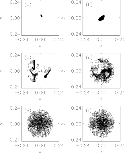
Figure 5: $x-y$ coordinates for a $1600$-orbit ensemble evolved with ${\gamma}=1$ with the lowest energy recorded at six different times. (a) $t=t_{D}$. (b) $t=4t_{D}$. (c) $t=8t_{D}$. (d) $t=16t_{D}$. (e) $t=40t_{D}$. (f) $t=100t_{D}$.

3.4 Chaotic mixing

These results have obvious implications for chaotic mixing. Earlier work (cf. Kandrup & Mahon 1994a, Merritt & Valluri 1998, Kandrup 1998b) would suggest (i) that, as probed by quantities like the phase space dispersions ${\sigma}_{x}$ and ${\sigma}_{px}$, initially localised ensembles of chaotic orbits will diverge exponentially, and (ii) that, as probed by various lower-order moments and/or coarse-grained reduced distribution functions, they will exhibit a roughly exponential evolution towards a near-equilibrium (a near-invariant distribution), both effects proceedings on a mixing time scale $t_{M}$ that correlates with the Lyapunov time scale $t_{L}=1/{\chi}$ associated with the largest Lyapunov exponent. However, to the extent that the typical values of short time Lyapunov exponents can differ substantially for different ensembles, one might anticipate that these ensembles could approach a near-equilibrium at very different rates; and, to the extent that orbits can be ‘stuck’ in a given portion of the chaotic phase space for a very long time, one would not expect that the near-equilibrium should be independent of the choice of chaotic ensemble. Rather, one would anticipate a two- (or more) stage evolution, whereby a rapid approach towards a uniform population of the easily accessible regions is followed by a slower evolution as orbits diffuse along the Arnold web to probe the entire accessible phase space. The approach towards a near-invariant distribution typically proceeds on a comparatively short time scale $t_{M}{\;}{\sim}{\;}1/{\chi}$. The final approach towards a true invariant distribution often proceeds on a time scale $t_{eq}{\;}{\gg}{\;}1/{\chi}$.

These ideas were tested for the triaxial Dehnen potentials by performing simulations which tracked the evolution of ensembles of $1600$ initial conditions localised within phase space cells of typical size $0.01$ or less, and these expectations were all confirmed. Numerical evolution of localised ensembles of initial conditions indicates that quantities like the dispersion ${\sigma}_{x}$ in the coordinate $x$ do indeed diverge exponentially at a rate that correlates with an average short time Lyapunov exponent for the ensemble. Moreover, coarse-grained reduced distribution functions constructed from these orbits appear to converge exponentially towards a nearly constant $f_{\rm inv}$. However, the rate at which the dispersions grow and the rate of convergence towards $f_{\rm inv}$ can both depend on the choice of ensemble as well as the direction(s) in phase space that are probed. For example, for the lowest energy shell with ${\gamma}=1$, there is often a propensity for ensembles starting with small $z$ to diverge comparatively slowly in the $z$-direction, so that ${\sigma}_{z}$ approaches a near-constant value more slowly than ${\sigma}_{x}$ and ${\sigma}_{y}$, and the coarse-grained distribution function converges towards $f_{\rm inv}$ more slowly in the $z$- and $v_{z}$-directions than in any other direction. This is illustrated in FIGURES 5 and 6, which exhibit, respectively, the $x-y$ and $y-z$ coordinates for the same $1600$ orbit ensembles at times $t=t_{D}$, $4t_{D}$, $8t_{D}$, $16t_{D}$, $40t_{D}$, and $100t_{D}$. Alternatively, the spatial dispersions ${\sigma}_{x}$ and ${\sigma}_{z}$ are exhibited in the top two panels of FIGURE 8, which is discussed more carefully in the following Section.

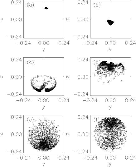
Figure 6: $y-z$ coordinates for the same $1600$-orbit ensemble recorded at six different times. (a) $t=t_{D}$. (b) $t=4t_{D}$. (c) $t=8t_{D}$. (d) $t=16t_{D}$. (e) $t=40t_{D}$. (f) $t=100t_{D}$.

That the near-invariant distributions generated from different chaotic ensembles with essentially the same energy need not be statistically identical is illustrated by the fact that the moments associated with different ensembles need not evolve towards the same near-constant values. An example thereof is exhibited in the top six panels of FIGURE 7, which compares the time-dependent dispersions ${\sigma}_{x}$, ${\sigma}_{y}$, and ${\sigma}_{z}$ for two different ensembles of 6400 orbits, each sampling the lowest energy shell with ${\gamma}=1$. Both ensembles were generated from initial conditions with ${\bf v}=0$, i.e., orbits which, in the absence of a cusp, might be expected to correspond to regular boxes. Each panel is indicative of a moment converging towards a near-constant value, but it is evident that these values are distinctly different for the two different ensembles. One might perhaps worry that these differences could reflect the fact that some of the orbits in these ensembles are actually regular. That this is not the case is clear from the last two panels in FIGURE 7, which exhibit distributions of short time Lyapunov exponents, $N[{\chi}(t)]$, for each of the $6400$-orbit ensembles, computed at $t=200t_{D}$. In each case, a broad range of values are assumed, but the distributions are unimodal and the lowest ${\chi}$ is significantly displaced from ${\chi}=0$.

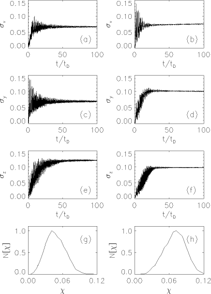
Figure 7: (a) The dispersion ${\sigma}_{x}(t)$ generated for one $6400$ orbit chaotic ensemble sampling the lowest energy shell with ${\gamma}=1$. (b) ${\sigma}_{x}$ for another chaotic ensemble with the same $E$ and ${\gamma}$. (c) and (d) ${\sigma}_{y}$ for the same ensembles. (e) and (f) ${\sigma}_{z}$ for the same ensembles. (e) A distribution of largest short time Lyapunov exponents, $N[{\chi}(t)]$, for $t=200t_{D}$, generated for the first ensemble. (f) The same for the second ensemble.

4 THE EFFECTS OF INTERNAL AND EXTERNAL IRREGULARITIES

The objective here is to determine how the statistical properties of chaotic orbits evolved in these generalised Dehnen potentials change if the evolution equations are modified to allow for low amplitude irregularities which could mimic the effects of internal substructures and/or an external environment. This entailed repeating the simulations of chaotic mixing for unperturbed systems described in the preceding Section but now allowing for low amplitude perturbations. Three specific effects were considered:

${\bullet}$ Periodic driving, intended to mimic the effects of one or two companion objects and/or internal pulsations. This involved allowing for an evolution equation of the form

$${d^{2}x^{a}\over dt^{2}}=-{{\partial}V({\bf r})\over{\partial}x^{a}}+A^{a}\sin({\omega}_{a}t+{\varphi}_{a}),\qquad(a=x,y,z),$$ (3)

incorporating simple pulsations in three orthogonal directions with different amplitudes, frequencies, and phases.

${\bullet}$ Friction and additive white noise, intended to mimic discreteness effects, i.e., gravitational Rutherford scattering. This involved solving a Langevin equation (cf. Chandrasekhar 1943b, van Kampen 1981)

$${d^{2}x^{a}\over dt^{2}}=-{{\partial}V({\bf r})\over{\partial}x^{a}}-{\eta}v^{a}+F^{a},\qquad(a=x,y,z),$$ (4)

with ${\eta}$ a constant coefficient of dynamical friction and ${\bf F}$ a ‘stochastic force.’ Assuming in the usual fashion that ${\bf F}$ corresponds to homogeneous Gaussian noise, its statistical properties are characterised completely by its first two moments, which take the form

$${\langle}F_{a}(t){\rangle}=0\qquad{\rm and}$$

$${\langle}F_{a}(t_{1})F_{b}(t_{2}){\rangle}={\delta}_{ab}\;K(t_{1}-t_{2}),\hskip 14.45377pt(a,b=x,y,z).$$ (5)

The assumption that the noise be white implies that the autocorrelation function $K$ is proportional to a Dirac delta, so that

$$K({\tau})=2{\eta}{\Theta}{\delta}_{D}({\tau}).$$ (6)

The normalisation here ensures that the friction and noise are related by a Fluctuation-Dissipation Theorem at a temperature ${\Theta}$.

${\bullet}$ Coloured noise, intended primarily to mimic the effects of a stochastic external environment. This entailed allowing for forces that are random but, nevertheless, of finite duration, i.e., characterised by a finite autocorrelation time. The specific example considered here corresponds to the so-called Ornstein-Uhlenbeck process (cf. van Kampen 1981), for which $K$ decreases exponentially in time, i.e.,

$$K({\tau})={\alpha}{\eta}{\Theta}\,\exp(-{\alpha}|{\tau}|),$$ (7)

where the autocorrelation time $t_{c}=1/{\alpha}$ sets the time scale on which ${\bf F}$ changes appreciably. The normalisation here ensures that the diffusion constant $D$ that would enter into a Fokker-Planck description,

$$D=\int_{-\infty}^{\infty}\,d{\tau}K({\tau})=2{\Theta}{\eta},$$ (8)

is independent of ${\alpha}$.

White noise was implemented computationally using an algorithm described in Griner, Strittmatter, & Honerkamp (1988). Coloured noise was implemented using an algorithm similar to that described in Pogorelov & Kandrup (1999).

This modeling of perturbations is clearly simplistic but, nevertheless, not completely unreasonable. Earlier work on periodic driving as a source of phase space transport suggests strongly that the exact way in which the system is pulsed matters less than the amplitude and driving frequency. For example, Kandrup, Abernathy, and Bradley (1995) found that, for variants of an anisotropic Plummer potential, similar results obtained when pulsing the core radius and the anisotropy parameter.

Although the detailed forms of the friction and noise can be very important for phenomena like evaporation from a cluster (cf. Chandrasekhar 1943a) or barrier penetration problems (cf. Lindenberg & Seshadri 1981), they appear to be comparatively unimportant in determining the rate of phase space transport. Work on simpler two- and three-dimensional systems (Pogorelov & Kandrup 1999, Kandrup, Pogorelov, & Sideris 1999) shows that making ${\eta}$ a simple but nontrivial function of ${\bf v}$ and/or turning off the friction term altogether has only minimal effects. Moreover, the detailed form of the coloured noise seems largely immaterial. What really matter are the amplitude and the autocorrelation time $t_{c}$, which determines the frequencies at which the perturbation has substantial power. When $t_{c}{\;}{\ll}{\;}t_{D}$, colour matters very little and the effects are similar to white noise. However, when $t_{c}{\;}{\gg}{\;}t_{D}$, so that there is little power at frequencies ${\sim}{\;}1/t_{D}$, the efficacy of the perturbation decreases logarithmically.

4.1 Friction and white noise

Consider first discreteness effects, modeled as friction and white noise. Here the most obvious conclusion is that even weak perturbations can significantly accelerate phase space transport by allowing orbits that are comparatively ‘sticky’ in one or more phase space directions to become ‘unstuck.’ This is illustrated in FIGURE 8, which exhibits the configuration space dispersions ${\sigma}_{x}$ and ${\sigma}_{z}$ for the ensemble of initial conditions used to generate FIGURES 5 and 6, contrasting unperturbed motion with orbits perturbed by friction and additive white noise with constant ${\Theta}=-E$ and three different values of ${\eta}$, namely ${\eta}=0.4\times 10^{-7}$, $0.4\times 10^{-6}$, and $0.4\times 10^{-5}$. Given that, for this choice of ${\gamma}$ and energy, $t_{D}{\;}{\approx}{\;}2.444$, these values correspond respectively to relaxation times $t_{R}=1/{\eta}{\;}{\approx}{\;}10^{7}t_{D}$, $10^{6}t_{D}$ and $10^{5}t_{D}$.

Figure 8: (a) The dispersion ${\sigma}_{x}$ computed for an initially localised ensemble of $1600$ orbits in the lowest energy shell with ${\gamma}=1$ integrated in the absence of any perturbations. (b) The corresponding ${\sigma}_{z}$. (c) ${\sigma}_{x}$ for the same ensemble, now allowing for friction and white noise with temperature ${\Theta}=-E$ and amplitude ${\eta}=10^{-7}$. (d) ${\sigma}_{z}$ for the same friction and noise. (e) ${\sigma}_{x}$ for the same ensemble, with ${\Theta}=-E$ and ${\eta}=10^{-6}$. (f) ${\sigma}_{z}$ for the same friction and noise. (g) ${\sigma}_{x}$ for the same ensemble, with ${\Theta}=-E$ and ${\eta}=10^{-5}$. (h) ${\sigma}_{z}$ for the same friction and noise.

It is apparent that friction and noise with ${\eta}=0.4\times 10^{-7}$ has a relatively small effect, that ${\eta}=0.4\times 10^{-6}$ has a substantially larger effect, and that perturbations with ${\eta}=0.4\times 10^{-5}$ suffice to make ${\sigma}_{z}$ evolve as if the ensemble were hardly sticky at all. This behaviour is also manifested by the visual appearance of the orbit ensemble, as illustrated in FIGURE 9, which, for ${\eta}=10^{-6}$, exhibits the $y$ and $z$ coordinates of the particles at the same times as for FIGURE 6.

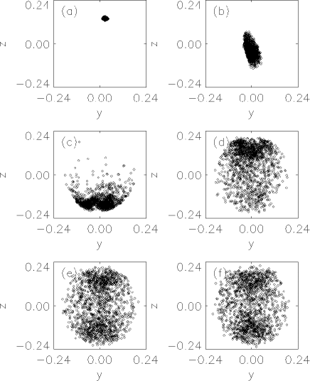
Figure 9: $y-z$ coordinates for the $1600$-orbit ensemble of FIGS. 5 and 6, now evolved with friction and white noise with ${\Theta}=-E$ and ${\eta}=10^{-6}$. (a) $t=t_{D}$. (b) $t=4t_{D}$. (c) $t=8t_{D}$. (d) $t=16t_{D}$. (e) $t=40t_{D}$. (f) $t=100t_{D}$.

Even in the absence of stickiness, discreteness effects can be important by serving to ‘fuzz out’ high frequency structure in quantities like the phase space dispersions and other lower order moments, as well as various reduced distribution functions, thus rendering more efficient the approach towards a near-equilibrium. In particular, such noise can serve to damp the oscillations associated oftentimes with the evolution towards equilibrium, as noted, e.g., by Merritt & Valluri (1996) and Kandrup (1998b). This effect is somewhat apparent in FIGURES 8, which exhibit ${\sigma}_{x}$ and ${\sigma}_{z}$ for a period $t=100t_{D}$, but is even more striking in FIGURES 10, which exhibit ${\sigma}_{y}$ for the shorter interval $0<t<50t_{D}$.

Figure 10: (a) The dispersion ${\sigma}_{y}$ computed for an initially localised ensemble of $1600$ orbits in the lowest energy shell with ${\gamma}=1$ integrated in the absence of any perturbations. (b) ${\sigma}_{y}$ for the same ensemble, now allowing for friction and white noise with temperature ${\Theta}=-E$ and amplitude ${\eta}=10^{-7}$. (c) ${\sigma}_{y}$ for the same ensemble, with ${\Theta}=-E$ and ${\eta}=10^{-6}$. (d) ${\sigma}_{y}$ for the same ensemble, with ${\Theta}=-E$ and ${\eta}=10^{-5}$

.

How large must ${\eta}$ be to have a significant effect? In general, perturbations corresponding to $t_{R}{\;}{\sim}{\;}10^{7}t_{D}$ tend to have (at least) a noticeable effect within ${\sim}{\;}20-30t_{D}$, and perturbations with $t_{R}{\;}{\sim}{\;}10^{6}t_{D}$ can have an appreciable effect on the overall approach towards a near-equilibrium on a comparable time scale. Perturbations with $t_{R}$ as small as $10^{5}t_{D}$ can have drastic effects within $10t_{D}$ or so.

Finally, consistent with Habib, Kandrup, & Mahon (1997), it was found that, for chaotic ensembles, the root mean squared change in energy scales as

$${\delta}E_{rms}{\;}{\approx}{\;}(|E|{\Theta}{\eta}t)^{1/2},$$ (9)

with $E$ the original energy, which implies that noise is important already for ${\delta}E_{rms}{\;}{\sim}{\;}10^{-3}|E|$. This reinforces the interpretation (cf. Pogorelov & Kandrup 1999, Kandrup, Pogorelov, and Sideris 1999) that this phase space transport is not driven by changes in energy, which only become large on a relaxation time $t_{R}$, but instead reflects diffusion along Arnold webs on (nearly) constant energy hypersurfaces.

The basic conclusion derived from these investigations is that discreteness effects can be important within a period as short as $50-100t_{D}$ provided only that the relaxation time is no larger than $10^{6}-10^{7}t_{D}$ or so. This suggests strongly that, especially near the centers of cuspy galaxies, discreteness effects should be important on time scales considerably shorter than $t_{H}$, the age of the Universe.

4.2 Periodic driving

Overall, periodic driving has the same qualitative effects on orbit ensembles as does white noise. Periodic driving can enable “sticky” orbits to become unstuck, thus facilitating phase space transport; and, even in the absence of topological obstructions, driving can help fuzz out high frequency, short wavelength structures. Not surprisingly, for fixed amplitude $A$ periodic driving has the largest effect for driving frequencies ${\omega}_{i}$ with $1/{\omega}_{i}{\;}{\sim}{\;}t_{D}$, so that there is a substantial resonant coupling between the driving frequencies and the natural frequencies of the unperturbed orbits.

One important difference between noise and periodic driving is that, whereas noise represents an incoherent process, involving a random superposition of frequencies, periodic driving with fixed frequencies is a coherent process. That periodic driving is coherent would suggest that its coupling to orbits should scale linearly in amplitude, i.e., ${\propto}{\;}A$, a fact that has been confirmed numerically (cf. Kandrup, Abernathy, & Bradley 1995). Because noise is incoherent, its coupling scales instead as ${\eta}^{1/2}$ (cf. Habib, Kandrup, & Mahon 1997). For $1/{\omega}_{i}{\;}{\sim}{\;}t_{D}$ it is thus natural to expect that, if noise requires an amplitude ${\eta}{\;}{\sim}{\;}10^{-p}$ to induce a substantial effect within a given time interval, periodic driving will require an amplitude $A{\;}{\sim}{\;}10^{-p/2}$ to have a comparable effect.

Overall, this scaling tends to hold at least roughly true. However, one discovers (i) that the minimum amplitude required to achieve a given effect can exhibit a comparatively sensitive dependence on the choice of frequencies, and (ii) that the “typical” effect of periodic driving is slightly weaker than is predicted by this scaling. These facts are both easily understood. The fact that noise involves a superposition of many different frequencies implies that the details tend to “wash out,” and that one is more likely to have power at one of the “more effective” frequencies.

4.3 Friction and coloured noise

As for other two- and three-dimensional potentials, coloured noise sampling the Ornstein-Uhlenbeck process has virtually the same effect as does white noise with the same amplitude, provided only that the autocorrelation time $t_{c}$ is short compared with the dynamical time $t_{D}$. However, when $t_{c}$ becomes comparable to $t_{D}$ the effects of the noise begin to decrease significantly; and, for $t_{c}{\;}{\gg}{\;}t_{D}$ the effects of the noise are substantially reduced.

Examples of this behaviour, which corroborate the interpretation of noise-induced phase space transport as a resonance phenomenon, are presented in FIGURE 11, which exhibits ${\sigma}_{z}$ generated from the same ensemble of initial conditions used to generate FIGURE 8, now evolved with coloured noise. The first three panels represent friction and noise with ${\Theta}=E$ and ${\eta}=0.4\times 10^{-5}$ for three choices of autocorrelation time, namely $t_{c}{\;}{\approx}{\;}0.4t_{D}$, $1.2t_{D}$, and $4.0t_{D}$. The fourth and fifth panels were generated for ${\Theta}=-E$ and $t_{c}{\;}{\approx}{\;}4.0t_{D}$ but larger values of ${\eta}=0.4\times 10^{-4}$ and $0.4\times 10^{-3}$. The final panel is generated for ${\Theta}=-E$, ${\eta}=1.2\times 10^{-3}$, and $t_{c}{\;}{\approx}{\;}12t_{D}$. It is clear that for these values, which are not inappropriate for modeling the effects of an external environment on a galaxy embedded in a rich cluster, perturbations can have a dramatic effect.

Figure 11: (a) The dispersion ${\sigma}_{z}$ computed for the same initial conditions as FIG. 8, now allowing for coloured noise with ${\Theta}=-E$, ${\eta}=0.4\times 10^{-5}$, and $t_{c}=1/{\alpha}=1.0{\;}{\approx}{\;}0.4t_{D}$. (b) The same for ${\eta}=0.4\times 10^{-5}$, and $t_{c}=3.0{\;}{\approx}{\;}1.2t_{D}.$ (c) The same for ${\eta}=0.4\times 10^{-5}$, and $t_{c}=10.0{\;}{\approx}{\;}4t_{D}.$ (d) The same for ${\eta}=0.4\times 10^{-4}$, and $t_{c}=10.0{\;}{\approx}{\;}4t_{D}.$ (e) The same for ${\eta}=0.4\times 10^{-3}$, and $t_{c}=10.0{\;}{\approx}{\;}4t_{D}.$ (f) The same for ${\eta}=1.2\times 10^{-3}$, and $t_{c}=30.0{\;}{\approx}{\;}12t_{D}.$

4.4 The approach towards an invariant distribution

Even though low amplitude perturbations can accelerate the approach towards a near-invariant distribution, they need not suffice to make different ensembles evolve towards the same distribution within a time $t{\;}{\sim}{\;}100t_{D}$ or so. For example, even though friction and noise corresponding to a relaxation time as long as $t_{R}{\;}{\sim}{\;}10^{6}t_{D}$ or more can have an appreciable effect on the efficacy with which the ensemble approaches a near-invariant distribution, perturbations corresponding to a $t_{R}$ as short as $10^{4}t_{D}$ may not suffice to yield a convergence of moments for two different chaotic ensembles with the same ${\gamma}$ and $E$. This is, e.g., illustrated in FIGURE 12, which exhibits ${\sigma}_{z}$ for the same two sets of initial conditions used to generate FIGURE 7, but now allowing for friction and white noise with $t_{R}=10^{6}t_{D}$, $10^{5}t_{D}$, and $10^{4}t_{D}$. The $t=200t_{D}$ dispersions for the two ensembles are appreciably different even for $t_{R}=10^{4}t_{D}$, where the friction and noise have caused the energy of a typical orbit to change by more than 4%. Both ensembles began with energies $E{\;}{\approx}{\;}-0.996$. When evolved allowing for perturbations corresponding to $t_{R}=10^{4}t_{D}$, the two final energy dispersions were ${\sigma}_{E}=0.045$ and ${\sigma}_{E}=0.046$.

Figure 12: (a) The dispersion ${\sigma}_{z}$ computed for one initially localised ensemble of chaotic orbits in the lowest energy shell with ${\gamma}=1$, allowing for friction and white noise corresponding to $t_{R}=10^{6}t_{D}$ (b) ${\sigma}_{z}$ for another chaotic ensemble with the same ${\gamma}$, $E$ and $t_{R}$. (c) and (d) ${\sigma}_{z}$ for the same two ensembles of initial conditions, now integrated with $t_{R}=10^{5}t_{D}$.(e) and (f) ${\sigma}_{z}$ for the same two ensembles of initial conditions, integrated with $t_{R}=10^{4}t_{D}$.

5 THE EFFECTS OF A SUPERMASSIVE BLACK HOLE

The objective here is to determine how the basic picture described in the preceding Sections is altered if one allows for a modified potential of the form

$$V({\bf r})=V_{\gamma}({\bf r})-{M_{BH}\over(x^{2}+y^{2}+z^{2}+{\epsilon}^{2})^{1/2}},$$ (10)

where $V_{\gamma}$ denotes the unperturbed potential associated with the density distribution (1). $M_{BH}$ is the black hole mass, expressed in units of the total galactic mass (since eq. (1) implies that $\int\,d^{3}r\,{\rho}({\bf r})=1$) and ${\epsilon}=10^{-3}$ is a softening parameter. The choice of a relatively large value for ${\epsilon}$ was motivated by computational considerations. Noisy simulations are effected with a fixed time step integrator (cf. Honerkamp 1994), but integrations with a force which becomes very large for $r\to 0$ require very small time steps to maintain reasonable accuracy. Indeed, even for this comparatively large value of ${\epsilon}$, the black hole simulations with $M_{BH}=10^{-3}$ and ${\gamma}=1$ required a time step an order of magnitude smaller than for comparable simulations with $M_{BH}=0$. An investigation of the effects of varying ${\epsilon}$ in the simpler potential (11), which exhibits qualitatively similar behaviour, indicates that the precise value of ${\epsilon}$ is comparatively unimportant, provided only that $r_{min}$, the closest approach of an orbit to the black hole, is large compared with ${\epsilon}$. This condition suggests that it suffices to consider ${\epsilon}{\;}{\ll}{\;}10^{-2}$.

Four sorts of experiments were performed, namely: (1) computations of “libraries” of $1000$ representative orbits of length $t=200t_{D}$, to determine the relative numbers of regular and chaotic orbits; (2) long time integrations for $t=102400t_{D}$ to obtain estimates of the true ${\chi}$ for chaotic orbits, as well as to extract distributions of short time Lyapunov exponents; (3) $1600$-orbit simulations of chaotic mixing, allowing for a black hole but no additional perturbations; and (4) $1600$-orbit simulations of chaotic mixing that included both a black hole and low amplitude time-dependent irregularities. Attention focused primarily on two choices of black hole mass, namely $M_{BH}=10^{-3}$ and $M_{BH}=10^{-2}$.

5.1 How chaotic are the orbits?

Consistent with Merritt (1998), it was found that allowing for a nonzero $M_{BH}$ makes the flow ‘more chaotic’ in the sense that, for chaotic orbits, the typical values of the Lyapunov exponents ${\chi}$ increase. Not surprisingly, this effect is most pronounced in the lower energy shells where the orbits tend to pass the closest to the hole. For all four values of ${\gamma}$, introducing a black hole with a mass as large as $M_{BH}=10^{-2}$ only increases the typical values of ${\chi}$ in the ninth shell by less than a factor of two. However, especially for smaller values of ${\gamma}$, the black hole can have much larger effects on the lowest two energy shells. For ${\gamma}=0$, a black hole with $M_{BH}=10^{-2}$ increases the values of ${\chi}$ in the lowest energy shell by an order of magnitude. For ${\gamma}=1$, the increase is by a factor of three. For ${\gamma}=2$, a black hole with mass $M_{BH}=10^{-2}$ increases the typical ${\chi}$ by less than a factor of two, and $M_{BH}=10^{-3}$ has a comparatively minimal effect.

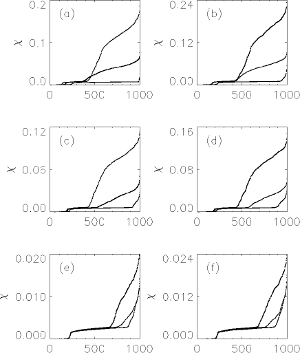
Figure 13: (a) Short time ${\chi}(t=200t_{D})$ for $1000$ orbits in the lowest energy shell with ${\gamma}=0$, arranged by increasing values of ${\chi}$. From bottom to top, the three curves represent $M_{BH}=0$, $M_{BH}=10^{-3}$, and $M_{BH}=10^{-2}$. (b) The same for the lowest energy shell with ${\gamma}=0.3$. (c) The second lowest energy shell with ${\gamma}=0$. (d) The second lowest energy shell with ${\gamma}=0.3$. (e) The ninth lowest energy shell with ${\gamma}=0$. (f) The ninth lowest energy shell with ${\gamma}=0.3$.

The presence of a supermassive black hole can also impact significantly the relative abundance of “strongly chaotic” orbit segments with ${\chi}$ significantly larger than zero. For the two less cuspy models, ${\gamma}=0$ and ${\gamma}=0.3$, even a black hole mass as small as $M_{BH}=10^{-3}$ suffices to trigger a significant increase in the relative number of strongly chaotic segments, particularly for the lower energy shells. For ${\gamma}=1$ and ${\Delta}t=200t_{D}$, such a black hole increases significantly the number of chaotic orbits in the two lowest energy shells, but its effect on the ninth energy shell is much less pronounced. For ${\gamma}=2$, even a black hole as large as $M_{BH}=10^{-2}$ seems to have no appreciable effect on the relative number of strongly chaotic orbits in any of the three energy shells.

The net conclusion, in agreement with Merritt (1998, 1999), is that, under appropriate circumstances, supermassive black holes with $M_{BH}{\;}{\sim}{\;}10^{-3}-10^{-2}$ can significantly impact both the relative number of chaotic orbits that exist and the typical values of their largest short time Lyapunov exponent. Merritt’s argument that the principal effect of the supermassive black hole is to enhance the strength of the central cusp would seem to explain why, for ${\gamma}=2$, a black hole of fixed mass has a much smaller effect than for smaller values of ${\gamma}$: In this case, a very pronounced density cusp is already there!

But what about the question of ‘stickiness’? Does the presence of a supermassive black hole tend to make distinctions between regular and chaotic orbits more evident, or is it still possible for a chaotic orbit to ‘look regular’ for very long times? Here the first obvious point is that, viewed over times ${\sim}{\;}100t_{D}-200t_{D}$, the computed values of ${\chi}$ for an ensemble containing both regular and chaotic orbits do not divide neatly into two disjoint classes with small and large values of ${\chi}$ and nothing in between.

This is, e.g., manifest from FIGURES 13 and 14, which summarise information about the numbers of orbit segments with different values of ${\chi}$ for integrations of duration $t=200t_{D}$. These FIGURES encapsulate information about the short time Lyapunov exponents computed for $36$ different ensembles of $1000$ initial conditions – one each for the first, second, and ninth energy shells for the four different values of ${\gamma}$ with $M_{BH}=0$, $M_{BH}=10^{-3}$, and $M_{BH}=10^{-2}$. For each ensemble, the orbits were ordered by the size of the computed value of ${\chi}$ and the resulting ${\chi}$’s were then plotted as a function of particle number from $1$ to $1000$. Inspection of these FIGURES thus allows one to infer the overall range of ${\chi}$’s that was observed, the relative number of orbits in any given interval ${\Delta}{\chi}$, and how this number varies with changes in $E$, $M_{BH}$, and/or ${\gamma}$. In interpreting these FIGURES, it should be noted that they were generated as collections of tiny diamonds, not solid lines. The near-complete absence of any gaps thus manifests the fact that the orbits seemingly sample a near-continuous range of ${\chi}$’s, and that there is no pronounced break between regular and chaotic orbits. The presumption is that all points not lying along a nearly horizontal line with very small ${\chi}$ correspond to chaotic orbits, some relatively sticky and some otherwise.

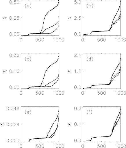
Figure 14: (a) Short time ${\chi}(t=200t_{D})$ for $1000$ orbits in the lowest energy shell with ${\gamma}=1$. From bottom to top, the three curves represent $M_{BH}=0$, $M_{BH}=10^{-3}$, and $M_{BH}=10^{-2}$. (b) The same for the lowest energy shell with ${\gamma}=2$. (c) The second lowest energy shell with ${\gamma}=1$. (d) The second lowest energy shell with ${\gamma}=2$. (e) The ninth lowest energy shell with ${\gamma}=1$. (f) The ninth lowest energy shell with ${\gamma}=2$.

The absence of a pronounced gap in ${\chi}$ between the regular and chaotic orbits indicates that, as for the case with $M_{BH}=0$, the distribution of short time ${\chi}$’s must extend down to zero and, as such, one might perhaps suppose that $N[{\chi}]$, the distribution of short time Lyapunov exponents for chaotic orbit segments, is again at least bimodal. That this is often so is illustrated in FIGURES 15 and 16, which exhibit the analogues of several panels from FIGURES 1 and 2 for long time integrations with $M_{BH}=10^{-3}$ and $M_{BH}=10^{-2}$.

Figure 15: (a) $N[{\chi}({\Delta}t)]$, the distribution of short time Lyapunov exponents, for chaotic orbits in the lowest energy shell with ${\gamma}=0$ and $M_{BH}=10^{-3}$ for sampling time ${\Delta}t=100t_{D}$. (b) $N[{\chi}({\Delta})]$ for chaotic orbits in the lowest energy shell with ${\gamma}=0$, $M_{BH}=10^{-2}$, and ${\Delta}t=100t_{D}$. (c) The same for chaotic orbits in the ninth energy shell with ${\gamma}=0$ and $M_{BH}=10^{-3}$ (d) The same for chaotic orbits in the ninth energy shell with ${\gamma}=0$ and $M_{BH}=10^{-2}$ (e) - (h) The same as (a) - (d) for ${\gamma}=0.3$.

Figure 16: (a) $N[{\chi}({\Delta}t)]$, the distribution of short time Lyapunov exponents, for chaotic orbits in the lowest energy shell with ${\gamma}=1$ and $M_{BH}=10^{-3}$ for sampling time ${\Delta}t=100t_{D}$. (b) $N[{\chi}({\Delta})]$ for chaotic orbits in the lowest energy shell with ${\gamma}=1$, $M_{BH}=10^{-2}$, and ${\Delta}t=100t_{D}$. (c) The same for chaotic orbits in the ninth energy shell with ${\gamma}=1$ and $M_{BH}=10^{-3}$ (d) The same for chaotic orbits in the ninth energy shell with ${\gamma}=1$ and $M_{BH}=10^{-2}$ (e) - (h) The same as (a) - (d) for ${\gamma}=2$.

But how do things vary with the sampling time ${\Delta}t$? Does the presence of a supermassive black hole serve to accelerate phase space transport significantly, thus making the time scale to diffuse from one portion of phase space to another much shorter? The answer here seems to be: no! One again discovers that, over very long time scales, $t{\;}{\sim}{\;}20000t_{D}$ or longer, different segments of the same chaotic orbit can look extremely different, varying in appearance from wildly chaotic to nearly regular. This is manifested by the time-dependence of the dispersions ${\sigma}_{\chi}({\Delta}t)$ which, as for the case when $M_{BH}=0$, typically decay much more slowly than as ${\Delta}t^{-1/2}$. Examples of the observed behaviour, generated as for FIGURES 3 and 4, are exhibited in FIGURE 17, which show ${\sigma}_{\chi}$ for several different choices of ${\gamma}$, $E$, and $M_{BH}$.

Figure 17: (a) The dispersion ${\sigma}_{\chi}$ for chaotic orbits in the lowest energy shell with ${\gamma}=1$ and $M_{BH}=10^{-3}$, computed as a function of sampling time ${\Delta}t$. (b) ${\sigma}_{\chi}$ for chaotic orbits in the lowest energy shell with ${\gamma}=1$ and $M_{BH}=10^{-2}$. (c) The same for the ninth energy shell and $M_{BH}=10^{-3}$. (d) The same for the ninth energy shell and $M_{BH}=10^{-2}$. (e) - (h) The same as (a) - (d) for ${\gamma}=2$.

Figure 18: (a) The dispersion ${\sigma}_{x}$ computed for an unperturbed ensemble of $1600$ orbits in the second lowest energy shell for ${\gamma}=2$, evolved in the absence of a supermassive black hole. (b) The same for an ensemble in the ninth energy shell. (c) The same as (a), but now allowing for a black hole with mass $M_{BH}=10^{-3}$. (d) The same as (b), but with $M_{BH}=10^{-3}$. (e) The same as (c), but with $M_{BH}=10^{-2}$. (f) The same as (d), but with $M_{BH}=10^{-2}$.

5.2 Chaotic mixing

The effects of a supermassive black hole on chaotic mixing are completely predictable. The presence of such a black hole fails to facilitate significantly the evolution of initially localised ensembles towards a true equilibrium in the sense that the phase space is still very sticky, so that chaotic orbits can remain confined in restricted phase space regions for very long times. However, a supermassive black hole does tend to accelerate the approach towards a near-equilibrium. The correlation between the Lyapunov time $t_{L}=1/{\chi}$ and the time scale $t_{M}$ on which a chaotic ensemble evolves persists for $M_{BH}{\;}{\neq}{\;}0$, but this means that larger ${\chi}$’s correspond to a more rapid evolution. One example of this behaviour is shown in FIGURE 18, which exhibits ${\sigma}_{x}$ for the same initial ensembles evolved with ${\gamma}=2$ and variable $M_{BH}=0$, $M_{BH}=10^{-3}$, and $M_{BH}=10^{-2}$.

The effects of weak perturbations on chaotic mixing with a supermassive black hole are also predictable. As is the case for $M_{BH}=0$, such perturbations can facilitate phase space transport, thus accelerating the approach towards equilibrium; and, even in the absence of any obvious ‘stickiness,’ they can play an important role in ‘fuzzing out’ high frequency structures. Moreover, the minimum amplitudes required to have an appreciable effect are comparable to what is required when $M_{BH}=0$. In particular, discreteness effects, modeled as friction and white noise, should be important on a time scale $<100t_{D}$ provided only that $t_{R}<10^{6}-10^{7}t_{D}$.

6 DISCUSSION

The ‘stickiness’ observed in these triaxial Dehnen potentials is so striking that one may wonder how generic it is. It is thus reassuring that the same qualitative behaviour can arise for the simple model comprised of an anisotropic oscillator and a spherical Plummer potential. For example, the qualitative form of $N[{\chi}({\Delta}t)]$, the distribution of short time Lyapunov exponents for the triaxial Dehnen potentials, can be reproduced by orbits evolved in a potential of the form

$$V({\bf r})={1\over 2}{\Bigl{(}}{\omega}_{x}^{2}x^{2}+{\omega}_{y}^{2}y^{2}+{\omega}_{z}^{2}z^{2}{\Bigr{)}}-{M_{BH}\over\sqrt{r^{2}+{\epsilon}^{2}}},$$ (11)

with ${\omega}_{x}^{2}=1.0$, ${\omega}_{y}^{2}=1.25$, ${\omega}_{z}^{2}=0.75$, and ${\epsilon}=10^{-3}$, for appropriate choices of energy $E$ and black hole mass $M_{BH}$.

For $M_{BH}=0$ and $M_{BH}\to\infty$, motion in this potential is completely integrable. However, $V({\bf r})$ is nonintegrable for intermediate values and, for a reasonable range of black hole masses, admits a coexistence of large numbers of both regular and chaotic orbits. In this range, one finds typically that increasing $M_{BH}$ makes the system more chaotic in the sense that the values of ${\chi}$ tend to increase, but that, when expressed in units of $1/t_{D}$, the changes in ${\chi}$ are not all that large. One discovers further that, generically, the chaotic orbits tend to be very sticky, so that an integration for a time $t=10000t_{D}$ or longer does not suffice to yield convergence towards the asymptotic ${\chi}$, defined in a $t\to\infty$ limit. In both these ways, this potential is very Dehnenesque.

As an indication of the degree to which this potential yields similar distributions of short time Lyapunov exponents $N[{\chi}({\Delta}t)]$, consider FIGURE 19, which exhibits $N[{\chi}({\Delta}t)]$ for ensembles of chaotic orbits. These ensembles were generated from initial conditions that uniformly sampled the $y-z$ plane, setting $x=v_{y}=v_{z}=0$ and, for given energy $E$, solving for $v_{x}(y,z,E)>0$. Each orbit was integrated for a time $t=4096$ and the computed values of ${\chi}$ at that time were used to identify which initial conditions appeared chaotic. The orbits identified as chaotic were then divided into $16$ segments of length ${\Delta}t=256$ which, for the range of energies and black hole masses exhibited in these FIGURES, corresponded to a period of order $100t_{D}$, and short time Lyapunov exponents were identified for each segment. The resulting collection of ${\chi}$’s was then binned to generate $N[{\chi}]$ for ${\Delta}t=256$. The first panel, for $M_{BH}=10^{-1.5}$ and $E=0.0044$, closely resembles the bimodal distributions $N[{\chi}({\Delta}t)]$ observed for the lower energy shells in the Dehnen potentials. The second panel, generated for $M_{BH}=10^{-2}$ and $E=0.65$, resembles more closely the distributions for the higher energy shells, especially in the presence of a black hole.

The results described in this paper have potentially significant implications for modeling galaxies using Schwarzschild’s (1979) method or any comparable technique. One obvious point is that, in the absence of any time-dependent perturbations, phase space transport can be extremely inefficient, so that computing an ensemble of orbits even for $1000t_{D}$ or longer may not suffice to obtain a reasonable approximation to an invariant distribution. Great care needs to be taken in endeavoring to create truly time-independent building blocks. At least for cusps that are not too steep, inserting a supermassive black hole typically makes orbits more chaotic in the sense that the Lyapunov exponents become larger and, in addition, tends to increase the relative abundance of chaotic orbits. However, the presence of the black hole does not seem to significantly accelerate the rate of phase space transport.

Figure 19: (a) Short time $N[{\chi}(t=256)]$ for a collection of chaotic orbits evolved in the toy potential (11) with $M_{BH}=10^{-1.5}$ and $E=0.044$. (b) The same for $M_{BH}=10^{-2}$ and $E=0.065$.

The other obvious point is that even comparatively weak time-dependent perturbations tend to significantly accelerate phase space diffusion, allowing orbits to probe different phase space regions on times short compared with the time scale for phase space transport in the absence of any perturbations. This basic fact, first recognised in the context of simple maps (cf. Lieberman & Lichtenberg 1972) and subsequently explored for simple two- and three-degree-of-freedom systems (cf. Habib, Kandrup, & Mahon 1997), persists for seemingly realistic cuspy, triaxial potentials. This suggests immediately that irregularities associated with the real world could serve to destabilise pseudo-equilibria constructed using near-invariant, rather than truly invariant, building blocks, even if, in the absence of perturbations, such equilibria could persist for times ${\gg}{\;}t_{H}$.

But what are the effects of perturbations like friction and noise? Do they simply accelerate the evolution of an unperturbed system or do they alter the final state? Noise induces significant changes in the energy and any other global isolating integrals on a relaxation time $t_{R}=1/{\eta}$ and, as such, it is clear that noise must change the form of the final state for later times. However, there is good reason to anticipate that, for times $t{\;}{\ll}{\;}t_{R}$, noise simply speeds things up without significantly altering the ultimate outcome. In other words, an ensemble evolved for a time $t_{H}$ in the presence of weak noise with $t_{R}{\;}{\gg}{\;}t_{H}$ might be expected to achieve a final state closely resembling the state which an unperturbed ensemble would have achieved only after a time $100t_{H}$, or even longer. The basic idea is that the perturbations drive phase space transport by helping stars to find phase space holes, thus accelerating the approach towards an equilibrium, but that, at least to the extent that the perturbations do not significantly alter the values of the energy and other isolating integrals, they will not impact the form of the final equilibrium.

An analogy with kinetic theory were perhaps appropriate. When analysing interactions of particles in a dilute gas, one speaks of microreversibility, which implies that the transition rates $W({\bf v}_{1},{\bf v}_{2}\to{\bf v}_{3},{\bf v}_{4})$ and $W({\bf v}_{3},{\bf v}_{4}\to{\bf v}_{1},{\bf v}_{2})$ must be equal. This is a statement about the phase space kinematics, and is without reference to the dynamics. Statistical equilibrium requires detailed balance, characterised by populations $f({\bf v}_{i})$ satisfying $f({\bf v}_{1})f({\bf v}_{2})W({\bf v}_{1},{\bf v}_{2}\to{\bf v}_{3},{\bf v}_{4})=f({\bf v}_{3})f({\bf v}_{4})W({\bf v}_{3},{\bf v}_{4}\to{\bf v}_{1},{\bf v}_{2}).$

In the context of phase space diffusion, the analogue of microreversibility is the notion that the transition rates $W(A\to B)$ and $W(B\to A)$ across a leaky barrier separating regions $A$ and $B$ must be equal. Equilibrium involves a detailed balance with equal (and constant) number densities on both sides of the boundary, so that the product of number density and transition rate is the same. That $W(A\to B)=W(B\to A)$ is incorporated explicitly in every theory of phase space transport, including, e.g., the “turnstile model” for diffusion through cantori, which is the most successful to date (MacKay, Meiss, & Percival 1984). The expectation, then, is that low amplitude perturbations will help stars breach these leaky barriers, but that they will not alter the balance associated with an equilibrium. One could, perhaps, envision carefully tailored “designer noise” so constructed as to favour motion in one direction over the other, but this would seem contrived. The noise used in this paper, and most other investigations of accelerated phase space transport, was chosen to act equally on stars on both sides of the boundary; and, as such, should not serve to alter the final balance.

There is also concrete numerical evidence (cf. Habib, Kandrup, & Mahon 1996, 1997) suggesting that weak noise simply accelerates phase space transport rather than leading to a new equilibrium. This derives from comparing the same ensemble of initial conditions evolved in three different ways, viz: (i) for comparatively short times, $t{\;}{\leq}{\;}100t_{D}$, in the absence of any perturbations, (ii) for longer times, $t>1000t_{D}$, in the absence of perturbations, and (iii) for short times, again $t{\;}{\leq}{\;}100t_{D}$, in the presence of weak noise for which $t_{R}{\;}{\gg}{\;}100t_{D}$. For some choices of potential and/or ensemble, one finds that the short and long time unperturbed simulations result in very similar end states, as probed, e.g., by lower order moments and coarse-grained distribution functions. In this case, weak noise has only a minimal effect. In other cases, however, the short and long times unperturbed simulations yield substantially different end states. In these cases, one finds invariably that the noisy simulations yield a final state that more closely resembles the late time unperturbed state than did the shorter time unperturbed evolution. Moreover, for noise of sufficient strength, one discovers oftentimes that the noisy end state and the long time unperturbed endstate are almost identical.

This motivates a specific proposal, namely that, when using Schwarzschild’s method to construct models that contain significant numbers of chaotic orbits, one should generate “noisy libraries,” which are more likely to constitute reasonable approximations to invariant distributions than are libraries generated without any perturbations. There is no guarantee that the noise will yield truly time-independent building blocks. However, it seems reasonable to anticipate that allowing for weak noise will yield libraries that are, at least, better approximations to invariant distributions.

In contemplating the implications of the computations described in this paper for real galaxies, it is important to recall that the notion of an equilibrium is an idealisation which is never achieved in the real world. Assuming that the evolution is not strongly dissipative, so that Liouville’s Theorem holds at least approximately, there can at best be a coarse-grained approach towards an equilibrium (cf. Lynden-Bell 1967). One might anticipate an approach towards equilibrium in the sense that various moments and/or coarse-grained distributions become systematically more nearly time-independent, but there can be no true pointwise approach towards equilibrium. Moreover, realistic systems are continually subjected to various time-dependent perturbations reflecting both internal and external irregularities, so that, even allowing for dissipation, one could at best view a galaxy as being “near” equilibrium. The basic question is whether it be reasonable to assume that a real galaxy evolves towards a complex time-dependent state which can be approximated realistically as an equilibrium.

Evolving towards a true triaxial equilibrium might seem relatively difficult! It would seem unreasonable to model realistic triaxial systems as equilibria that depend only on one global integral and nothing else. A one-integral $f(E)$ depending only on energy $E$ must be spherical (cf. Perez & Aly 1996). It is possible to construct rotating triaxial equilibria $f(E_{J})$ which involve only the Jacobi integral $E_{J}$, but such equilibria apparently cannot be sufficiently centrally condensed to mimic real physical systems (cf. Vandervoort 1980, Ipser & Managan 1981). Potentials that admit two or three global integrals are a set of measure zero in the set of three-dimensional potentials, and there is a precise sense in which near-integrable systems are substantially rarer for three- and higher-degree-of-freedom systems than for systems with two degrees of freedom (Poincaré 1892).

There remains the possibility of trying to construct equilibria involving non-standard local integrals in addition to the conventional global isolating integrals, perhaps excluding the chaotic orbits altogether. This possibility seems implicit in virtually all work on cuspy triaxial systems hitherto (cf. Zhao 1996, Siopis 1998) and an attempt has been made recently to do this in a more systematic fashion (Häfner et al 1999). Most, if not all, of the potentials that have been considered, including the triaxial Dehnen potentials, have chaotic orbits with two positive Lyapunov exponents and, consequently, can admit only one global isolating integral. However, many dynamicists seem to have the intuitive expectation that such equilibria would be hard to realise, since they entail a “fine-tuning” on a comparatively microscopic level. As such, one might therefore ask: is it reasonable to expect that the true time-dependent distribution function associated with a real galaxy actually manages to approach one of these finely tuned distributions involving local integrals?

Irrespective of the answer to this question, it would seem substantially easier to approach a near-equilibrium than a true equilibrium. One would anticipate intuitively that there are many more near-equilibria than true equilibria, and these could be supported approximately with two types of building blocks, namely (i) building blocks that are only approximately time-independent and/or (ii) building blocks which, albeit exactly time-independent, only reproduce the potential approximately. In this regard, it should perhaps be stressed that there is no guarantee that, in the absence of dissipation, a real galaxy will evolve towards a time-independent equilibrium. One could, at least in principle, envision an evolution towards a final state that entails undamped, finite amplitude oscillations about some time-independent equilibrium (cf. Louis & Gerhart 1988, Sridhar 1989).

These observations are related to two significant limitations implicit in Schwarzschild’s method or any obvious variant thereof: (1) There is no guarantee that any solution constructed using Schwarzschild’s method corresponds to a true equilibrium. It is possible that, strictly speaking, the assumed potential admits no true equilibria, and that the numerical algorithm has only constructed an approximate equilibrium (or worse). (2) The fact that, for some assumed potential, one’s orbit library could not be used to generate a Schwarzschild equilibrium does not imply that an equilibrium does not exist; and even if there is no equilibrium this does not preclude the possibility that there exist “nearby” potentials that correspond to a system which (at least on the average) only evolves comparatively slowly.

The enormous stickiness manifested by chaotic orbits in (at least some) cuspy triaxial potentials can facilitate the construction of approximate equilibria. However, there is every reason to think that low amplitude perturbations associated with both internal and external irregularities could trigger nontrivial evolutionary effects on a time scale ${\ll}{\;}t_{H}$.

From this slightly different chain of reasoning, one is led to a conclusion similar to that of Merritt (1996), namely that galaxies could exhibit a two-stage evolution, a rapid approach towards a roughly, but not truly, time-independent equilibrium on a time scale ${\sim}{\;}t_{D}$ which is succeeded by a substantially slower evolution as the system “searches” for a true equilibrium. Using this line of reasoning exclusively, there is no obvious guarantee that this slower evolution will lead to configurations more nearly axisymmetric – one might instead see an evolution through a sequence of comparably triaxial equilibria. However, the apparent fact that very cuspy galaxies tend to be more nearly axisymmetric, at least in the center, could reflect in part the fact that, in these high density central regions, dissipation was sufficiently strong to allow the system to “develop a global conserved quantity.”

References

- [1] Arnold, V. I., 1964, Russ. Math. Surveys 18, 85.
- [2] Athanassoula, E., Bienyamé, O., Martinet, L., Pfenniger, D. 1983, A&A 127, 349
- [3] Bender, R. et al. 1989, A&A 217, 35
- [4] Binney, J., 1978, Comments Astrophys. 8, 27.
- [5] Binney, J., Tremaine, S., 1987, Galactic Dynamics. Princeton University Press, Princeton.
- [6] Byun, Y.-I. et al. 1996, AJ 111, 1889
- [7] Chandrasekhar, S. 1943a, Principles of Stellar Dynamics. University of Chicago, Chicago
- [8] Chandrasekhar, S. 1943b, Rev. Mod. Phys. 15, 1
- [9] Contopoulos, G., 1971, AJ 76, 147.
- [10] Dehnen, W. 1993, MNRAS 265, 250
- [11] de Zeeuw, T., 1985, MNRAS 216, 273
- [12] Gebhardt, K. et al. AJ 112, 105
- [13] Grassberger, P., Badii, R., Politi, A., 1988, J. Stat. Phys. 51, 135
- [14] Griner, A., Strittmatter, W., Honerkamp, J. 1988, J. Stat. Phys. 51, 95
- [15] Habib, S., Kandrup, H. E., Mahon, M. E. 1996, Phys. Rev. E 53, 5473
- [16] Habib, S., Kandrup, H. E., Mahon, M. E. 1997, ApJ 480, 155.
- [17] Habib, S., Ryne, R. 1995, Phys. Rev. Lett 74, 70
- [18] Häfner, R., Evans, N. W., Dehnen, W., Binney, J. 1999, MNRAS, submited (astro-ph/9905086)
- [19] Hasan, H., Norman, C., 1990, ApJ 361, 69.
- [20] Hénon, M., Heiles, C., 1964, AJ 69, 73.
- [21] Honerkamp, J. 1994, Stochastic Dynamical Systems. VCH Publishers, New York.
- [22] Ipser, J. R., Managan, R. A. 1981, ApJ 250, 362.
- [23] Kandrup, H. E. 1998a, MNRAS 299, 1139
- [24] Kandrup, H. E. 1998b, MNRAS 301, 960
- [25] Kandrup, H. E., Abernathy, R. A., Bradley, B. O. 1995, Phys. Rev. E 51, 5287
- [26] Kandrup, H. E., Eckstein, B. L., Bradley, B. O., 1997, A&A, 320, 65.
- [27] Kandrup, H. E., Mahon, M. E. 1994a, Phys. Rev. E 49, 3735
- [28] Kandrup, H. E., Mahon, M. E. 1994b, A&A 290, 762
- [29] Kandrup, H. E., Pogorelov, I. V., Sideris, I. V. 2000, MNRAS, 311, 719
- [30] Kaufmann, D. E., Contopoulos, G. 1996, A&A, 309, 381
- [31] Kormendy, J., Bender R. 1996, ApJ Lett 464, 119
- [32] Kormendy, J., Richstone, D. 1995, Ann. Rev. Astron. Astrophys. 33, 581
- [33] Kormendy, J. et al. 1996, IAU Symposium 171, 105.
- [34] Lauer, T. R. et al. 1995, AJ 110, 2622
- [35] Lichtenberg, A. J., Lieberman, M. A., 1992, Regular and Chaotic Dynamics. Springer, New York.
- [36] Lichtenberg, A. J., Wolf, B. P., 1989, Phys. Rev. Lett, 62, 2213
- [37] Lieberman, M. A., Lichtenberg, A. J., 1972, Phys. Rev. A 5, 1852.
- [38] Lindenberg, K., Seshadri, V. 1981, Physica 109 A, 481.
- [39] Louis, P. D., Gerhart, O. E., 1988, MNRAS 233, 337.
- [40] Lynden-Bell, D. 1967, MNRAS 136, 101.
- [41] MacKay, R. S., Meiss, J. D., & Percival, I. 1984, Phys. Rev. Lett. 52, 697.
- [42] Mahon, M. E., Abernathy, R. A., Bradley, B. O., Kandrup, H. E., 1995, MNRAS 275, 443.
- [43] Mendes de Oliveira, C., Hickson, P. 1994, ApJ 427, 654
- [44] Moller, P., Stiavelli, M., Zeilinger, W. W., 1995, MNRAS 276, 979.
- [45] Merritt, D. 1996, Science 271, 45
- [46] Merritt, D. 1998, Comments Astrophys. 19, 1
- [47] Merritt, D. 1999, PASP 111, 129
- [48] Merritt, D., Fridman, T. 1996, ApJ 460, 136
- [49] Merritt, D., Valluri, M. 1996, ApJ 471, 82
- [50] Percival, I. 1979, in Month, M., Herrara, J. C., eds. Nonlinear Dynamics and the Beam-Beam Interaction, AIP Conf. Proc. 57.
- [51] Perez, J., Aly, J.-J. 1996, MNRAS 280, 689
- [52] Pogorelov, I. V., Kandrup, H. E., 1999, Phys. Rev. E 60, 1567.
- [53] Poincaré, H. 1892, Les Methodes Nouvelles de la Mechanique Celeste. Gauthier-Villars, Paris.
- [54] Rechester, A. B., Rosenbluth, M. N., White, R. B. 1981, Phys. Rev. A 23, 2664.
- [55] Schwarzschild, M., 1979, ApJ 232, 236
- [56] Schwarzschild, M., 1993, ApJ 409, 563
- [57] Siopis, C., 1998, University of Florida Ph. D. dissertation
- [58] Sridhar, S. 1989, MNRAS 201, 1159.
- [59] Tennyson, J. J. 1979, in Month, M., Herrara, J. C., eds. Nonlinear Dynamics and the Beam-Beam Interaction, AIP Conf. Proc. 57.
- [60] Udry, S., Pfenniger, D., 1988, A&A 198, 135.
- [61] Vandervoort, P. O. 1980, 240, 478.
- [62] van Kampen, N. G., 1981, Stochastic Processes in Physics and Chemistry. North Holland, Amsterdam.
- [63] Wozniak, H., 1993, in Gurzadyan, V. G., Pfenniger, D. eds. Ergodic Concepts in Stellar Dynamics. Springer, Berlin
- [64] Zepf, S. E., Whitmore, B. C., 1993, ApJ 418, 72
- [65] Zhao, H. S., 1996, MNRAS, 283, 1197