The DENIS Point Source Catalogue towards the Magellanic Clouds

Abstract

We have compiled the near infrared Point Source Catalogue (PSC) towards the Magellanic Clouds (MCs) extracted from the data obtained with the Deep Near Infrared Survey of the Southern Sky – DENIS (Epchtein et al. ept1 (1997)). The catalogue covers an area of of $19.87\times 16$ square degrees centered on $(\alpha,\delta)=(5^{h}27^{m}20^{s}$,$-69\degr 00\arcmin 00\arcsec)$ for the Large Magellanic Cloud (LMC) and $14.7\times 10$ square degrees centered on $(\alpha,\delta)=(1^{h}02^{m}40^{s}$,$-73\degr 00\arcmin 00\arcsec)$ for the Small Magellanic Cloud (SMC) at the epoch J2000. It contains about $1\,300\,000$ sources towards the LMC and $300\,000$ sources towards the SMC each detected in at least 2 of the 3 photometric bands involved in the survey ($I$, $J$, $K_{s}$). $70\%$ of the detected sources are true members of the Magellanic Clouds, respectively and consist mainly of red giants, asymptotic giant branch stars and super-giants. The observations have all been made with the same instrument and the data have been calibrated and reduced uniformly. The catalogue provides a homogeneous set of photometric data.

1 Introduction

The DENIS project aims to survey the entire southern hemisphere simultaneously in three photometric bands, $I$ (Gunn–i, $0.8\,\mu m$), $J$ ($1.25\,\mu m$) and $K_{s}$ ($2.15\,\mu m$) with a spatial resolution of $1\arcsec$ in $I$ and $3\arcsec$ in the $J$ and $K_{s}$ bands, and limiting magnitudes of $I=18$, $J=16$, $K_{s}=14$. See Epchtein et al. (epal (1999)) for the first general release of DENIS data. Here we present a catalogue of DENIS Point Sources towards the Magellanic Clouds, requiring that objects are detected in at least two of the three photometric bands. At the distance of the Magellanic Clouds, $(m-M)=18.45\pm 0.1$ for the LMC and $(m-M)=19.0\pm 0.1$ for the SMC according to Westerlund (west (1997)), our catalogue contains: (1) all Asymptotic Giant Branch stars (AGB), except those with shells optically thick at $2\mu m$ and the faintest stars at the very beginning of the Early AGB branch (E-AGB), (2) upper Red Giant Branch stars (RGB), (3) most of the super-giants except those brighter than $I=10.5$, $J=8.0$, $K_{s}=6.5$ because they saturate the detectors, (4) relatively bright post-AGB stars. The catalogue will thus be a major tool for statistical studies of the post-main sequence stellar populations of the Magellanic Clouds. Dwarfs and giants are the main galactic sources seen in front of the Magellanic Clouds (Ruphy et al. ruph (1997)). Compared to earlier spectroscopic and photometric surveys of the Magellanic Clouds for red giants and super-giants, and for stars on the AGB, probably we find a few hundreds times more sources, for several reasons: (1) previous surveys were not sensitive enough (Westerlund west0 (1960), west1 (1961); Sanduleak & Philip saph (1977); Westerlund et al. weal1 (1978), weal2 (1981); Rebeirot et al. reb0 (1983)), (2) they were spatially limited (see e.g. Blanco, McCarthy, and Blanco bmc (1980); Blanco & McCarthy blamc (1990)), (3) they were restricted to a peculiar type of objects (e.g. Hughes hug (1989) in his search for Miras variables, Rebeirot et al. reb (1993) in their search for carbon stars). About $1/4$ of the sources discovered in these surveys were later observed in the $JHK(L)$ infrared photometric bands (e.g. Hughes & Wood hugwo (1990), Costa & Frogel cofrog (1996)). DENIS provides simultaneous $IJK_{s}$ observations of the entire Clouds, with a good sensitivity, and connecting for the first time the traditional optical and infrared wavelengths domains by simultaneous observations.

Sect. $2$ describes the instrument characteristics and the observing technique. Sect. $3$ describes the data reduction procedure in the two “data analysis centers“ with particular attention to: flat and bias subtraction, point spread function, and astrometric and photometric calibration. Sect. $4$ discusses the quality of the data with regard to the selection criteria applied and to the completeness reached. Sect. $4.2$ discusses in particular the foreground sources belonging to our Galaxy. Finally, Sect. $5$ describes the content of the catalogue and Sect. $6$ gives conclusive remarks. The catalogue is available through the Strasbourg Astronomical Data Center (CDS); it carries the number II/228.

2 Observations

The DENIS instrument is mounted at the Cassegrain focus of the 1–m ESO telescope (La Silla - Chile). It contains three cameras: a Tektronix CCD with $1024\times 1024$ pixels and two NICMOS infrared detectors with $256\times 256$ pixels. The array of the camera has four quadrants to reduce the read-out time, and each quadrant, especially in the $I$ band, presents different image characteristics and must be treated separately. The pixel sizes are $1\arcsec$ in $I$ and $3\arcsec$ in $J$ and $K_{s}$, respectively. The total integration time is $9$ secs for each image. The sampling of the image is $1\arcsec$ in all three wave bands. The $J$ and $K_{s}$ images are dithered to a $1\arcsec$ pseudo–resolution, using a microscanning mirror. They consist of a set of $9$ frames each obtained in $1$ sec integration time, shifted by $\pm 1/3$ pixel in right ascension (RA) plus $\pm 7/3$ pixel in declination (DEC).

The DENIS strategy is to divide the sky into three declination zones and scan each in strips of $30\degr$ in DEC and $12\arcmin$ in RA. The overlap in RA between consecutive strips is $2\arcmin$. Each strip consists of 180 images of $12\arcmin\times 12\arcmin$ with an overlap of $2\arcmin$ between each image. The observation of a photometric standard star consists of $8$ sub-images shifted according to a circular pattern in order to have the star always at a different position on the chip. One $I$ standard is observed before the observation of a strip and one $J$ and $K_{s}$ standard afterwards. On average $6$ to $8$ strips per night are observed.

Data on the MCs were taken during observing seasons from August to March, the first centered on December 1995, and the last one on December 1998. The two clouds, LMC and SMC, were covered by $119$ and $88$ strips, respectively.

3 Data Reduction

Data reduction took place in two centers: the Paris Data Analysis Center (PDAC) and the Leiden Data Analysis Center (LDAC). PDAC pre–processed the raw data and LDAC extracted and parametrized objects ranging from point sources to small extended sources. The reduction at LDAC by the first author led to the detection of numerous technical problems (astrometry for example), which had escaped the checks of the automatic pipeline. Compared to the first relase of DENIS data (Epchtein et al. epal (1999)) this catalogue differs in terms of flags, astrometric reference catalogue, association criteria and photometric calibration (use of the overlapping region between adjacent strips). Besides, our catalogue covers a portion of the sky not overlapping with the first DENIS data release. The source list (table 7) and the photometric information (table 8) are electronically available at CDS via this catalogue. With further DENIS data releases data on a strip by strip basis, therefore not merged into a single catalogue without treating the overlapping regions in terms of photometry and astrometry, will also be available. This means that all the strips covering the same region of the sky regardless of their quality will be available; multiple entries for a single objects could then be retrieved. We show in section 3.2.3 the consistency of our calibration within each cloud.

The work of Fouqué et al. fou (1999) focuses on the absolute photometric calibration of the DENIS data. This calibration, once completed after the termination of the survery, might induce a systematic shift on the photometry of the present catalogue.

3.1 PDAC: Paris Data Analysis Center

At the PDAC the images were corrected for sensitivity differences and atmospheric and instrumental effects. Their optical quality was judged on the basis of the parameters that describe the point spread function (see Sect. $3.1.2$).

3.1.1 Flat and Bias

The received intensity from the target image also contains background contribution from the telescope and the atmospheric radiation. Besides, the sensitivity varies across the array of the camera. The true signal ($TS$) for the pixel ${i,j}$ is obtained from:

$$TS_{i,j}=I_{i,j}(t)-F_{i,j}\times b(t)-B_{i,j}\,,$$ (1)

where $I_{i,j}$ is the measured intensity after subtraction of dark currency, $F_{i,j}$ is the flat field after dark subtraction, $b(t)$ is the background and $B_{i,j}$ is the bias level. The background is estimated per image, at time $t$, with

$$b(t)=\frac{\sum_{ij}^{N}[I_{i,j}(t)/F_{i,j}]}{N}\,,$$ (2)

where $N$ is the total number of pixels per image. At this stage we use the flat field and the dark current values estimated from the previous night are used. Points outside the $3\sigma$ level are rejected in the sum. The four $I$ quadrants are treated separately. This is also done for each of the $9$ sub-images in the $J$ and $K_{s}$ bands.

As a second step we select low–background images from the sunrise sequence ($180$ in a normal strip) with a low background value. To identify and avoid crowded fields and fields affected by saturated stars we combine measurements taken during different nights. We then determine the flat $F_{i,j}$ and the bias $B_{i,j}$ by minimizing the expression:

$$\sum_{t=1}^{N}[I_{i,j}(t)-F_{i,j}b(t)-B_{i,j}]^{2}\,,$$ (3)

where $N$ is the number of selected images ($\leq 180$). In the third step, we applied the new values of the flat and the bias to the set of selected images to obtain a new estimate of the background value, more appropriate to the particular night. The quality of the determination of the parameters involved is improved by iteration of the above procedure.

The bias so far determined is a mean value for the night. Because it varies during the night, its value for a given strip is estimated to be:

$$B_{i,j}=\frac{\sum_{t=1}^{N}[I_{i,j}(t)-F_{i,j}b(t)]}{N}\,,$$ (4)

where $N$ is the total number of images per strip ($180$). After dark subtraction, the bias contains only the contribution of the instrumental and atmospheric emission which does not affect the $I$ band, but does affect strongly the $K_{s}$ band and a higher number of iterations is sometimes necessary.

The large number of available flat/bias-images ($180$) gives a quite high degree of statistical confidence to both determinations. This is not true in case of calibration sequences that involve only $8$ images. In this case, the bias determined for the strip nearest in time is applied.

3.1.2 Point Spread Function

The pixel size of the $J$ and $K_{s}$ channels is $3\arcsec$ and the sampling is $1\arcsec$ in both directions. The real width of any point source is therefore potentially narrower than the pixel ($3\arcsec$). In terms of signal processing the sources are not under-sampled, but the width of the filter is broader than the sampling. To estimate the width of the signal the convolution of the signal profile (assumed to be elliptical) and the pixel size has been taken into account. The method of least squares has been applied to the projection of sources onto RA, DEC and diagonal axes (Borsenberger, bors (1997)). In the $I$ and the $J$ bands there are enough sources to build a model that describes the behaviour of the projected widths in each image. In the $K_{s}$ band several images were stacked together prior to the determination.

We refer to http://www-denis.iap.fr/docs/tenerife.html for more details on the PDAC data reduction.

3.2 LDAC: Leiden Data Analysis Center

LDAC extracts point sources from the images delivered by PDAC. From these sources, it derives and then applies astrometric and photometric calibration to obtain a homogeneous point source catalogue. The astrometric reference catalogue is the USNO–A2.0 (Monet monet (1998)) that provides on average $100$ “stars” per DENIS image.

The photometric DENIS standard stars belong to different photometric systems of which the major ones are: Landolt (lan (1992)), Graham (gra (1982)), Stobie et al. (sgr (1985)) and Menzies et al. (mcbl (1989)) in $I$; Casali & Hawarden (cashaw (1992)), Carter (car (1990)) and Carter & Meadows (carmea (1995)) in $J$ and $K_{s}$. An absolute calibration, together with a definition of DENIS photometric bands is given by Fouqué et al. (fou (1999)).

3.2.1 Source Extraction

The first LDAC task is to reduce the information from each image into an object list. This is done using the SExtractor program (Bertin and Arnouts emb (1996)) version $2.0.15$.

3.2.2 Astrometric Calibration

Positions are determined through pairing information among frames, channels and with the reference catalogue. The astrometric solution makes use of the fact that each map has an area of overlap with neighboring maps, and that objects in the overlapping region have been observed many times. The projected position of the multiply observed sources, in terms of their pixel positions, contains information on the telescope pointing and the plate deformations. The plate deformation is derived through a triangulation technique, matching bright extracted objects with astrometric reference objects. The resulting global solution for each strip takes into account possible variations along the strip. The plate offsets are determined using all but the faintest extracted objects, matching among channels (wave bands) and in overlap. A least square fitting technique is then applied to the functional description of the detector deformation and its variation to obtain the full solution on the basis of the pairing information. Thereafter, the celestial position, its error and the geometric parameters of each object are calculated.

The standard position accuracy derived is RMS $0.001$ arc sec with maximum excursions of $1.32$ arc sec. This error is in addition to the RMS of $0.3$ arc sec of the astrometric reference catalogue.

3.2.3 Photometric Calibration

Magnitudes are estimated within a circular aperture of $7\arcsec$ in diameter after a de–blending process, that determines which pixels are within the aperture, and what fraction they contribute to each individual source (Bertin & Arnouts, emb (1996)). This aperture collects $95\%$ of the light when considering a seeing of $1.5\arcsec$ and the pixel size of $3\arcsec$ for the infrared wave bands. For homogeneity we used the same aperture also for the $I$ band. The source magnitude ($m$) corresponding to the wavelength $\lambda$ is defined as:

$$m_{\lambda}=-2.5\log(S_{\lambda})+m_{\lambda 0}\,,$$ (5)

where $S_{\lambda}$ is the observed flux and $m_{\lambda 0}$ defines the zero–point of the magnitude scale at the wavelength $\lambda$. The determination of the instrumental quantity $m_{\lambda 0}$ to correct the stellar magnitude for atmospheric effects is done on a nightly basis. First, standard star measurements are matched with the information stored in the standard star catalogue. Second the instrumental zero-point ($m_{\lambda 0}$) is derived for each of the eight measurements of the standard star assuming a fixed extinction coefficient, $\epsilon$ (Eq. 6). The adopted values of $\epsilon$ are $0.05$ for the $I$ band and $0.1$ for both the $J$ and $K_{s}$ bands. These values have been determined from the photometric measurements performed during calibration nights (nights where only standard stars were observed).

$$m_{\lambda 0}=2.5\log(S_{\lambda})+m_{\lambda\mathrm{ref}}+\epsilon\times z\,$$ (6)

$m_{\mathrm{ref}}$ is the magnitude of the standard star from the standard star catalogue and $S_{\lambda}$ is the flux as measured at a given air mass ($z$). Standard stars were selected near the airmass limit of the strips and to be roughly of the same spectral type; this simplifies the Taylor expression used to describe the extinction law because colour terms (Guglielmo et al. gugli (1996)) and the non–linear terms are of minor importance; in the infrared the dependence of the extinction on $z$ is almost linear for $z<2$. In principle, both $m_{\lambda 0}$ and $\epsilon$ can be determined simultaneously and the non–linear terms can be incorporated as well if a sufficient number of star measurements are available, but for a single night there are not enough, in fact the use of the approximated law (Eq. 6) gives a systematic offset between the magnitude of the source in the overlap of two strips of comparable, but different, photometric conditions. After a considerable investigation it turned out that this offset could be greatly reduced if a fixed extinction coefficient is used. Some differences are left when the observations have been performed in different photometric conditions or when too few standard star measurements were done. Fig. 1 shows the computed differences between the magnitudes of the sources detected in the overlapping region of two strips observed under comparable photometric conditions ((a), (b), (c)) and of two strips observed with different photometric conditions ((d), (e), (f)) in the $I$, $J$ and $K_{s}$ bands, respectively. Faint sources give rise to a larger dispersion. The systematic shift is clearly visible in Fig. 1d–f.

Figure 1: Magnitude differences of overlapping sources, between strip 4944 and strip 4945 observed under good photometric conditions (a, b, c) and between strips 6997 and 7004 (d, e, f), strip 7004 was observed under poor photometric conditions.

The final nightly value of $m_{\lambda 0}$, for each wave band, is calculated by averaging the single determinations for each standard star and among all the standard stars observed during that night, after removal of flagged (Sect. 4) measurements (this reduces on average the number of measurements per star from $8$ to $6$). The flagged measurements have a non-zero value for at least one of the types of flag considered in the pipeline reduction. Only standards fainter than $I=10.5$, $J=8.0$ and $K_{s}=6.5$ mag are used. The instrumental $m_{\lambda 0}$ and its standard deviation are listed for each strip in the quality table (table 8). Mean values ($\pm 1\sigma$) are: $23.42\pm 0.07$ ($I$), $21.11\pm 0.13$ ($J$) and $19.12\pm 0.16$ ($K_{s}$).

Using the overlapping regions of adjacent strips to correct for remaining differences we performed a general photometric calibration, separately for the LMC and for the SMC. We calculated the magnitude difference of cross-identified sources between two adjacent strips of sources detected in three wave bands. The histogram of these differences in magnitude shows when a systematic shift is present between the two strips (Fig. 1). In only a few cases is the average magnitude affected by more than 0.1 mag. If necessary we applied a systematic shift (table 8). Experience showed that if a strip is poorly calibrated the magnitude difference in the overlap with the previous strip has a sign opposite to the difference found in the overlap with the next strip. Note that observing a strip in good photometric conditions but having too few standard star measurements to perform the calibration may induce alone this offset; the equal number of detected objects as a function of magnitude per band in both strips indicates, as just mentioned, a minor difference in the photometric conditions under which each strip was observed, increasing the confidence we place in the correction procedure. Only $9$ strips out of $108$ for LMC observations and $3$ strips out of $81$ for SMC observations show this behaviour. The maximum observed shift amounts to 2.45 mag in the $J$ band. Sources with corrected magnitude are easily recognized from their strip number associated to each detected band (Table 7). Table 8 reports the amount of the applied shift as a function of strip number. In some cases, the difference shows a dependence on declination, but the effect on the averaged magnitude, in the area of the Magellanic Clouds, is not significant (less than $0.1$ mag), and can be ignored. The internal statistical RMS error is between $0.001$ and $0.4$ mag at the detection limit, faint sources have larger errors. For completeness we included in the catalogue sources detected above and below the reference saturation and detection limits, their photometric errors (larger than $0.4$ mag) show the confidence of the detection. The standard deviation on $m_{\lambda 0}$ is in most of the strips below $0.05$ mag, but spreads from $0.01$ to $0.2$ mag. Larger values are detected in the strips where a photometric shift was also applied, therefore the resulting accuracy is, for these few cases, not better than $0.1$ mag. In all other cases the resulting accuracy has an RMS error better than $0.05$ mag.

3.2.4 Association

All extracted objects are matched on the basis of their geometrical information assuming an elliptical shape (RA, DEC, $a$: semi–major axis, $b$: semi–minor axis, $\theta$: inclination angle) within one wave band, among the three wave bands within a strip and among different strips. The geometrical parameters of each object are evaluated at the $3\sigma$ level of the row image; $a$ and $b$ are the second order moments of the pixel distribution within the size of the photometric aperture. Typical values are $1.8\arcsec$, $1.0\arcsec$ and $0.5\arcsec$ for the $I$, $J$ and $K_{s}$ band, respectively, differences among the three wave bands mainly depend on the differences in sensitivity; the second order moments characterize the PSF. The effective area used during the association procedure is $1.5$ times (tolerance) the area defined by the $a$ and $b$ values of both object, when the association is performed within each band of a strip. Sources previously de–blended are not associated. When the association is done among different bands the tolerance value increases to $2.5$.

We associate two objects when the center position of one of them is within the bounds of the ellipse of the other, even if the center of the second is outside the ellipse of the first one, and vice versa. For the coordinates, we always used a weighted average (based on the signal to noise ratio and detection conditions as derived from the source extraction program and the astrometric calibration). For the magnitudes we decided not to average or to combine magnitudes from different epochs (strips) because of the possible variability of a large fraction of the detected objects. Objects associated within the same strip are given with the average of the magnitudes. When the association involves overlapping strips we distinguish the following cases: (1) for objects detected in all three wave bands in both strips we choose the entry from the strip with the lowest value of $\sum_{i=1}^{N}\sqrt{a_{i}b_{i}}$, where N is the number of sources detected in the overlap; (2) for objects detected in an unequal number of wave bands, we chose the entry from the strip with the highest number of detected wave bands; (3) for objects detected in two different wave bands we choose the entry from the strip with the lowest $\sum_{i=1}^{N}\sqrt{a_{i}b_{i}}$, including the third magnitude from the other strip. When the strip numbers of the detected wave bands differ the observations refer to different epochs. The criteria given conserve the major property of the DENIS data: simultaneousness.

We refer to ftp.strw.leidenuniv.nl /pub/ldac/pipeline.ps for more details on the LDAC data reduction.

4 Data Quality

For each image PDAC flags problems of different kinds (see table 1). The flags are used by LDAC to identify image defects and consequently flag the extracted objects if necessary.

Table 1: Image Flags, mainly PDAC information

$$\begin{array}[]{rl}\hline\cr\vskip 3.0pt plus 1.0pt minus 1.0pt\cr\mathrm{Value}&\mathrm{Description}\\ \vskip 3.0pt plus 1.0pt minus 1.0pt\cr\hline\cr\vskip 3.0pt plus 1.0pt minus 1.0pt\cr 1&\mathrm{Regression\,failed\,for\,this\,pixel}\\ 2&\mathrm{Flat\,derived\,is\,less\,than\,0.01\,(dead\,pixels)}\\ 3&\mathrm{Abnormally\,high\,flat}\\ 4&\mathrm{Abnormally\,high\,residual\,after\,adjustment\,(5\sigma)}\\ 5&\mathrm{Bias\,more\,than\,5\sigma\,of\,mean}\\ 6&\mathrm{Flat\,more\,than\,5\sigma\,of\,mean}\\ 9&\mathrm{Insufficient\,number\,of\,pixels\,left\,after\,iterative\,clipping}\\ 16&\mathrm{Flat\,<\,0.7\,and/or\,flux\,<\,-200\,ADU}\\ 32&\mathrm{Flat\,>\,1.3\,and/or\,flux\,>\,49500\,ADU}\\ \vskip 3.0pt plus 1.0pt minus 1.0pt\cr\hline\cr\end{array}$$

Note that these flags do not have binary exclusive values.

During the source extraction process, LDAC produces more flag information (tables 2 and 3). Artifact flags are not present in the output parameter list because they have been used as a primary selection criteria to filter the catalogue; most of the cosmic rays, glitches and optical ghosts will have been eliminated.

Table 2: Extraction Flags (from SExtractor), all LDAC information

$$\begin{array}[]{rl}\hline\cr\vskip 3.0pt plus 1.0pt minus 1.0pt\cr Value&Description\\ \vskip 3.0pt plus 1.0pt minus 1.0pt\cr\hline\cr\vskip 3.0pt plus 1.0pt minus 1.0pt\cr 1&\mathrm{Bright\,neighbours\,or\,bad\,pixels}\\ &\mathrm{(more\,than\,10\%\,of\,the\,integrated\,area\,affected)}\\ 2&\mathrm{The\,object\,was\,originally\,blended\,with\,another}\\ 4&\mathrm{At\,least\,one\,pixel\,of\,the\,object\,is\,saturated\,}\\ 8&\mathrm{The\,object\,is\,truncated\,(too\,close\,to\,image\,boundary)}\\ 16&\mathrm{Objects\,aperture\,data\,are\,incomplete\,or\,corrupted}\\ 32&\mathrm{Objects\,isophotal\,data\,are\,incomplete\,or\,corrupted}\\ 64&\mathrm{A\,memory\,overflow\,occured\,during\,deblending}\\ 128&\mathrm{A\,memory\,overflow\,occured\,during\,extraction}\\ \vskip 3.0pt plus 1.0pt minus 1.0pt\cr\hline\cr\end{array}$$

Table 3: Artifact Flags, all LDAC information

$$\begin{array}[]{cl}\hline\cr\vskip 3.0pt plus 1.0pt minus 1.0pt\cr Value&Description\\ \vskip 3.0pt plus 1.0pt minus 1.0pt\cr\hline\cr\vskip 3.0pt plus 1.0pt minus 1.0pt\cr 1&\mathrm{The\,object\,is\,probably\,a\,glitch}\\ 2&\mathrm{The\,object\,is\,probably\,a\,ghost}\\ 4&\mathrm{The\,object\,is\,saturated\,(}I\mathrm{\,band)}\\ \vskip 3.0pt plus 1.0pt minus 1.0pt\cr\hline\cr\end{array}$$

When dust is present on the mirrors of the telescope and on the lenses of the instrument spurious objects are created. Most are bright and easily recognizable. During the pipeline reduction photometric fluxes are calculated in $7\arcsec$ and in $15\arcsec$ apertures. “Dusty–like objects” give a negative flux in the larger aperture (and its value is set to $99$). In their proximity the flat value for the pixels is dominated by their continuous presence in all images along the strip, therefore we end up with an area with negative flux next to the ’dusty–like objects’. This area is not always in the same position because of bending of the telescope during the observation of a strip. To eliminate these spurious detections we required that both aperture fluxes were positive. This selection also allowed the removal of glitches not previously flagged, sources too close to the image borders or too close to broad dead pixel regions and dummy sources with photometric errors greater than $0.2$ mag.

An additional filtering criterion is based on the diagram of the isophotal area of one object at the $1\sigma$ level of the raw image (Isophotal area–pixels) versus the peak intensity (ln(MaxVal), Peak intensity–ADU); see Fig. 2. Area (3) of point sources (stars) is clearly identified: the objects have a Gaussian intensity energy distribution. Area (2): galaxies are extended objects and, relative to stars, their area increases faster for increasing intensity–ADU. The broadening of the locus of stars is due to the variation of the PSF over the field and of the seeing. Areas (1) and (4) contain cosmic rays and electronic glitches and are easily distinguishable. We accepted only sources in areas (2) and (3); the same cut between stars/galaxies/glitches–cosmic rays was applied to all strips.

Finally we eliminated sources for which the object PSF could not match the instrumental PSF. This led to the loss of a few percent of $K_{s}$ detections; this effect does not depend on the source brightness and arises as a consequence of image defects.

Figure 2: Object isophotal area (Area) versus maximum peak intensity (I–peak) for strip 5029 in the $J$ band.

Filtering based on the flags, on dust on the detector and on the previous diagram were applied before we made the cross identification between the different wave bands.

4.1 Completeness

A few strips had to be rejected during the reduction phase because of poor quality. These strips have been re–observed, but the data reduction is not yet started and the strips have not been included in the catalogue. Table 4 lists the right ascensions of the absent strips (each covers $1^{m}20^{s}$ in RA). Considering the overlap with adjacent strips we have missed $7.7$ % and $6.3$ % of the LMC and SMC regions, respectively.

Table 4: Right Ascension of the absent strips, each $1^{m}20^{s}$ wide

$$\begin{array}[]{lcclc}\hline\cr\vskip 3.0pt plus 1.0pt minus 1.0pt\cr\mathrm{Cloud}&\mathrm{Ra(2000)}&&\mathrm{Cloud}&\mathrm{Ra(2000)}\\ \vskip 3.0pt plus 1.0pt minus 1.0pt\cr\hline\cr\vskip 3.0pt plus 1.0pt minus 1.0pt\cr\mathrm{LMC}&4^{h}17^{m}20^{s}&&\mathrm{LMC}&6^{h}00^{m}00^{s}\\ \mathrm{LMC}&4^{h}45^{m}20^{s}&&\mathrm{LMC}&6^{h}40^{m}00^{s}\\ \mathrm{LMC}&4^{h}46^{m}40^{s}&&\mathrm{SMC}&0^{h}04^{m}00^{s}\\ \mathrm{LMC}&4^{h}50^{m}40^{s}&&\mathrm{SMC}&0^{h}26^{m}40^{s}\\ \mathrm{LMC}&5^{h}01^{m}20^{s}&&\mathrm{SMC}&0^{h}37^{m}20^{s}\\ \mathrm{LMC}&5^{h}30^{m}40^{s}&&\mathrm{SMC}&0^{h}49^{m}20^{s}\\ \mathrm{LMC}&5^{h}32^{m}00^{s}&&\mathrm{SMC}&1^{h}18^{m}40^{s}\\ \mathrm{LMC}&5^{h}34^{m}40^{s}&&\mathrm{SMC}&1^{h}49^{m}20^{s}\\ \mathrm{LMC}&5^{h}38^{m}40^{s}&&\mathrm{SMC}&1^{h}56^{m}00^{s}\\ \vskip 3.0pt plus 1.0pt minus 1.0pt\cr\hline\cr\end{array}$$

We now consider the completeness of the catalogue under two different aspects: completeness of objects detected in only two wave bands or in all three wave bands.

Fig. 3 displays histograms of the number of sources in the catalogue in $0.05$ mag bins. Fig. 3a–d refer to the LMC and Fig. 3e–h to the SMC. Table 5 contains the magnitude of the maxima in the various histograms.

A full discussion of these histograms will be given elsewhere (M.R. Cioni, H.J. Habing, M. Messino, in preparation). We limit ourselves to a few comments.

(1) Comparing Fig. 3a and Fig. 3b, and similarly Fig. 3e and Fig. 3f suggests that (3b) and (3f) contain sources similar to (3a) and (3e), but they are below the detection limit in the $K_{s}$ band. Fig. 3b and 3f contain many more sources than Fig. 3a and 3e, respectively.

(2) The $I$ and $K_{s}$ histograms of (3d) and (3h) are approximately scaled down versions of the $I$ and $K_{s}$ histograms in (3a) and (3e). This suggests that they contain the same kind of sources, and that the sources in (3d) and (3h) have not been detected in the $I$ band, i.e. the detection rate in the $J$ band is never $100$%, although it will be very close.

(3) The nature of the sources in (3c) and (3g) remain unspecified for the moment.

(4) The magnitudes of the maximum count as given in table 5 show that the magnitudes referring to the SMC are about $0.25$ mag fainter – this reflects the larger distance to the SMC. This conclusion is not true for the counts of sources detected only in $I$ and $J$. These counts may contain a large foreground component.

Fig. 4 displays the cumulative distributions of the sources in the catalogue.

Figure 3: Differential star counts of sources in 0.05 mag bins for the whole catalogue, with detections in three or two bands. From left to right: LMC and SMC. From top to bottom: sources detected in three wave bands, sources detected only in $I$ and $J$, sources detected only in $J$ and $K_{s}$ and sources detected only in $I$ and $K_{s}$. Note that the tip of the RGB is very nicely detected.

Figure 4: Cumulative star counts of sources in 0.05 mag bins for the whole catalogue, with detections in three or two bands. From left to right: LMC and SMC. From top to bottom: sources detected in three wave bands, sources detected only in $I$ and $J$, sources detected only in $J$ and $K_{s}$ and sources detected only in $I$ and $K_{s}$.

Table 5: Magnitude of maximum count (see Fig. 3 and text)

$$\begin{array}[]{lcccclcccc}\hline\cr\vskip 3.0pt plus 1.0pt minus 1.0pt\cr\mathrm{Cloud}&I&J&K_{s}&\mathrm{Fig.}&\mathrm{Cloud}&I&J&K_{s}&\mathrm{Fig.}\\ \vskip 3.0pt plus 1.0pt minus 1.0pt\cr\hline\cr\vskip 3.0pt plus 1.0pt minus 1.0pt\cr\mathrm{LMC}&15.00&13.75&12.75&3\mathrm{a}&\mathrm{SMC}&15.25&14.00&13.25&3\mathrm{e}\\ \mathrm{LMC}&16.50&15.25&&3\mathrm{b}&\mathrm{SMC}&16.50&15.75&&3\mathrm{f}\\ \mathrm{LMC}&&14.00&12.75&3\mathrm{c}&\mathrm{SMC}&&14.25&13.25&3\mathrm{g}\\ \mathrm{LMC}&15.00&&13.00&3\mathrm{d}&\mathrm{SMC}&15.50&&13.25&3\mathrm{h}\\ \vskip 3.0pt plus 1.0pt minus 1.0pt\cr\hline\cr\end{array}$$

From the overlap of adjacent strips, in the same wave band, we estimate a $5$% difference in the number of detected sources. This difference is partly due to regions of insensitive pixels on the frame borders, especially in the $K_{s}$ band.

4.2 Galactic Foreground Sources

Galactic sources in the foreground have not been removed from the catalogue. Therefore, we now discuss the probability that any given source belongs to the Magellanic Clouds or to the Milky Way Galaxy.

Fig. 5a shows that the count of sources detected in all three wave bands has a strong maximum inside the LMC area i.e. $-69\degr>\delta>-71\degr$. Outside of this area the count falls down to a plateau at an average value of $50$ sources per $0.5$ degrees in declination; this plateau represents the foreground contribution.

In Fig. 5b we show the colour–colour diagram of all sources within the peak area of the LMC, and in Fig. 5c for all sources outside of the LMC. The foreground sources in (5c) are probably ordinary dwarf stars and red giants, for which we expect colours ($0.5$,$0.5$) and ($1.0$,$1.0$), respectively (Bessell & Brett besbret (1988)). The area outside the LMC is about $7$ times the area used in Fig. 5b and this explains why the total number of objects within ($J-K_{s}<1$) and ($I-J<1$) is much larger in Fig. 5c than in Fig. 5b: the fraction of foreground sources in Fig. 5b is very small indeed.

Fig. 5d, (e) and (f) refer to sources detected in three wave bands plus sources detected only in $I$ and $J$. The comparison between Fig. 5d (in the LMC) and Fig. 5e (outside the LMC) shows again what sources may be galactic and what sources are not. Sources in Fig. 5d with $I<16$ and $I-J>1.2$ are almost all LMC objects. The same is true for sources with $I-J<0.4$; these are probably early type main–sequence stars in the LMC. Sources with $I>16$ and $I-J>1$ are foreground objects.

Fig. 5f shows the histogram obtained by adding up all sources in Fig. 5d (full drawn line) and in Fig. 5e (dashed line) irrespective of the value of $I$. The difference in distribution of points between Fig. 5d and Fig. 5e is obvious. From all strips and all colours we conclude that, on average, $30$% of the sources in the catalogue belong to the Galaxy rather than to the Magellanic Clouds. See also Cioni et al. (cioni (1998)) for the separation of foreground and Magellanic stars within DENIS data. A more elaborate discussion will be presented later (M-R. Cioni and H.J. Habing, in preparation).

Figure 5: Sources detected towards the LMC in strip 5068. (a), (b) and (c) refer to sources detected in three wave bands and (d), (e) and (f) also include sources detected only in $I$ and $J$. In detail: (a) histogram of detected sources versus declination in bins of $0.5$ degrees, (b) colour–colour diagram of sources with $-69\degr>\delta>-71\degr$, (c) colour–colour diagram of sources with $\delta>-61$ and $\delta<-77$, (d) colour–magnitude diagram of sources with $-69\degr>\delta>-71\degr$, (e) colour–magnitude diagram of sources with $\delta>-61$ and $\delta<-77$, (f) continuous line: differential star counts in bins of $0.05$ mag of the same sources in (5d), dashed line: the same for sources in (5e).

4.3 Confusion

When the source density is too high sources will blend with other sources, a process usually called confusion. A critical value is $1$ source per $50$ detection elements (IRAS explanatory supplement, vol. 1, VIII–4): if the source density is higher confusion becomes statistically probable. The typical size of a detected source does not exceed $2\arcsec$; see Sect. 3.2.4.

Fig. 6 and Fig. 7 contain contour diagrams of source density in bins of constant right ascension. The maximum values is $500$ sources in $0.25\times 0.1$ square degrees in the LMC at $\delta=-70.5$ which implies $1$ source per $200$ arcsec². This is well below the confusion limit.

Note that the confusion is not set by the size of the photometric aperture because the area of the aperture is independent of the detection process. Within the aperture there might be two de–blended sources, each pixel belongs to one or the other source or is shared between the two; the size of the aperture represents the contour limit where this pixel association process has to stop.

5 Contents of the catalogue

The present version of the DENIS point source catalogue of the Magellanic Clouds contains sources detected in at least two wave bands within the area $4^{h}08^{m}00^{s}<\alpha<6^{h}46^{m}40^{s}$, $-61\degr>\delta>-77\degr$ for the LMC and $0^{h}05^{m}20^{s}<\alpha<2^{h}00^{m}00^{s}$, $-68\degr>\delta>-78\degr$ for the SMC of which the source density is shown in Fig. 6 and Fig. 7, respetively. The fraction of non–real objects is negligible as most glitches are present only in one wave band.

Fig. 6 and Fig. 7 show the density maps of all detected sources towards the LMC and the SMC, respectively. The strips not yet included are explicitely indicated in the upper horizontal axis. Fig. 6 contains about $1\,300\,000$ sources and Fig. 7 contains about $300\,000$. Table 6 reports the approximate number of sources detected in three or two wave bands.

The two parts of the catalogue are ordered by increasing RA. Two tables define the meaning of the columns in each part: a table that contains the detected sources (table 7) and a table that describes the quality of the detections on a strip by strip basis (table 8).

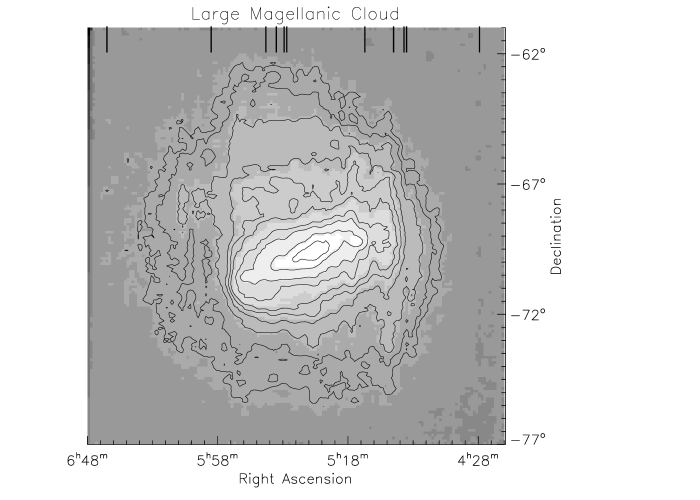
Figure 6: Density map towards the LMC per $0.25\times 0.1$ square degrees. Contours are at 1, 10, 25, 50, 75, 100, 150, 200, 300, 400, 500. Ticks on the upper horizontal axis indicate the position of the missing strips. The structure indicate the presence of a bar and spiral arms.

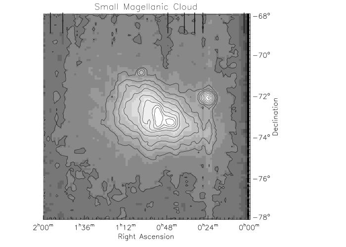
Figure 7: Density map towards the SMC per $0.3\times 0.1$ square degrees. Contours are at 18, 35, 50, 70, 100, 150, 200, 250, 300. Ticks on the upper horizontal axis indicate the position of the missing strips. The concentration of objects on the left side of the SMC structure is due to the galactic globlular cluster 47 Tuc.

Table 6: Detections

$$\begin{array}[]{lrr}\hline\cr\vskip 3.0pt plus 1.0pt minus 1.0pt\cr\mathrm{Wavebands}&\mathrm{SMC}&\mathrm{LMC}\\ \vskip 3.0pt plus 1.0pt minus 1.0pt\cr\hline\cr\vskip 3.0pt plus 1.0pt minus 1.0pt\cr I+J+K_{s}&70000&260000\\ I+J&240000&1050000\\ J+K_{s}&800&1800\\ I+K_{s}&2300&8000\\ \vskip 3.0pt plus 1.0pt minus 1.0pt\cr\hline\cr\end{array}$$

5.1 Nomenclature

5.1.1 Data table (table 7)

The star name is composed by the acronym DCMC (DENIS Catalogue of the Magellanic Clouds) and by the coordinates of the source at the epoch 2000 (Columns 1 and 2) following the IAU convention ‘(Dubois et al. dub (1994)). For example, a star with $(\alpha,\delta)=(1^{h}25^{m}20.15^{s},-73\degr 30\arcmin 15.67\arcsec)$ would have the designation DCMC $J012520.15-733015.6$; right ascension is truncated at the second decimal and the declination at the first. Columns 3, 4, 5, 6, 7 and 8 give the right ascension ($h$, $m$, $s$) and the declination ($\degr$, $\arcmin$, $\arcsec$) at the epoch J2000. Column 9 gives the positional error, i.e. the statistical error calculated during the data processing. Columns 10 and 11 give the pixel coordinates in the corresponding image (Column 12) of the corresponding strip (Column 13), in the $I$ band, where the source is detected. The same quantities are given in Columns 18, 19, 20 and 21 for the $J$ band and in Columns 26, 27, 28 and 29 for the $K_{s}$ band. Columns 14, 22 and 30 give the source magnitudes and Columns 15, 23 and 31 give the associated statistical errors in the $I$, $J$ and $K_{s}$ bands, respectively. Columns 16, 24 and 32 give the extraction flag (table 2) in the three wave bands. Columns 17, 25 and 33 give the image flag (table 1) in the three wave bands. Columns 34 and 35 give the $B$ and $R$ magnitudes from the cross-identification with the USNO–A2.0 catalogue.

5.1.2 Strip quality table (table 8)

Column 1 gives the strip number. Column 2 gives the date of observation of the given strip. Columns 3 and 4 give the nightly zero–point and its standard deviation for the $I$ band. The same quantities are given in Columns 5 and 6 for the $J$ band and in Columns 7 and 8 for the $K_{s}$ band. Column 9 notes information peculiar to the strip in question, for example the photometric shift (Sect. $3.2.3$).

Table 7: Data table: detected sources

$$\begin{array}[]{rlll}\hline\cr\vskip 3.0pt plus 1.0pt minus 1.0pt\cr\mathrm{Col.}&\mathrm{Name}&\mathrm{Description}&\mathrm{Unit}\\ \vskip 3.0pt plus 1.0pt minus 1.0pt\cr\hline\cr\vskip 3.0pt plus 1.0pt minus 1.0pt\cr 1&\mathrm{Origin}&\mathrm{DCMC}&\\ 2&\mathrm{Sequence}&\mathrm{JHHMMSS.ss}\pm\mathrm{DDMMSS.s}\\ 3,4,5&\mathrm{Ra}&\mathrm{Right\,Ascension\,at\,the\,epoch\,2000}&[h,m,s]\\ 6,7,8&\mathrm{Dec}&\mathrm{Declination\,at\,the\,epoch\,2000}&[\degr,\arcmin,\arcsec]\\ 9&\mathrm{RMS-SYS}&\mathrm{Systematic\,postional\,error}&[\arcsec]\\ 10&\mathrm{Xpos-}I&\mathrm{Object\,position\,along\,x}&[pixel]\\ 11&\mathrm{Ypos-}I&\mathrm{Object\,position\,along\,y}&[pixel]\\ 12&\mathrm{FIELD-POS-}I&\mathrm{Reference\,number\,to\,field\,parameters}&\\ 13&\mathrm{STRIP-}I&\mathrm{The\,strip\,number}&\\ 14&\mathrm{MAG-APER-}I&\mathrm{Magnitude\,derived\,within\,}7\arcsec&[mag]\\ 15&\mathrm{MAGERR-APER-}I&\mathrm{Magnitude\,error\,derived\,from\,photon\,statistics\,within\,}7\arcsec&[mag]\\ 16&\mathrm{EXTR-Flag-}I&\mathrm{Extraction\,Flags}&\\ 17&\mathrm{IMA-Flag-}I&\mathrm{FLAG-image\,flags\,OR^{\prime}ed\,over\,the\,iso\,profile}&\\ 18&\mathrm{Xpos-}J&\mathrm{Object\,position\,along\,x}&[pixel]\\ 19&\mathrm{Ypos-}J&\mathrm{Object\,position\,along\,y}&[pixel]\\ 20&\mathrm{FIELD-POS-}J&\mathrm{Reference\,number\,to\,field\,parameters}&\\ 21&\mathrm{STRIP-}J&\mathrm{The\,strip\,number}&\\ 22&\mathrm{MAG-APER-}J&\mathrm{Magnitude\,derived\,within\,}7\arcsec&[mag]\\ 23&\mathrm{MAGERR-APER-}J&\mathrm{Magnitude\,error\,derived\,from\,photon\,statistics\,within\,}7\arcsec&[mag]\\ 24&\mathrm{EXTR-Flag-}J&\mathrm{Extraction\,Flags}&\\ 25&\mathrm{IMA-Flag-}J&\mathrm{FLAG-image\,flags\,OR^{\prime}ed\,over\,the\,iso\,profile}&\\ 26&\mathrm{Xpos-}K&\mathrm{Object\,position\,along\,x}&[pixel]\\ 27&\mathrm{Ypos-}K&\mathrm{Object\,position\,along\,y}&[pixel]\\ 28&\mathrm{FIELD-POS-}K&\mathrm{Reference\,number\,to\,field\,parameters}&\\ 29&\mathrm{STRIP-}K&\mathrm{The\,strip\,number}&\\ 30&\mathrm{MAG-APER-}K&\mathrm{Magnitude\,derived\,within\,}7\arcsec&[mag]\\ 31&\mathrm{MAGERR-APER-}K&\mathrm{Magnitude\,error\,derived\,from\,photon\,statistics\,within\,}7\arcsec&[mag]\\ 32&\mathrm{EXTR-Flag-}K&\mathrm{Extraction\,Flags}&\\ 33&\mathrm{IMA-Flag-}K&\mathrm{FLAG-image\,flags\,OR^{\prime}ed\,over\,the\,iso\,profile}&\\ 34&B\mathrm{PMM}&\mathrm{Blue\,magnitude\,from\,the\,PMM\,catalogue}&\\ 35&R\mathrm{PMM}&\mathrm{Red\,magnitude\,from\,the\,PMM\,catalogue}&\\ \vskip 3.0pt plus 1.0pt minus 1.0pt\cr\hline\cr\end{array}$$

Table 8: Quality table

$$\begin{array}[]{clll}\hline\cr\vskip 3.0pt plus 1.0pt minus 1.0pt\cr\mathrm{Col.}&\mathrm{Name}&\mathrm{Unit}\\ \vskip 3.0pt plus 1.0pt minus 1.0pt\cr\hline\cr\vskip 3.0pt plus 1.0pt minus 1.0pt\cr 1&\mathrm{Strip\,Number}&\\ 2&\mathrm{Observing\,date}&\\ 3&I_{0}&\mathrm{[mag]}\\ 4&\delta_{I_{0}}&\mathrm{[mag]}\\ 5&J_{0}&\mathrm{[mag]}\\ 6&\delta_{J_{0}}&\mathrm{[mag]}\\ 7&K_{0}&\mathrm{[mag]}\\ 8&\delta_{K_{0}}&\mathrm{[mag]}\\ 9&\mathrm{Notes}&\\ \vskip 3.0pt plus 1.0pt minus 1.0pt\cr\hline\cr\end{array}$$

5.1.3 Access

The DENIS Point Source Catalogue towards the Magellanic Clouds, data (table 7) and quality (table 8) tables, are electronically available from CDS via http://cdsweb.u-strasbg.fr/denis.html.

6 Concluding remarks

The catalogue is a suitable tool for the study of late–type stars in the Magellanic Clouds. These studies may involve the statistical separation of various species of stars, i.e. RGB and AGB (both O–rich and C–rich); the characterization of the mass loss properties of these stars, when combined with measurements in the mid and far–IR; the relations of infrared colours and magnitudes with variability, when combined with measurements of light curves (EROS, MACHO) or comparable photometric data (2MASS); the interpretation of the Hertzsprung–Russel diagram through theoretical evolutionary models; the investigation of metallicity effects inside the Magellanic Clouds and in comparison with our own Galaxy; the study of the history of star formation.

- (1) Bertin E., Arnouts S., 1996, A&AS 117, 393
- (2) Bessel M.S., Brett J., 1988, PASP 100, 1134
- (3) Blanco V.M., McCarthy M.F., Blanco B.M., 1980, ApJ 242, 938
- (4) Blanco V.M., McCarthy M.F., 1990, AJ 100, 674
- (5) Borsenberger J., 1997, In: The Impact of Large Scale Near–IR Sky Surveys ASSL 210, Eds F. Garzón, N. Epchtein, A. Omont, W.B. Burton, P. Persi, Kluwer Ac. Publishers, Dordrecht, p. 181
- (6) Carter B.S., 1990, MNRAS 242, 1
- (7) Carter B.S., Meadows V.S., 1995, MNRAS 276, 734
- (8) Cioni M-R., Habing H.J., Loup C., et al., 1998, In: The Stellar Content of Local Group Galaxies, IAU Symp. 192, p. 72
- (9) Costa E., Frogel J.A., 1996, AJ 112, 2607
- (10) Dubois P., Warren W.H., Mead J.M., Lortet M.-C., Dickel H.R., 1994, A&A 281, A12
- (11) Hawarden C., 1992, JCMT-UKIRT, Newsletter 4, 33
- (12) Epchtein N., De Batz B., Capoani L., et al., 1997, The Messenger 87, 27
- (13) Epchtein N., Deul D., Derriere S., et al., 1999, A&A 349, 236
- (14) Fouqué P., Chevallier L., Cohen M., et al., P., 2000, A&AS 141, 313
- (15) Frogel J.A., Blanco V.M., 1983, AJ 274, L57
- (16) Graham J.A., 1982, PASP 94, 244
- (17) Guglielmo F., Deul E.R., Fouqué P., et al., 1996, In: The Impact of Large Scale Near–IR Sky Surveys ASSL 210, Eds F. Garzón, N. Epchtein, A. Omont, W.B. Burton, P. Persi, Kluwer Ac. Publishers, Dordrecht, p. 201
- (18) Hughes S.M.G., 1989, AJ 97, 1634
- (19) Hughes S.M.G., Wood P.R., 1990, AJ 99, 784
- (20) Landolt A.U., 1992, AJ 104 (1), 340
- (21) Loup C., 1998, In: New Views of the Magellanic Clouds, IAU Symp. 190, p. 35
- (22) Menzies J.W., Cousins A.W.J., Benfield R.M., Loing J.D., 1989, SAAO Circ. 13, 1
- (23) Monet D., 1998, AAS 193, 120.03M
- (24) Rebeirot E., Martin N., Mianes P.,Prévot, L., Robin, A. Rousseau J., Peyrin Y., 1983, A&ASS 51, 277
- (25) Rebeirot E., Azzopardi M., Westerlund B.E., 1993, A&AS 97, 3, 603
- (26) Ruphy S., Epchtein N., Cohen M., et al., 1997 A&A 326,597
- (27) Sanduleak N., Philip A.G.D., 1977, Pub. Warner and Swasey Obs., 2, No 5
- (28) Stobie R.S., Gilmore G., Reid N., 1985 A&AS 60, 495
- (29) Westerlund B.E., 1960, Uppsala Astron. Obs. Ann., 4, part no 7, 1
- (30) Westerlund B.E., 1961, Uppsala Astron. Obs. Ann., 5, 2
- (31) Westerlund B.E., 1997, In: The Magellanic Clouds, Cambridge University Press
- (32) Westerlund B.E., Olander N., Richer A.B., Crabtree D.R., 1978, A&AS 31, 61
- (33) Westerlund B.E., Olander N., Hedin B., 1981, A&AS 43, 267