Large Scale Structure in the weakly non-linear regime

Abstract

Is gravitational growth responsible for the observed large scale structure in the universe? Do we need non-gaussian initial conditions or non-gravitational physics to explain the large scale features traced by galaxy surveys? I will briefly revise the basic ideas of non-linear perturbation theory (PT) as a tool to understand structure formation, in particular through the study of higher order statistics, like the skewness and the 3-point function. Contrary to what happens with the second order statistics (the variance or power-spectrum), this test of gravitational instability is independent of the overall amplitude of fluctuations and of cosmic evolution, so that it does not require comparing the clustering at different redshifts. Predictions from weakly non-linear PT have been compared with observations to place constraints on our assumptions about structure formation, the initial conditions and how galaxies trace the mass.

INAOE, Astrofisica, Apdo Postal 216 y 51, 7200, Puebla, Mexico
IEEC/CSIC, Gran Capitán 2-4, 08034 Barcelona, Spain

1. Introduction

Where does structure in the Universe come from? The current paradigm is that it comes from gravitational growth of some small initial fluctuations. The self-gravity of an initial overdensed region increases its density contrast so that eventually the region collapses. For a flat Universe in the linear regime, the local density contrast $\delta\equiv\rho/\bar{\rho}-1$ grows as the expansion factor, eg $D=a$, so that since decoupling linear gravitational growth has the potential of amplifying fluctuations by at least a factor of a thousand. But Gravity is not linear and when objects start collapsing the growth could be much larger. On galactic scales one also has to consider other forces such as hydrodynamics, heating and cooling by friction, dissipation, feedback mechanism from stars, such as nova and supernova explosions, interaction with the CMB and so on.

To test if the above picture of gravitational growth is correct we need to deal with a classical initial condition problem. Because gravitational time scales are very slow, we have no way to measure the growth of individual large scale structures and we need to resort to the statistical study of mean quantities. One can imagine, for example, measuring the rms fluctuations (at a given scale) at different cosmic times to see if this agrees with the predicted amount of gravitational growth, $D$. Observationally this corresponds to finding the clustering properties of some tracer of structure (eg galaxies) at different redshifts. If the tracer is not perfect, we will have some statistical biasing. The problem with this approach is that by the time the rms fluctuations change significantly there typically has also been a substantial cosmic evolution of the corresponding tracers. Thus, it is difficult to disentangle the effects of the underlying cosmological model (which sets the rate $D$ of gravitational growth) from galaxy evolution.

It is therefore important to have a way of testing the gravitational growth paradigm at a single cosmic time or redshift. Higher order correlations and weakly non-linear clustering allows us to do just this. This is because one can construct ratios of higher order correlations to powers of the two point amplitude which are independent of cosmic time or cosmological parameters, but still contain information of the underlying dynamics.

2. Gravitational Growth in the weakly non-linear regime

Gravitational growth increases the density contrast of initially small fluctuations so that eventually the region collapses. The details of this collapse depends on the initial density profile. As an illustration we will focus in the spherically symmetric case. Thus we will study structure growth in the context of matter domination, the fluid limit and the shear-free or spherical collapse approximation. These turns out to be very good approximation for the one-point cumulants of the density fluctuations. It is then easy to find (see Peebles 1980, Gaztañaga & Lobo 2000) the following second order differential equation for the density contrast $\delta$ in the Einstein-deSitter universe ($\Omega_{k}=\Omega_{\Lambda}=0$), eg $a(t)=(t/t_{0})^{2/3}$:

$${d^{2}\delta\over{d^{2}\eta}}+{1\over{2}}~{}{d\delta\over{d\eta}}-{3\over{2}}~{}\delta={4\over{3}}\,{1\over 1+\delta}\,\left({d\delta\over{d\eta}}\right)^{2}~{}+~{}{3\over{2}}~{}\delta^{2}$$

where we have shifted to the rhs all non-linear terms, and used the $\eta\equiv\ln(a)$ as our time variable. This equation reproduces the equation of the spherical collapse model (SC). As one would expect, this yields a local evolution so that the evolved field at a point is just given by a (non-linear) transformation of the initial field at the same point, with independence of the surroundings. The linear solution factorizes the spatial and temporal part:

$$\delta_{l}(\hbox{\twelveBF x},t)=\,D(t-t_{0})\,\delta(\hbox{\twelveBF x},t_{0})=\,D(t)\,\delta_{0}(\hbox{\twelveBF x})$$

where $D$ is the linear growth factor, which from the above differential equation:

$$D(t)=C_{1}~{}e^{\eta}~{}+~{}C_{2}~{}e^{-3/2\eta}=C_{1}~{}a(t)~{}+~{}C_{2}~{}a(t)^{-3/2}$$

with growing $D\sim a$ and the decaying $D\sim a^{-3/2}$ modes. Thus, the initial fluctuations, no matter of what amplitude, grow by the same factor, $D$, and the statistical properties of the initial field are just linearly scaled. For example the linear rms fluctuations $\sigma_{l}$ or its variance $\sigma^{2}_{l}$ gives:

$$\sigma^{2}_{l}~{}\equiv~{}\overline{\xi}_{2}~{}\equiv~{}\mathop{\bigl{\langle}}\delta^{2}(t)\mathop{\bigr{\rangle}}=\mathop{\bigl{\langle}}D(t-t_{0})^{2}\delta_{0}^{2}\mathop{\bigr{\rangle}}=D(t-t_{0})^{2}~{}\sigma_{0}^{2}$$

where $\delta_{0}=\delta(t_{0})$ and $\sigma_{0}$ refer to some initial reference time $t_{0}$: $\sigma_{0}^{2}\equiv<\delta_{0}^{2}>$.

We are interested in the perturbative regime ($\delta\rightarrow 0$), which is the relevant one for the description of structure formation on large scales. The non-linear solution for $\delta$ can then be expressed directly in terms of the linear one, $\delta_{l}$:

$$\delta=f(\delta_{l})=\,\sum_{n=1}^{\infty}~{}{\nu_{n}\over n!}\,~{}{[\delta_{l}]^{n}}$$

Thus all non-linear information is encoded in the $\nu_{n}$ coefficients. We can now introduce this expansion in our non-linear differential equation, with $\delta_{l}$ given by the linear growth factor $D=a=e^{\eta}$, and compare order by order to find:

$$\nu_{2}={34\over 21}~{}~{}~{};~{}~{}~{}\nu_{3}={682\over 189}~{}~{}~{};~{}~{}~{}\nu_{4}={446440\over 43659}~{}~{}~{};~{}~{}~{}\nu_{5}={8546480\over 243243}~{}~{}~{}~{}~{}~{}\dots$$

These results are derived for the Einstein-de Sitter, but are also a good approximation for other cosmologies (eg Bouchet et al. 1992, Bernardeau 1994a, Fosalba & Gaztañaga 1998b, Kamionkowski & Buchalter 1999). For non-standard cosmologies or a different equation of state see Gaztañaga & Lobo (2000).

One can now find the N-order cumulants $\overline{\xi}_{N}\equiv\mathop{\bigl{\langle}}\delta^{N}\mathop{\bigr{\rangle}_{c}}{}$, where $N=2$ corresponds to the variance. Here the expectation values $\mathop{\bigl{\langle}}...\mathop{\bigr{\rangle}}$ correspond to an average over realizations of the initial field. On comparing with observations we assume the fair sample hypothesis (§30 Peebles 1980), by which we can commute spatial integrals with expectation values. Thus, in practice $\mathop{\bigl{\langle}}...\mathop{\bigr{\rangle}}$ is the average over positions in the survey area. It is useful to introduce the N-order hierarchical coefficients: $S_{N}\,=\overline{\xi}_{N}/\overline{\xi}_{2}^{N-1}$, eg skewness for $S_{3}$ and kurtosis for $S_{4}$. These can easily be estimated from the series expansion above by just taking expectation values of different powers of $\delta$ (eg see Fosalba & Gaztañaga 1998a). For leading order Gaussian initial conditions we have:

$$S_{3}=3~{}\nu_{2}~{}~{}~{};~{}~{}~{}S_{4}=4~{}\nu_{3}+12~{}\nu_{2}^{2}~{}~{}~{};~{}~{}~{}S_{5}=5~{}\nu_{4}+60~{}\nu_{3}\nu_{2}+60~{}\nu_{2}^{3}$$

These results have also been extended to the non-Gaussian case, see Fry & Scherrer (1994) Chodorowski & Bouchet (1996), Gaztañaga & Mahonen (1996), Gaztañaga & Fosalba (1998). If we take for $\nu_{2}$ the non-linear solution above, eg $\nu_{2}=34/21$, the skewness yields $S_{3}=3\nu_{2}=34/7$, which reproduces the exact perturbation theory (PT) result by Peebles (1980). Thus the above (SC) model gives the exact leading order result for the skewness. This is also true for higher orders (see Bernardeau 1992 and Fosalba & Gaztañaga 1998a). These expressions have to be corrected for smoothing effects (see Juszkiewicz et al. 1993, Bernardeau 1994a, 1994b, and Fosalba & Gaztañaga 1998a) and possibly from redshift space distortions (eg Hivon et al 1995, Scoccimarro, Couchman and Frieman 1999). Next to leading order terms have been estimated by Scoccimarro & Frieman (1996), Fosalba & Gaztañaga (1998a,b).

The 1-point cumulants measured in galaxy catalogues have been compared with these PT predictions (eg Bouchet et al. 1993, Gaztañaga 1992, Gaztañaga & Frieman 1994, Baugh, Gaztañaga & Efstathiou 1995, Baugh & Gaztañaga 1996, Colombi etal 1997, Hui & Gaztañaga 1999). The left panel of Figure 1 shows a comparison of $S_{N}$ measure in the APM Galaxy Survey (Maddox et al. 1990), with the predictions above (see Gaztañaga 1994, 1995 for more details). The agreement between predictions (lines) and measurements (points) on scales $R>10h^{-1}\,\mbox{Mpc}$ (where $\overline{\xi}_{2}<1$), is quite good indicating that the APM galaxies follow the non-linear gravitational growth picture. For errors on statistics see Szapudi, Colombi and Bernardeau (1999) and references therein.

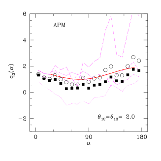
Figure 1.: Figures in the left panel show estimates of $S_{N}$, for $N=3-6$, from the APM galaxy catalogue. Lines correspond to the PT predictions. Figures in the right panel shows the APM projected 3-point amplitude $q_{3}(\alpha)$, for triplets of objects $1,2,3$ on the sky at fixed $\theta_{12}=\theta_{13}=2$ deg and as a function of $\alpha$ the interior angle between these two triangle sides. The thick line shows the PT predictions.

2.1. Biasing: tracing the mass

The expressions above apply to unbiased tracers of the density field; since galaxies of different morphologies are known to have different clustering properties, at least some galaxy species are biased. As an example, suppose the probability of forming a luminous galaxy depends only on the underlying mean density field in its immediate vicinity. The relation between the density field as traced by galaxies $\delta_{gal}(\hbox{\twelveBF x})$ and the mass density field $\delta(\hbox{\twelveBF x})$, can then be written as:

$$\delta_{gal}(\hbox{\twelveBF x})=f(\delta(\hbox{\twelveBF x}))=\sum_{n}~{}{b_{n}\over{n!}}~{}~{}\delta^{n}(\hbox{\twelveBF x}),$$

where $b_{n}$ are the bias parameters. Thus, note how biasing and gravity could produce comparable non-linear effects. To leading order in $\overline{\xi}_{2}$, this local bias scheme implies $\overline{\xi}_{2}^{gal}=b_{1}^{2}\overline{\xi}_{2}$ and (see Fry & Gaztañaga 1993):

$$S_{3}^{gal}={S_{3}\over{b_{1}}}+3~{}{b_{2}\over{b^{2}_{1}}}~{}~{}~{};~{}~{}~{}S_{4}^{gal}={S_{4}\over{b_{1}^{2}}}+12~{}{b_{2}S_{3}\over b_{1}^{3}}+4~{}{b_{3}\over b_{1}^{4}}+12~{}{b_{2}^{2}\over b_{1}^{4}}~{}~{}~{};~{}~{}~{}\dots$$

Gaztañaga & Frieman (1994) have used the comparison of $S_{3}$ and $S_{4}$ in PT with the corresponding measured APM values (as shown in Figure 1) to infer that $b_{1}\simeq 1$, $b_{2}\simeq 0$ and $b_{3}\simeq 0$, but the results are degenerate due to the relative scale-independence of $S_{N}$ and the increasing number of biasing parameters. One could break this degeneracy by using the configuration-dependence of the projected 3-point function, $q_{3}(\alpha)$, as proposed by Frieman & Gaztañaga (1994), Fry (1994), Matarrese, Verde & Heavens (1997) Scoccimarro et al (1998). As shown in Frieman & Gaztañaga (1999), the configuration-dependence of $q_{3}({\alpha})$ on large scales in the APM catalog is quite close to that expected in perturbation theory , suggesting again that $b_{1}$ is of order unity (and $b_{2}\simeq 0$) for these galaxies. This is illustrated in the right panel of Figure 1. The solid curves show the predictions of weakly non-linear gravitational growth. The APM galaxy measurements are shown as symbols ; other curves show results for each of the zones. The agreement indicates that large-scale structure is driven by non-linear gravitational instability and that APM galaxies are relatively unbiased tracers of the mass on these large scales.

3. Conclusions

The values of $S_{N}=\overline{\xi}_{N}/\overline{\xi}_{2}^{N-1}$ can be measured as traced by the large scale galaxy distribution (eg Bouchet et al. 1993, Gaztañaga 1992, 1994, Szapudi el at 1995, Hui & Gaztañaga 1999 and references therein), and also the weak-lensing (Bernardeau et al. 1997, Gaztañaga & Bernardeau 1998) or the Ly-alpha QSO absorptions (Gaztañaga & Croft 1999). These measurements of the skewness $S_{3}$, kurtosis $S_{4}$, and so on, can be compared with the predictions from weakly non-linear perturbation theory (see Figure 1) to place constraints on our assumptions about gravitational growth, initial conditions or biasing at a given redshift (see Mo, Jing & White 1997). Contrary to what happens with the second order statistics (eg the variance), this test of gravitational instability is quite independent of the overall amplitude of fluctuations and other assumptions of our model for cosmological evolution, and does not require comparing the clustering at different redshifts. As shown in Gaztañaga & Lobo (2000), one can also use the $S_{N}$ measurements to constraint non-standard cosmologies.

Frieman & Gaztañaga (1999) have presented new results for the angular 3-point galaxy correlation function in the APM Galaxy Survey and its comparison with theoretical expectations (see also Fry 1984, Scoccimarro et al. 1998, Buchalter, Jaffe & Kamionkowski 2000). For the first time, these measurements extend to sufficiently large scales to probe the weakly non-linear regime (see previous work by Groth & Peebles 1977, Fry & Peebles 1978, Fry & Seldner 1982). On large scales, the results are in good agreement with the predictions of non-linear perturbation theory, for a model with initially Gaussian fluctuations (see Figure 1). This reinforce the conclusion that large-scale structure is driven by non-linear gravitational instability and that APM galaxies are relatively unbiased tracers of the mass on large scales; they also provide stringent constraints upon models with non-Gaussian initial conditions (eg see Gaztañaga & Mahonen 1996; Peebles 1999a,b; White 1999; Scoccimarro 2000).

References

Baugh, C.M., & Gaztañaga, E. 1996, MNRAS, 280, L37

Baugh, C.M., Gaztañaga, E., Efstathiou, G., 1995, MNRAS, 274, 1049

Bernardeau, F., 1992, ApJ 392, 1

Bernardeau, F., 1994a, A&A 291, 697

Bernardeau, F., 1994b, AJ433, 1

Bernardeau, F.,van Waerbeke, L., Mellier, Y. 1997, A&A 322, 1

Bouchet, F. R., Juszkiewicz, R., Colombi, S., & Pellat, R. 1992, ApJ,394,L5

Bouchet, F. R., Strauss, M. A., Davis, M., Fisher, K. B., Yahil, A., & Huchra, J. P., 1993, ApJ 417, 36

Buchalter, A., Jaffe, A., Kamionkowski, M., 2000, ApJ, 530, 36

Colombi, S., Bernardeau, F., Bouchet, F. R., Hernquist, L., 1997, MNRAS, 287, 241.

Chodorowski, M. & Bouchet, F. 1996, MNRAS, 279, 557

Fosalba, P. & Gaztañaga, E., 1998a, MNRAS 301, 503

Fosalba, P. & Gaztañaga, E., 1998b, MNRAS 301, 535

Frieman, J. A., & Gaztañaga, E. 1994, ApJ,425, 392

Frieman, J. A., & Gaztañaga, E. 1999, ApJ Lett, 521, L83

Fry, J. N. 1984, ApJ, 279, 499

Fry, J. N. 1994, Phy. Rev. Lett. 73, 215

Fry, J. N. & Gaztañaga, E. 1993, ApJ, 413, 447

Fry, J. N. & Peebles 1978, ApJ, 221, 19

Fry, J. N. & Seldner, M. 1982, ApJ, 259, 474

Fry, J. N. & Scherrer, R. 1994, ApJ, 429, 36

Gaztañaga, E. 1992, ApJ Lett, 398, L17

Gaztañaga, E. 1994, MNRAS, 268, 913

Gaztañaga, E. 1995, MNRAS, 454, 561

Gaztañaga, E. & Bernardeau, F. 1998, A & A, 331, 829

Gaztañaga, E. & Croft, R.A.C., MNRAS, 309, 885

Gaztañaga, E. & Fosalba, P., 1998, MNRAS, 301, 524

Gaztañaga, E. & Frieman, J. A., 1994, ApJ, 437, L13

Gaztañaga, E. & Lobo, A., 2000, astro-ph/0003129

Gaztañaga, E. & Mahonen, P. 1996, ApJ, 462, L1

Groth, E. J. & Peebles, P. J. E. 1977, ApJ, 217, 385

Hivon, E., Bouchet, F. R., Colombi, S. & Juszkiewicz, R., 1995, A&A, 298, 643

Hui, L. & Gaztañaga, E. 1999, ApJ, ApJ, 519, 1

Juszkiewicz, R., Bouchet, F., & Colombi, S. 1993, ApJ, 412, L9

Kamionkowski, M. & Buchalter, A. 1999, ApJ, 514, 7

Maddox, S.J., Efstathiou, G., Sutherland, W.J., Loveday, J. 1990, MNRAS, 242, 43P

Matarrese, S., Verde, L., Heavens, A. F., 1997, MNRAS 290, 651

Mo, H.J., Jing, Y.P., White, S.D.M., 1997, MNRAS 284, 189

Peebles, P. J. E. 1980, The Large Scale Structure of the Universe, Princeton: Princeton University Press

Peebles, P. J. E. 1999a, ApJ 510, 523

Peebles, P. J. E. 1999b, ApJ 510, 531

Scoccimarro, R, 2000, astro-ph/0002037

Scoccimarro, R. & Frieman, J., 1996, ApJ Supp, 105, 37

Scoccimarro, R., Couchman, H. M. P., & Frieman, J., 1999, ApJ, 517, 531

Scoccimarro, R., Colombi, S., Fry, J. N., Frieman, J., Hivon, E., & Melott, A. 1998, ApJ, 496, 586

Szapudi, I., Dalton, G.B., Efstathiou, G. & Szalay, A. S. 1995, ApJ, 444, 520

Szapudi, I., Colombi, S., Bernardeau, F., 1999, MNRAS, 310, 428

White, M., 1999, MNRAS 310, 511