On mesogranulation, network formation and supergranulation

Abstract

We present arguments which show that in all likelihood mesogranulation is not a true scale of solar convection but the combination of the effects of both highly energetic granules, which give birth to strong positive divergences (SPDs) among which we find exploders, and averaging effects of data processing. The important role played by SPDs in horizontal velocity fields appears in the spectra of these fields where the scale $\sim$4 Mm is most energetic; we illustrate the effect of averaging with a one-dimensional toy model which shows how two independent non-moving (but evolving) structures can be transformed into a single moving structure when time and space resolution are degraded.

The role of SPDs in the formation of the photospheric network is shown by computing the advection of floating corks by the granular flow. The coincidence of the network bright points distribution and that of the corks is remarkable. We conclude with the possibility that supergranulation is not a proper scale of convection but the result of a large-scale instability of the granular flow, which manifests itself through a correlation of the flows generated by SPDs.

1 Introduction

In the traditional view of solar convection seen at the sun’s surface, three scales play the main roles: granulation (1 Mm) which shows up as an intensity pattern most probably first seen by Herschel in 1801 BLD84, supergranulation ($15-30$ Mm) which appears in (but not only) dopplergrams of the full disk of the sun as a pattern of horizontal velocities and which was first noticed by HartHart56b and confirmed by Leighton et al. LNS62, and mesogranulation ($3-10$ Mm) observed by November et al. NTGS81 on Doppler measurements of vertical velocities.

While the dynamics of granulation is rather well understood, its scale being controlled by the balance of radiative diffusion of heat and convection, the origin of the two other scales remains largely mysterious. The ionization of helium was often invoked to explain these two scales since the first and second ionizations of this atom occur at depths similar to the mesogranular and supergranular scale respectively. However, this geometrical explanation is based on a “laminar view” of solar convection which is, on the contrary, very strongly turbulent.

The aim of the present paper is to investigate the dynamics of scales larger than that of the granulation, using the horizontal flows given by granular motions determined by the new algorithms described in Roudier et al. (1999). Briefly, these algorithms, Local Correlation Tracking on binarized images (LCT_bin) or Coherent Structure Tracking (CST), allow us to increase noticeably the spatial and temporal resolutions of the surface velocity fields; typically, we can bring the spatial grid size down to 0″7 and the time step down to 5 mn.

Thus, we first concentrate on mesogranulation (Sect. 2) and show the major role played at this scale by strong positive divergences (SPDs) and by averaging procedures. It turns out, indeed, that what has been described in previous work as mesogranulation results from a combination of a physical phenomenon (SPDs among which are found exploding granules) and a data processing effect applied to a turbulent flow (averaging). Since each author had his own technique for averaging data, results have been rather confusing and no clear-cut description of mesogranulation has emerged. We show here that when averaging is properly controlled, no quasi-steady flow can be detected in the mesoscale range.

We then proceed (Sect. 3) with the investigation of the transport properties of the mesoscale flows and show that the supergranulation scale appears when the positions of concentrations of corks are compared to the positions of network bright points. We conclude the paper with a discussion of a model which seems to explain many of the observations and the interactions of the three scales.

2 Mesogranulation

Since its discovery by November et al. NTGS81, mesogranulation has been sought using many different techniques (Doppler measurements, intensity variations, horizontal velocity fields and their divergence) with the idea that one could exhibit a quasi-steady cellular motion as clearly as granulation. However, the reports of observations aimed at pointing out this new feature of solar convection have never been clear-cut and always difficult to compare to each other.

In Table LABEL:meso_table we summarize all the previous studies on mesogranulation. A common result of these studies is that they always find some features in the mesogranulation range of scales, i.e. within length scales between 4″ and 12″ (or 3 Mm and 10 Mm) and on time scales between 30 mn and 6 h. The features are patterns either in intensity, or in radial velocity, or in horizontal divergence, for example. The picture left by mesogranulation observations is therefore fuzzy: neither its characteristic size or time is well established and vary from one author to another.

Figure 1: Power spectra $E_{\tau}(k)$ of the horizontal velocity fields using the three hour data set of Pic du Midi. The grid size is 0″7 (1″= 728 km); note that the field of view is 58.2″$\times$47.6″. All the spectra have been normalized by their maximum value. The different line styles refer to the time-averaging window of size $\tau$.

Figure 2: Linear correlation of successive time-averaged velocity fields. For each averaging window we computed the correlation of both the $x$- and $y$- components of the velocity field.

2.1 Spectra and correlations

In order to better understand the situation, it is useful to consider the physics which leads to the above mentioned observations. This is obviously turbulent convection: motions seen at the sun’s surface result from the superposition of a large number of scales constituting the turbulent spectrum. The relevant questions are therefore: why should a scale like mesogranulation single out among other scales? And if it does, how would we recognize and characterize it?

Concerning granulation, the answers are known: it is the balance between radiative diffusion and advection which determines the size of granules and it emerges from other scales as the one with the highest contrast in intensity and with the largest fluctuations of velocity. The spectrum of turbulent kinetic energy shows a maximum around this scale.

Figure 3: First two rows: Time sequence of two structures (Gaussians) emerging at two different places with a slight time-delay. Bottom row: The same structures are now seen after convolution by a time window of width $\Delta t=20$ and a spatial window of width $\Delta x=2.5$; after a local growth, a single structure seems to move and then decays.

At mesoscale, we do not know which mechanism could distinguish any particular scale; we may, however, try to recognize a scale which stands out and therefore search for a peak or a break of the slope in the kinetic energy spectrum. Such a feature in the spectrum is indeed the signature that some physical mechanism is injecting energy at a specific scale.

In previous work EMRN93, spectra of kinetic energy have not shown any characteristic feature at scales larger than granulation. In fact, large-scale features appear in turbulent flows with time averages. Indeed, let us suppose that the kinetic energy spectrum varies as $E(k)\propto k^{-\alpha}$ in the mesoscale range; using dimensional arguments, it turns out that the typical lifetime of structures of wavenumber $k$ is $\tau_{k}\propto k^{(\alpha-3)/2}$ which means that the lifetime of turbulent structures increases with their size since $\alpha<3$. In other words, long time-averages show large-scale features and the longer the average the larger the scale. This point is clearly illustrated in Fig. 1 where we have computed kinetic energy spectra of the horizontal flow derived from granule tracking in Pic du Midi data RRMV99. These spectra $E_{\tau}(k)$ are defined as follows: The mean kinetic energy (defined by a time window of length $\tau$) at one point of the field reads:

$$\frac{1}{2}\left\langle v^{2}\right\rangle_{\tau}=\int_{0}^{\infty}E_{\tau}(k)dk$$

where $E_{\tau}(k)$ is related to the Fourier transform of the velocity components $\tilde{v}_{x}$, $\tilde{v}_{y}$ by

$$E_{\tau}(k)=\int_{0}^{2\pi}\left(|\tilde{v}_{x}|^{2}+|\tilde{v}_{y}|^{2}\right)kd\theta,$$

where $k_{x}=k\cos\theta$ and $k_{y}=k\sin\theta$ are the components of the wave vector. In this figure we clearly see the build-up of large-scales and the disappearance of small scales when the time averaging window is made longer. The average of the spectra of the velocity fields determined by LCT_bin and a 15mn-window clearly shows a peak at a scale of $\sim$5″ (3500 km); this peak is the signature of the most energetic horizontal flows.

Figure 4: Same as Fig. 1 but with a grid size of 1″96.

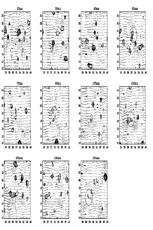
Figure 5: Evolution of the flow field with the contours of high positive divergence overlaid. The four black dots locate the position of mesogranule 5 of Muller et al. MARVSFST92 while the circle emphasizes the position corresponding to the time of the snapshot. In the last snapshot the numbers show the successive position of mesogranule 5. We clearly see from this sequence that no steady state structure of the divergence field moves from position 1 to 4 during the sequence. Axis units are in arcsec.

To further emphasize the turbulent nature of mesoscale features, we compute the correlation between successive time-averaged velocity fields as a function of time; we compute

$$C_{x}=\frac{\overline{\left(\left\langle v_{x}\right\rangle_{\tau}-\overline{\left\langle v_{x}\right\rangle_{\tau}}\right)(t)\left(\left\langle v_{x}\right\rangle_{\tau}-\overline{\left\langle v_{x}\right\rangle_{\tau}}\right)(t+n\tau)}}{\sqrt{\overline{\left(\left\langle v_{x}\right\rangle_{\tau}-\overline{\left\langle v_{x}\right\rangle_{\tau}}\right)^{2}(t)}\overline{\left(\left\langle v_{x}\right\rangle_{\tau}-\overline{\left\langle v_{x}\right\rangle_{\tau}}\right)^{2}(t+n\tau)}}}$$

as a function of $n$ ($t$ is arbitrary); in this expression overbars indicate spatial averages and $\left\langle\cdot\right\rangle_{\tau}$ stands for a time average of length $\tau$. Results are plotted in Fig. 2. They show that the autocorrelation of the mean velocity fields is halved after one time step. This again emphasizes the role played by the time window which selects a spatial structure whose lifetime is precisely of the order of the time window, thus showing that no quasi-steady flow exists on a time scale longer than 15 mn.

2.2 Pitfalls of data processing

Turbulence, however, is not the only difficulty of this problem; data processing may also interfere and contribute to blur the results.

As a first instance, let us compute the kinetic energy spectra of horizontal flows, but using a larger spatial window (than in Fig. 1) for the determination of the velocity field. The result is shown in Fig. 4 for a 2″-resolving window. Very clearly the peak is now shifted to 12″ (8.7 Mm). This emphasizes the high sensitivity of the velocity field patterns (scales) to the choice of the sampling window.

Finally, we would like to mention another effect of data processing which can unduly extend the lifetime of mesoscale features. This is the use of sliding time windows. Indeed, as illustrated in Fig. 3 such windows can transform two independent time-evolving structures into a single moving structure. This is what happened when Muller et al. (1992) described a three-hour-living mesogranule which was used to show the supergranular flow. In fact, as shown by Fig. 5, an independent time sampling shows that no coherent structure lasts such a long time but new structures emerge after $\sim$30 mn.

We therefore interpret the results of previous work on mesogranulation as a consequence of uncontrolled averaging procedures. This explains the large variability of results which have been published on mesogranulation: they are all dependent on the way authors have combined their averages.

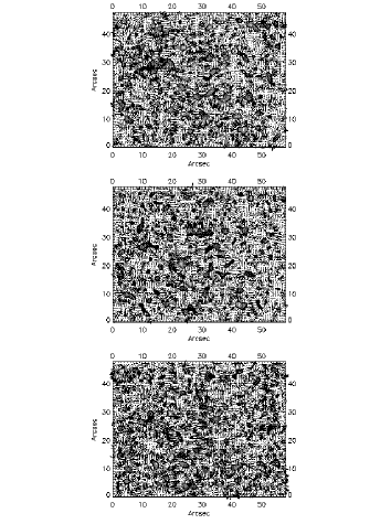
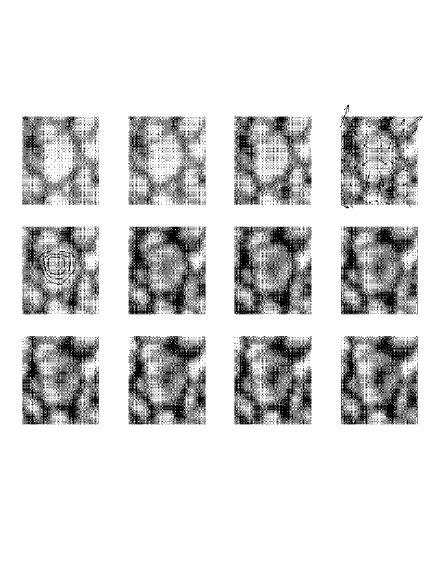
Figure 6: Evolution of the velocity field with the high positive values (thresholded) of divergence overlaid. Each field was computed using a 5 mn time-window with the LCT_bin algorithm (cf Roudier et al. 1999). The time step is 5 mn.

Figure 7: A time sequence of an exploding granule with the corresponding velocity or divergence field overlaid. Each snapshot is 5.6″wide and the time step is 20 s.

Figure 8: A histogram of the lifetime of patterns with positive divergence above a given threshold. The lifetime is defined as the time spent by a (simply connected) pattern over the threshold; the mean lifetime is 15 mn.

2.3 Strong positive divergences (SPDs)

The foregoing results, however, leave unanswered the question of the origin of kinetic energy in the mesoscale range; we may indeed wonder which flow patterns are contributing to the spectral peak at $\sim 5$″ in Fig. 1. A plot of the velocity field along with its divergence (Fig. 7) shows that the strong horizontal flows are generally associated with strong positive divergences (SPDs) among which the exploding granules are the most energetic. This is well illustrated by the two time sequences in Fig. 7 and Fig. 7. From Fig. 7, it is quite clear that the divergence field is highly variable, showing patterns which may extend up to 10″ (7.3 Mm). A histogram of the lifetime of these patterns (Fig. 8) gives a mean lifetime of 15 mn which is short.

Ending this section, we are therefore lead to the conclusion that no specific scale exists in the mesogranulation range except the scale of horizontal flows featured by SPDs. Hence we confirm the conclusion of Straus and Bonaccini SB97 that no gap in the kinematic energy spectrum separates granulation from mesogranulation which therefore must be considered just as the large-scale extension of granulation.

3 Supergranulation

3.1 Mean flows and SPDs

We may now wish to know whether supergranulation plays some part in the motion of granules. A first look at the spectrum of the 3-hour-average velocity field (Fig. 1) shows some energy at $\sim 30$″ (22 Mm). However, this spectral peak is only suggestive since the field of view is just 47.6″. Turning to real space (as opposed to spectral space), a plot of the velocity field (Fig. 9) shows that indeed a large-scale velocity field may exist. The rms velocity of the 3-hour-average field is $\sim 230$ m/s. On the unfiltered field we clearly see the imprint of SPDs with their typical size of 5″; this indicates that the origin of the mean flow may be found in the cumulative effects of SPDs. Furthermore, if this mean field is identified with supergranulation, we have at hand its origin: correlated SPDs.

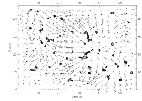
Figure 9: The three hour time average of the velocity field using a 0.7″window (above) and a 2.8″window (below). Contours show the thresholded positive divergence.

3.2 Network formation from measured velocity fields

Figure 10: Top: Corks’ trajectories for the velocity field derived from granule motions in the Pic du Midi data set. Middle: Corks’ distribution after three hours of advection. Bottom: Same as (middle) but with simulated velocity fields (see text).

One way to confirm the view that a three-hour time average of horizontal flows shows the supergranulation scale, is to focus on its transport properties. This technique was already used in the past by Simon and Weiss SW89. It consists of integrating the trajectories of floating corks, initially uniformly distributed, and characterizing their spatial distribution after some time. Simon and Weiss used the SOUP data sequence, which lasted 28 mn, to determine a kinematic model of the horizontal velocity field. Then, they integrated the cork trajectories during a time very much longer (up to 16 h) than the data sequence. Our method is much closer to the data: with the techniques described in Roudier et al. (1999), we determine the velocity field evolution of the Pic du Midi data set with a high spatial and temporal resolution (0″7 and 5 mn). We then use this field to integrate the cork trajectories during the three hours of recorded data.

As shown in Fig. 10, corks are expelled from certain regions, whose size varies between 5 Mm and 15 Mm and again SPDs seem to play a major role. We cannot say that the cells thus formed are “supergranules” since they would continue to evolve if our data set were longer. If the concentration of corks is plotted, however, the supergranulation scale already appears. The clearest evidence of this is given by the remarkable coincidence between the regions with a high density of corks and the positions of network bright points (Fig. 11). This result should be compared with the one of Brandt et al. BRST94 who found a similarity between cork distribution and the Ca-network.

Referring back to the mean divergence field (Fig. 9), we also see that the regions with negative divergence are the ones where corks and network bright points tend to concentrate.

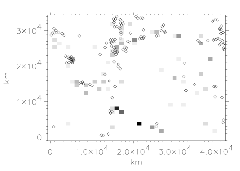
Figure 11: Corks’ density (squares in grey scale) and network bright points in the same field of view; their position are derived from Muller et al. 1992. The distribution shown by the squares represents 70% of the corks, the rest being distributed randomly in the field.

Finally, we also used corks to estimate a horizontal diffusivity $D=<r^{2}\!>/4t$ following Berger et al. BLST98. We found values between 50 km²/s and 100 km²/s but, as this diffusivity did not reach an asymptotic value at the end of our time-sequence, we think that the aforementioned values only show the amplitude of the transport but nothing about its physical origin (advection, diffusion, abnormal or turbulent diffusion).

3.3 Network formation from simulated velocity fields

In order to show the leading role of SPDs, we extracted from the data their positions in space and time as well as their mean radii. We used them to determine the amplitudes ($V_{n}$) of the model flow used by Simon and Weiss (1989) and Simon et al. STW91, namely

$$\@vec{v}=\sum_{n}V_{n}{|\@vec{r}-\@vec{r}_{n}|\over R}\;e^{-|\@vec{r}-\@vec{r}_{n}|^{2}/R^{2}}\@vec{e}_{n}$$

where $\@vec{r}_{n}$ designates the position of SPDs, $R$ their range of influence, which lies between 0.5″ and 3″ with a mean value of 2.3″, and $\@vec{e}_{n}$ the direction of their flow.

Using such a model flow, we have repeated the calculation for the advection of corks and found a distribution very similar to the one obtained when using the full data (see Fig. 10).

It therefore turns out that SPDs give the main contribution to the horizontal transport of passive scalars.

4 Discussion

4.1 Mesoscale flows

The analysis of flow motions at mesoscale that we presented in Sect. 3 has shown that the scale of flow patterns is controlled by the size of the averaging time window. We interpret this result as evidence of the turbulent nature of the kinetic energy spectrum in this range of scales. We therefore refute the idea that some quasi-steady flow exists at mesoscale and show that previous identifications of mesogranules advected by a supergranular flow, as shown by Muller et al. (1992) for instance, are an artefact of the averaging procedure. We identify the only mechanism able to structure the horizontal flow field as being SPDs among which we find exploding granules. However, the scale controlled by SPDs is rather centered around 5″ (3.5 Mm) which is small compared to the scale generally attributed to mesogranulation (5-10 Mm); we conjecture that these latter scales are in fact built up by the nonlinear interactions of the former ones and form the (turbulent) continuation of the granular motion spectrum. Using two-dimensional simulations Ploner Ploner98 also concludes that mesoscale flows can result from nonlinear interactions of granular flows.

We have shown subsequently that the use of Pic du Midi velocity fields in computing trajectories of floating corks, shows that at the end of the time integration, which we take equal to the length of the data set, corks concentrate in regions which coincide with those occupied by network bright points. It thus turns out that in a rather short time the supergranulation scale emerges from the flow delineated by granule motions.

These results show that the traditional view which assumes supergranulation as a quasi-steady horizontal flow driven by the ionization of helium is certainly too simple. Obviously the build-up of the supergranulation scale as far as magnetic flux tubes are concerned, results from a process of turbulent transport in which SPDs play an important part.

4.2 A model for supergranulation

In order to explain the above mentioned observations and some others, we now present a model which seems to square with all the known constraints of supergranulation.

Let us consider the surface convection of the sun as a set of granules. Assume that each granule interacts nonlinearly, mainly with its nearest neighbours. The set of granules behave like a set of nonlinearly coupled oscillators. A general behaviour of such a system is that its energy can be focused on one or very few oscillators whose motion is then very much enhanced DP93. Such oscillators collecting the kinetic energy of the others would appear, in the solar context, as SPDs or even exploders. This may also be seen as a manifestation of intermittency of the turbulent solar flow. Now it has been noticed that such exploding granules appear generally in neighbouring places (see the mean divergences) which means that some temporal and spatial correlations exist between them, namely that a large-scale flow organizes their appearance (or vice-versa). This large-scale flow is obviously supergranulation; its origin should be found in a large-scale instability of the flow expressed by the set of granules.

Recent theoretical work GVF94; SSSF89 on turbulent flows has indeed shown that a large-scale perturbation of some given steady spatially periodic flow can be unstable in some bandwidth of wavenumbers. Typically two kinds of situations may occur: the original small-scale flow is invariant with respect to parity or not. If it is not, large-scale instabilities occur through an AKA effect which is the equivalent of the $\alpha$-effect of turbulent MHD flows; if it is parity invariant, which is the case of solar granulation (flows are hardly helical), then instability appears through a negative eddy viscosity; a range of large-scale modes is then destabilized and some large-scale coherent flow starts. However, this new flow is rapidly hindered by the motions it induces: as the Reynolds stress distribution is modified, usually the turbulent viscosity comes back to positive values; in our case we are considering turbulent convection and any flow increasing the convective heat flux will be slowed by the overcooled material. A similar scenario was also envisaged by Krishan Krish91 using arguments based on inverse cascade of two-dimensional turbulence; indeed, large-scale instabilities are a way of realizing an inverse cascade. However, the mechanism invoked by Krishan is rather close to the AKA-effect which requires helical motions at supergranular scales; such motions do not seem to be observed. On the other hand, higher in the atmosphere, the stratification stabilizes the fluid and may produce two-dimensional motions which can ease energy transfer to large scales.

We therefore understand why large-scale (with respect to granulation scale) flows like supergranulation will appear. We also understand why supergranulation does not realize a perfect pavement of the whole sun as does granulation. The development of the large-scale instability is a stochastic process which results from a given arrangement of the granular flow. It has not the constraint, as any convective flow, to transport heat.

We also understand why the main downflows of a supergranule are not at its boundary as revealed by the MDI instrument on board of SOHO (see http://sohowww.nascom.nasa.gov/gallery/MDI/ mdi009.html,mdi009.ps or Zahn 1999). They are in fact associated with the most energetic granules i.e. the exploders, and therefore occur mainly in the bulk of the supergranule. The downflows on the boundaries should not be very intense since the supergranular flow must remain weak compared to the granular flows.

Hence, this model explains an interesting number of observations. Essentially, it states that supergranular flows are surface flows which do not result from a large-scale thermal instability.

5 Conclusion

To conclude this paper we would like to emphasize the point that the picture of surface solar convection which has been popular in the literature and where supergranulation advects mesogranulation which in turn advects granulation is too simple and misleading. It is obviously too simple because it tentatively describes turbulent convection with three scales instead of a continuous spectrum of scales. It is misleading as it reduces the nonlinear interaction between scales to a simple advection as for instance the kinematic models of Simon et al. 1991.

We have shown here that no quasi-steady flow could be identified at the mesogranulation scale and that after a three hour averaging the mean flow shows a component at the supergranulation scale while it keeps a small-scale (5″) component. This latter component seems to be the source of the former large-scale flow.

Our results therefore suggest a scenario where the large-scale supergranular flow is generated directly by the granular flow through a large-scale instability which fixes the scale, in space and time, of supergranulation. We thus conjecture that nonlinear interaction between flows at the granulation scale, in other words Reynolds stresses, are sufficient to drive flows at the supergranulation scale and that the energy released by the recombination of ionized helium plays no part. This scenario needs now to be tested for its various implications, theoretical as well as observational.