Electron energy losses near pulsar polar caps:
a Monte Carlo approach

Abstract

We use Monte Carlo approach to study the energetics of electrons accelerated in a pulsar polar gap. As energy-loss mechanisms we consider magnetic Compton scattering of thermal X-ray photons and curvature radiation. The results are compared with previous calculations which assumed that changes of electron energy occurred smoothly according to approximations for the average energy loss rate due to the Compton scattering.

We confirm a general dependence of efficiency of electron energy losses due to inverse Compton mechanism on the temperature and size of a thermal polar cap and on the pulsar magnetic field. However, we show that trajectories of electrons in energy-altitude space as calculated in the smooth way do not always coincide with averaged Monte Carlo behaviour. In particular, for pulsars with high magnetic field strength ($B_{\rm pc}\mathrel{\hbox{\hbox to0.0pt{\hbox{\lower 4.0pt\hbox{$\sim$}}\hss}\hbox{$>$}}}3\times 10^{12}$ G) and low thermal polar cap temperatures ($T\mathrel{\hbox{\hbox to0.0pt{\hbox{\lower 4.0pt\hbox{$\sim$}}\hss}\hbox{$<$}}}5\times 10^{6}$ K) final electron Lorentz factors computed with the two methods may differ by a few orders of magnitude. We discuss consequences for particular objects with identified thermal X-ray spectral components like Geminga, Vela, and PSR B1055$-$52.

1 Introduction

Curvature radiation (CR) and magnetic inverse Compton scattering (ICS) are usually considered to be the most natural ways of hard gamma-rays production operating at the expense of pulsar rotational energy (eg. Zhang & Harding zh (2000), and references therein). These two radiation mechanisms dominate within two different ranges of Lorentz factors $\gamma$ of beam particles (ie. those leaving the polar cap). When $\gamma\mathrel{\hbox{\hbox to0.0pt{\hbox{\lower 4.0pt\hbox{$\sim$}}\hss}\hbox{$<$}}}10^{6}$, magnetic inverse Compton scattering plays a dominant role in braking beam particles (Xia et al. xqwh (1985); Chang chang (1995); Sturner sturner (1995)) and is the main source of hard gamma-ray photons (Sturner & Dermer sd (1994); Sturner et al. sdm (1995)).

When $\gamma\mathrel{\hbox{\hbox to0.0pt{\hbox{\lower 4.0pt\hbox{$\sim$}}\hss}\hbox{$>$}}}10^{6}$, the curvature radiation becomes responsible for cooling beam particles (eg. Daugherty & Harding 1982), yet, the inverse Compton scattering may still be important for secondary $e^{\pm}$-pair plasma. Zhang & Harding (zh (2000)) show that different dependencies of X-ray and gamma-ray luminosities on the pulsar spin-down luminosity as inferred from observations by CGRO, ROSAT and ASCA (Arons arons (1996); Becker & Trümper bt (1997); Saito et al. skks (1998), respectively) can be well reproduced when this effect is included.

So far, the influence of ICS on electron energy have been investigated most thoroughly by Chang (chang (1995)), Sturner (sturner (1995)), Harding & Muslimov (hm (1998)), and Supper & Trümper (supper (2000)). One of several interesting results they found was that energy losses due to resonant ICS can limit the Lorentz factors $\gamma$ of electrons to a value which depends on both electric field strength $E_{\parallel}$, temperature $T$ and radius $R_{\rm th}$ of thermal polar cap, and on the magnetic field strength $B_{\rm pc}$ at a polar cap. For example Sturner (sturner (1995)) shows that assuming the acceleration model of Michel (michel (1974)) and a thermal polar cap size comparable to that determined by the open field lines, the Lorentz factors $\gamma$ are limited to $\sim 10^{3}$ if $B_{\rm pc}>10^{13}$ G, and $T>3\times 10^{6}$ K. This acceleration stopping effect becomes more efficient for stronger magnetic fields, and it led Sturner (sturner (1995)) to propose it as a possible explanation for an apparent cutoff around 10 MeV in gamma radiation of B1509$-$58 (Kuiper et al. kuiper (1999)).

Those results were obtained with a numerical method which assumes smooth changes in electron energy and makes use of expressions for averaged energy losses due to the magnetic ICS (Dermer dermer (1990)). The continuous changes of the Lorentz factor with height as determined with this fully deterministic treatment are considered as representative for a behaviour of a large number of electrons. Actually however, electrons lose their energy in discontinuous scattering events. Between some of these events (which occasionally can be very distant even for a short mean free path) the energy of an accelerated electron may increase considerably (even a few times) and therefore, the electron can find itself in quite different conditions than if it were losing its energy continuously (the mean free path depends very strongly on $\gamma$). Since the energy loss rate due to the resonant ICS is not a monotonic function of $\gamma$ this effect may be essential for future behaviour of the particle.

The aim of our paper is to investigate the energetics of electrons on individual basis with a Monte Carlo treatment. In particular, a question of the ICS-limited acceleration is adressed. In Section 2 we calculate electron energy losses near a neutron star using both, the Monte Carlo approach and then the smooth method (after Dermer 1990; Chang 1995; Sturner 1995) for comparison. We consider two distinct cases of electron acceleration: 1) in the constant electric field, proposed by Michel (michel (1974)) (hereafter M74); 2) in the electric field elaborated by Harding & Muslimov (hm (1998)) (hereafter HM98). Section 3 presents the results for electron energetics, and the finding that within some range of pulsars parameters, the averaged Monte Carlo behaviour of electrons does not coincide with a solution found with the smooth method. It also contains the explanation of these differences as well as consequences for predicted efficiencies of gamma-ray emission. Conclusions are given in Sect. 4.

2 The model

We consider electrons accelerated in a longitudinal electric field induced rotationally within the region adjacent to the surface of a neutron star. The particles lose their energy due to scattering off soft thermal X-ray photons through magnetic inverse Compton mechanism and (marginally) due to emission of curvature radiation. The thermal photons are assumed to originate from a flat ‘thermal polar cap’ with a temperature $T\sim{\rm a\ few}\times 10^{6}$ K and with a radius $R_{\rm th}\simeq{\rm a\ few}\times r_{\rm pc}$ where $r_{\rm pc}=(2\pi R_{\rm ns}^{3}/cP)^{1/2}$ is the standard polar cap radius as determined for an aligned rotator by the open lines of purely dipolar magnetic field; ($R_{\rm ns}$ denotes the neutron star radius and $P$ is the pulsar period).

Since the ICS losses are to dominate over the curvature losses, one has to ensure that electrons do not attain extremely high Lorentz factors ($\gamma<10^{6}$). Therefore, either the electric field should be weak or at least the size of the accelerating region should be small enough to prevent $\gamma\mathrel{\hbox{\hbox to0.0pt{\hbox{\lower 4.0pt\hbox{$\sim$}}\hss}\hbox{$>$}}}10^{6}$. For this reason most papers focusing on the resonant ICS made use of a relatively weak electric field after Michel michel (1974) (for example: Sturner sturner (1995) and recently Supper & Trümper supper (2000)). Michel’s model is considered as unrealistic since it ignores magnetic field line curvature (detailed treatment of this problem was first presented by Arons & Scharlemann as (1979)) as well as inertial frame dragging (its importance was acknowledged and the effect was worked out for the first time by Muslimov & Tsygan mt (1992)). Both effects lead to significantly stronger electric fields operating in polar-cap accelerators.

However, for the sake of comparison with previous papers on the resonant ICS we first consider the weak electric field after Michel michel (1974). Accordingly, we assume that electrons are accelerated in a constant $E_{\parallel}$ extending between stellar surface ($h=0$) and altitude $h_{\rm acc}$ :

$$E_{\parallel}=\left\{\begin{array}[]{l}\left(\frac{8\pi mcB_{\rm pc}}{eP}\right)^{1/2}\simeq\\ \hbox{\hskip 28.45274pt}\simeq 3.58\cdot 10^{5}\,\left(\frac{B_{12}}{P}\right)^{1/2}{\rm V\ cm^{-1}},\\[5.69054pt] \hbox{\hskip 110.25443pt}{\rm for}\ 0\leq h\leq h_{\rm acc};\\[8.53581pt] \hbox{\hskip 19.91692pt}0,\hbox{\hskip 81.09035pt}{\rm for}\ h>h_{\rm acc}.\end{array}\right.$$ (1)

with $h_{\rm acc}=r_{\rm pc}$, and where $P$ is in seconds, $B_{12}$ is $B_{\rm pc}$ in Teragauss. Fixed location of $h_{\rm acc}$ means that the model is not self-consistent in the sense that the accelerating field will not be shorted out by a pair formation front (should it occur at a height below $h_{\rm acc}=r_{\rm pc}$).

As the second case for $E_{\parallel}$ we take the advanced model of an electric field in the form elaborated by Harding & Muslimov (hm (1998)). HM98 were the first to incorporate electron energy losses due to the ICS in a strong-$E_{\parallel}$ acceleration model. However, this was done to introduce a high altitude accelerator with negligible resonant ICS losses (an idea of an unstable ICS-induced pair formation fronts). In that work Harding and Muslimov also calculated self-consistent values of the acceleration height $h_{\rm acc}$ using an accelerating electric field which takes into account the upper pair formation front (eqs. (18) and (23) in HM98).

For $h_{\rm acc}\mathrel{\hbox{\hbox to0.0pt{\hbox{\lower 4.0pt\hbox{$\sim$}}\hss}\hbox{$<$}}}0.1r_{\rm pc}$ the field is well approximated with

$$E_{\parallel}(h)\simeq 3\ \frac{\Omega R_{\rm ns}}{c}\ \frac{B_{\rm pc}}{1-\epsilon_{\rm GR}}\ \frac{h}{R_{\rm ns}}\frac{h_{\rm acc}}{R_{\rm ns}}\left(1-\frac{h}{h_{\rm acc}}\right)\times$$ (2)

$$\hbox{\hskip 25.60747pt}\times\left[\kappa\cos{\chi}+A\sin{\chi}\right],$$

where $\Omega=2\pi/P$, $(1-\epsilon_{\rm GR})\simeq 0.6$, $\kappa\simeq 0.15$, $\chi$ is the angle between the magnetic dipole and rotation axes, $h$ is the altitude, and the factor $A\sin{\chi}$ is negligible for nonorthogonal rotators (see HM98 for details). For $h_{\rm acc}$ approaching $r_{\rm pc}$ the linear dependence on $h_{\rm acc}$ in Eq.(2) disappears. We have found that for $0.5r_{\rm pc}\mathrel{\hbox{\hbox to0.0pt{\hbox{\lower 4.0pt\hbox{$\sim$}}\hss}\hbox{$<$}}}h_{\rm acc}\mathrel{\hbox{\hbox to0.0pt{\hbox{\lower 4.0pt\hbox{$\sim$}}\hss}\hbox{$<$}}}3r_{\rm pc}$ and $h\mathrel{\hbox{\hbox to0.0pt{\hbox{\lower 4.0pt\hbox{$\sim$}}\hss}\hbox{$<$}}}r_{\rm pc}/3$ the electric field given by eq.(18) in HM98 is well aproximated with a formula

$$E_{\parallel}(h)\simeq 3\ \frac{\Omega R_{\rm ns}}{c}\ \frac{B_{\rm pc}}{(1-\epsilon_{\rm GR})^{1/2}}\ \frac{h}{R_{\rm ns}}\frac{r_{\rm pc}}{R_{\rm ns}}\left(1-\frac{h}{h_{\rm acc}}\right)\times$$ (3)

$$\hbox{\hskip 25.60747pt}\times\left[\kappa\cos{\chi}+A\sin{\chi}\right].$$

For purposes of comparison as well as to simplify our calculations, we inject electrons from the center of polar cap and propagate them along the straight magnetic axis field line. The propagation proceeds in steps of a size $dh$, which is one hundred times smaller than any of characteristic length scales involved in the problem, like the acceleration length scale or the mean free path for the magnetic ISC. In each of the distance steps the energy of an electron is increased by a value $eE_{\parallel}dh$. For the sake of completeness, we also include the energy loss due to the curvature radiation $|\dot{\gamma}_{\rm cr}|mc^{2}dh/v$ where $\dot{\gamma}_{\rm cr}$ is the CR cooling rate given by

$$-\dot{\gamma}_{\rm cr}=\frac{2e^{2}\beta^{4}\gamma^{4}}{3mc\rho_{\rm curv}^{2}}$$ (4)

and $v=c\beta$ is the electron velocity. Nevertheless, the CR is a very inefficient cooling mechanism in the presence of acceleration models we consider below and it could be neglected equally well. When computing energy losses due to the CR we assume artificially (after Sturner sturner (1995)) that the magnetic axis has a fixed radius of curvature $\rho_{\rm curv}=10^{7}$ cm, though we keep the electrons all the time directly over the polar cap center.

Magnetic inverse Compton scattering has been treated with a Monte Carlo simulations. The framework of our numerical code is based on an approach proposed by Daugherty & Harding (dh89 (1989)). We improve their method of sampling the parameters of incoming photon and account for the Klein-Nishina regime in an approximate way.

At each step in the electron trajectory, the optical depth for magnetic ICS is calculated as $d\tau=dh{\cal R}/c$, where ${\cal R}$ is a scattering rate, to decide whether a scattering event is to occur. The scattering rate $\cal R$ in the observer frame OF is calculated as

$${\cal R}=c\int d\Omega\int d{\cal\scriptstyle E}\ \sigma\left(\frac{dn_{\rm ph}}{d{\cal\scriptstyle E}d\Omega}\right)(1-\beta\mu)$$ (5)

(eg. Ho & Epstein he (1989)) where $\Omega=d\mu d\phi$ is the solid angle subtended by the source of soft photons, ($\mu=\cos{\theta}$), $\sigma$ is a total cross section (see below), and $dn_{\rm ph}/d{\cal\scriptstyle E}/d\Omega$ is the density of the soft photons per unit energy and per unit solid angle. The symbol ${\cal\scriptstyle E}$ denotes photon energy in dimensional energy units. Hereafter we will use its dimensionless counterpart $\epsilon={\cal\scriptstyle E}/(mc^{2})$ to denote the photon energy in the observer frame OF and the primed symbol $\epsilon^{\prime}=\epsilon\gamma(1-\beta\mu)$ in the electron rest frame ERF.

For temperatures of the thermal polar cap and Lorentz factors of electrons considered below, photon energies $\epsilon^{\prime}$ may fall well above $\epsilon_{\scriptscriptstyle B}=B/B_{\rm cr}$, a local magnetic field strength in units of the critical magnetic field $B_{\rm cr}=m^{2}c^{3}(e\hbar)^{-1}$. This suggests a full form of the relativistic cross section for Compton scattering in strong magnetic fields to be used (Daugherty & Harding dh86 (1986)). However, incoming photons that propagate in the OF at an angle $\theta=\cos^{-1}{\mu}$ are strongly collimated in the ERF with a cosine of polar angle $\mu^{\prime}=(\mu-\beta)/(1-\beta\mu)$ close to $-1$. As was shown by Daugherty & Harding (dh86 (1986)), when $|\mu^{\prime}|$ approaches $1$, resonances at higher harmonics become narrower and weaker, and scattering into higher Landau states becomes less important. In such conditions, the polarization-averaged relativistic magnetic cross section in the Thomson regime is reasonably well approximated with a nonrelativistic, classical limit:

$$\sigma=\frac{\sigma_{\scriptscriptstyle T}}{2}\left(1-{\mu^{\prime}}^{2}+(1+{\mu^{\prime}}^{2})\left[g_{1}+\frac{g_{2}-g_{1}}{2}\right]\right)$$ (6)

where $\sigma_{\scriptscriptstyle T}$ is the Thomson cross section, and $g_{1}$ and $g_{2}$ are given by

$$g_{1}(u)=\frac{u^{2}}{(u+1)^{2}},\hbox{\hskip 28.45274pt}g_{2}(u)=\frac{u^{2}}{(u-1)^{2}+a^{2}}$$ (7)

with $u\equiv\epsilon^{\prime}/\epsilon_{\scriptscriptstyle B}$, $a\equiv 2\alpha_{f}\epsilon_{\scriptscriptstyle B}/3$, where $\alpha_{f}$ is a fine-structure constant (eg. Herold herold (1979); Dermer dermer (1990)).

In the Klein-Nishina regime ($\epsilon^{\prime}\mathrel{\hbox{\hbox to0.0pt{\hbox{\lower 4.0pt\hbox{$\sim$}}\hss}\hbox{$>$}}}1$) the relativistic magnetic cross section for the $|\mu^{\prime}|\approx 1$ case becomes better approximated with the well known Klein-Nishina relativistic nonmagnetic total cross section $\sigma_{\scriptscriptstyle KN}$ (Daugherty & Harding dh86 (1986); Dermer dermer (1990)). When $\epsilon^{\prime}\gg\epsilon_{\scriptscriptstyle B}$, (the condition fulfilled in the K-N regime since $\epsilon_{\scriptscriptstyle B}<1$ holds throughout this paper), the resonant term $(g_{2}-g_{1})/2$ in Eq. (6) becomes negligible and the nonresonant term $g_{1}$ approaches unity which results in $\sigma\approx\sigma_{\scriptscriptstyle T}$. Therefore, to approximate the Klein-Nishina decline we replace the single nonresonant term $g_{1}$ in the square bracket of Eq. (6) with $\sigma_{\scriptscriptstyle KN}/\sigma_{\scriptscriptstyle T}$ for $\epsilon^{\prime}>2\epsilon_{\scriptscriptstyle B}$.

To make calculations less time-consuming, we have used the delta-function approximation for the resonant part of the cross section (Dermer dermer (1990)), when calculating the optical depth for a scattering and the averaged energy loss of electron (Eq. 11, see below).

As the density of soft photons $dn_{\rm ph}/d{\cal\scriptstyle E}/d\Omega$ we take the spectral density of blackbody radiation given by

$$\left(\frac{dn_{\rm ph}}{d{\cal\scriptstyle E}d\Omega}\right)d{\cal\scriptstyle E}\,d\Omega=\frac{2}{\lambda_{\scriptscriptstyle C}^{3}}\frac{\epsilon^{2}\,d\epsilon\,d\Omega}{[\exp(\epsilon/{\cal T})-1]}$$ (8)

where ${\cal T}$ is a dimensionless temperature (${\cal T}\equiv\frac{kT}{mc^{2}}$) and $\lambda_{\scriptscriptstyle C}=h/(mc)$ is the electron Compton wavelength. Hereby we neglect anisotropy of the thermal emission expected in the strong magnetic field (eg Pavlov et al. psvz (1994)). For $\epsilon\ll\epsilon_{\scriptscriptstyle B}$ a preferred photon propagation direction is that of the magnetic field because the opacity is reduced for radiation polarized across $\@vec{B}$. The probability of collision with an electron is greatly reduced for photons propagating at $\mu\approx 1$, thus, the efficiency of ICS as calculated below should be treated as an upper limit.

If a scattering event occurs, we draw the energy $\epsilon$ and the cosine of polar angle $\mu$ for an incoming photon from a distribution determined with the integrand of Eq. (5). We do this with the simple two-dimensional rejection method which is reliable though more time-consuming (cf. an approach by Daugherty & Harding dh89 (1989)). Next, we transform $\epsilon$ and $\mu$ to the ERF values $\epsilon^{\prime}$ and $\mu^{\prime}$, and sample the cosine of polar angle of an outgoing photon $\mu^{\prime}_{s}$ using the differential form of the cross section (6) in the Thomson limit:

$$\frac{d\sigma}{d\epsilon^{\prime}_{s}d\Omega^{\prime}_{s}}=\frac{3\sigma_{\scriptscriptstyle T}}{16\pi}\,\delta(\epsilon^{\prime}_{s}-\epsilon^{\prime}_{\rm scat})\left[(1-{\mu^{\prime}}^{2})(1-{\mu^{\prime}_{s}}^{2})\ +\right.$$ (9)

$$\hbox{\hskip 34.1433pt}\left.+\ \frac{1}{4}\ (1+{\mu^{\prime}}^{2})(1+{\mu^{\prime}_{s}}^{2})(g_{1}+g_{2})\right]$$

(eg. Herold herold (1979)), where $d\Omega^{\prime}_{s}=d\phi^{\prime}_{s}d\mu^{\prime}_{s}$ is an increment of solid angle into which outgoing photons with energy $\epsilon^{\prime}_{s}$ in the ERF are directed. As in the case of total cross section (6), when $\epsilon^{\prime}>2\epsilon_{\scriptscriptstyle B}$ we replace the factor $(g_{1}+g_{2})$ in (9) with $(2\sigma_{\scriptscriptstyle KN}/\sigma_{\scriptscriptstyle T}+g_{2}-g_{1})$. The sampled value of $\mu^{\prime}_{s}$ determines the energy $\epsilon^{\prime}_{\rm scat}$ for the particular scattered photon with the relativistic formula:

$$\epsilon^{\prime}_{\rm scat}=\left(1-{\mu^{\prime}_{s}}^{2}\right)^{-1}\left\{\vbox{\vskip 14.22636pt}1+\epsilon^{\prime}(1-\mu^{\prime}\mu^{\prime}_{s})\ +\right.$$ (10)

$$\hbox{\hskip 11.38109pt}\left.-\left[1+2\epsilon^{\prime}\mu^{\prime}_{s}(\mu^{\prime}_{s}-\mu^{\prime})+{\epsilon^{\prime}}^{2}(\mu^{\prime}_{s}-\mu^{\prime})^{2}\right]^{1/2}\right\}$$

appropriate for collisions with a recoiled electron remaining at the ground Landau level (Herold herold (1979)). Finally, a value of the electron’s longitudinal momentum in the ERF is changed due to recoil from zero to $(\epsilon^{\prime}\mu^{\prime}-\epsilon^{\prime}_{\rm scat}\mu^{\prime}_{s})mc$, and transformed back to the OF.

The Monte Carlo method will be compared with a smooth integration treatment of the magnetic ICS (Chang chang (1995); Sturner sturner (1995)). In the integration method we assume the same procedure to accelerate an electron and to subtract its energy losses due to the curvature radiation as described above (Eq. 4). The only difference is in accounting for electron energy losses due to the magnetic inverse Compton scattering. These are estimated in each step (regardless the value of the optical depth for the scattering process) from the following formula for the mean electron energy loss rate:

$$-\dot{\gamma}_{\scriptscriptstyle\rm ICS}=c\int d\epsilon\int d\Omega\,\left(\frac{dn_{\rm ph}}{d\epsilon d\Omega}\right)(1-\beta\mu)\ \times$$ (11)

$$\hbox{\hskip 56.9055pt}\times\int d\epsilon^{\prime}_{s}\int d\Omega^{\prime}_{s}\left(\frac{d\sigma}{d\epsilon^{\prime}_{s}d\Omega^{\prime}_{s}}\right)(\epsilon_{s}-\epsilon)$$

where $\epsilon_{s}=\epsilon^{\prime}_{s}\gamma(1+\beta\mu^{\prime}_{s})$ is the scattered photon energy in the OF (eg. Dermer dermer (1990)). In other words, the electron Lorentz factor is determined as a solution of the differential equation:

$$\frac{d\gamma}{dh}=v^{-1}(\dot{\gamma}_{\rm acc}+\dot{\gamma}_{\scriptscriptstyle\rm ICS}+\dot{\gamma}_{\rm cr}).$$ (12)

At each step, as an electron moves upwards, a decrease in both the dipolar magnetic field strength and the solid angle subtended by the thermal polar cap is taken into account in both methods.

3 Results

We compare the Monte Carlo method described in Sect. 2 with the integration method (numerical integration of Eq. (12)), for a pulsar with the polar magnetic field strength and rotation period as for B1509$-$58 ($B_{\rm pc}=15.8\times 10^{12}$ G, $P=0.15$ s).

3.1 The case of the M74 electric field

Figure 1: Electron Lorentz factor as a function of altitude for the M74 electric field (Eq.1) above the surface of a neutron star with $B=15.8\times 10^{12}$ G, $P=0.15$ s and $R_{\rm th}=10^{5}$ cm for four temperatures of thermal polar cap: $T_{6}=3.0$, $3.5$, $4.0$, and $4.5$. Each panel represents 100 curves calculated for individual electrons in the Monte Carlo way (grey). The mean behaviour determined separately by solving numerically the differential equation (12) is overplotted on them as the thick solid line. A strong disagreement between the two methods stands out for $T_{6}=3.5$. The dotted line is for the case with no radiative losses. The thick dashed line surrounds a region with $|\dot{\gamma}_{\scriptscriptstyle\rm ICS}|>\dot{\gamma}_{\rm acc}$. The upper boundary of acceleration region for model of Michel (michel (1974)) is marked by the vertical dashed line.

In this subsection the results are presented for the electric field of Michel (michel (1974)) (see Eq.1). The assumed values of $B_{\rm pc}$ and $P$ give $E_{\parallel}=3.67\times 10^{6}$ V cm^-1 and the standard polar cap radius $r_{\rm pc}=3.74\times 10^{4}$ cm. Following Sturner (sturner (1995)), we assumed the thermal polar cap radius $R_{\rm th}=10^{5}$ cm ($\simeq 2.7\times r_{\rm pc}$) and $h_{\rm acc}=r_{\rm pc}$. Calculations have been performed for four different temperatures of the thermal polar cap: $T_{6}=3.0$, $3.5$, $4.0$ and $4.5$, where $T_{6}=T/(10^{6}{\rm K})$.

Each panel in Fig. 1 presents in grey the curves $\gamma(h)$ as calculated in the Monte Carlo way for one hundred individual electrons. The behaviour determined with Eq. (12) is overplotted as the thick solid line. The inclined dotted line presents changes of electron energy if there were no losses. It becomes horizontal at altitude $h_{\rm acc}=r_{\rm pc}=3.74\times 10^{4}$ cm above which the longitudinal component of electric field $E_{\parallel}$ is assumed to be screened by a charge-separated plasma distribution (see Eq. 1). This height is denoted by the vertical long dashed line.

The thick solid trajectories $\gamma(h)$ in four panels of Fig. 1 represent the ”averaged treatment” solutions and are in good agreement with the results of previous calculations by Sturner (sturner (1995)) (cf his Fig. 4). Below $h\sim 10$ cm they overlap with the case with no energy losses (dotted), since the acceleration rate of electron (as given by $\dot{\gamma}_{\rm acc}=\frac{eE_{\parallel}}{mc^{2}}\beta c$) significantly exceeds the energy loss rate due to the ICS (see Fig. 2a). Energy losses due to the CR are negligible for any Lorentz factor accessible for an electron, given the assumed acceleration model of Michel (Eq. 1). At larger altitudes the thick trajectories illustrate the acceleration stopping effect noted by Chang (chang (1995)) and Kardashëv et al. (kmn (1984)): the energy that the electrons would have gained between altitudes $h\sim 10^{2}$ and $\sim 10^{4}$ cm due to the electric field $E_{\parallel}$ is transferred to the thermal photons through the resonant inverse Compton scatterings. Depending on which process – either the resonant ICS cooling or the acceleration – ceases first, the electrons end up with energy which is either closer to $eE_{\parallel}h_{\rm acc}$ (ie. the energy acquired due to the full voltage drop at no radiative losses, the case $T_{6}=3.0$) or decreases towards a few tens $\times mc^{2}$ (the cases with $T_{6}\geq 3.5$).

As can be seen in Fig. 1, the Monte Carlo tracks generally behave qualitatively in the same way: the increasing temperature of the thermal cap increases the altitude at which the acceleration takes over, and eventually, the Lorentz factors of most of electrons become limited below $10^{2}$. However, there are strong differences between the average energy of the Monte Carlo electrons and the value obtained with the integration method. They are especially pronounced for $T_{6}=3.5$, which is the case where a maximum altitude at which the acceleration can be counterbalanced by the electron energy losses due to the resonant ICS is equal to $h_{\rm acc}$. The bulk of the Monte Carlo tracks ends up with Lorentz factors $\gamma>10^{5}$, whereas the integration-method solution gives $\gamma\simeq 64$. To understand these differences it is worth investigating closely the behaviour of one exemplary electron as determined by the two methods.

In the integration method, the electron’s energy increases monotonically until an equilibrium settles between the energy loss process and the acceleration. Fig. 2b shows $|\dot{\gamma}_{\scriptscriptstyle\rm ICS}|$ and $\dot{\gamma}_{\rm acc}$ as a function of the Lorentz factor $\gamma$ for three different altitudes in the case $T_{6}=3.0$. One can see that $|\dot{\gamma}_{\scriptscriptstyle\rm ICS}|$ exceeds $\dot{\gamma}_{\rm acc}$ between the two equilibrium Lorentz factors $\gamma_{\rm eq1}$ and $\gamma_{\rm eq2}$ the values of which are determined by the condition $|\dot{\gamma}_{\scriptscriptstyle\rm ICS}|=\dot{\gamma}_{\rm acc}$. We have calculated them using the approximation $\dot{\gamma}_{\scriptscriptstyle\rm ICS}\simeq\dot{\gamma}_{\rm res}$ where $\dot{\gamma}_{\rm res}$ is the energy loss rate due to the resonant part of the cross section alone (cf. Eq. (22) in Sturner sturner (1995)). The two equilibrium Lorentz factors $\gamma_{\rm eq1}$ and $\gamma_{\rm eq2}$ as calculated for different altitudes $h$ are presented in Fig. 1 by the thick dashed line. For increasing altitude their values approach each other because a decrease in the density of black-body photons moves down the whole curve $|\dot{\gamma}_{\scriptscriptstyle\rm ICS}(\gamma)|$ in Fig. 2b. Thus, the energy-altitude space is divided into two regimes: the region where $|\dot{\gamma}_{\scriptscriptstyle\rm ICS}|>\dot{\gamma}_{\rm acc}$, hereafter called the ”energy loss dominated” region, (it is surrounded by the thick dashed line in Fig. 1), and the ”acceleration dominated” region where $|\dot{\gamma}_{\scriptscriptstyle\rm ICS}|<\dot{\gamma}_{\rm acc}$. As can be seen in Fig. 1, according to the integration method the trajectory of an electron in the energy-altitude space does not penetrate the energy loss dominated region. As the electron moves upwards, its Lorentz factor settles at the lower equilibrium value $\gamma_{\rm eq1}$, and stays there as long as the equilibrium can exist ie. until the curves $|\dot{\gamma}(\gamma)|$ and $\dot{\gamma}_{\rm acc}(\gamma)$ in Fig. 2b disconnect. For $T_{6}=3.0$ this happens near the altitude $h_{\rm eq}=2\times 10^{4}$. Above the height $h_{\rm eq}$ the acceleration cannot be counterballanced by the ICS energy losses at any Lorentz factor accessible for the electron and the increase in the electron energy resumes.

In the Monte Carlo method, the electron’s energy losses due to the scattering occur in a discontinuous way, thus, $\gamma$ oscillates around the value $\gamma_{\rm eq1}$ (see Fig. 3). When the energy loss rate $|\dot{\gamma}_{\scriptscriptstyle\rm ICS}|$ hardly exceeds the acceleration rate (see Fig. 2) the difference between the equilibrium Lorentz factors $(\gamma_{\rm eq1}-\gamma_{\rm eq2})$ is small and the electron is able to pass through the energy-loss dominated region. Eg. for the case $T_{6}=3.0$, $\gamma_{\rm eq2}\simeq 2200\simeq 4\times\gamma_{\rm eq1}$ at $h=10^{3}$ cm. To increase its energy from $\gamma_{\rm eq1}$ to $\gamma_{\rm eq2}$ it is enough for the electron to avoid a scattering over a ‘break-through’-distance $\Delta_{\rm bt}=\frac{\gamma_{\rm eq2}-\gamma_{\rm eq1}}{eE_{\parallel}/mc^{2}}=228\,{\rm cm}$ which is only ‘a few’ times larger than the local mean free path for scattering $\lambda_{\scriptscriptstyle\rm ICS}$. The local value of $\lambda_{\scriptscriptstyle\rm ICS}$ depends strongly on the electron Lorentz factor and for $\gamma$ between $\gamma_{\rm eq1}$ and $\gamma_{\rm eq2}$ it ranges from $28$ to $108$ cm (the case $T_{6}=3.0$, $h=10^{3}$ cm). This gives $\Delta_{\rm bt}\simeq(8-2)\times\lambda_{\scriptscriptstyle\rm ICS}$. Thus, there is a very large probability for the electron to gain $\gamma\mathrel{\hbox{\hbox to0.0pt{\hbox{\lower 4.0pt\hbox{$\sim$}}\hss}\hbox{$>$}}}\gamma_{\rm eq2}$ at an altitude $h_{\scriptscriptstyle\rm MC}$ lower than $h_{\rm eq}$. Once the electron enters the acceleration dominated region at $h_{\scriptscriptstyle\rm MC}\ll h_{\rm eq}$, its energy starts to increase up to a value much larger than obtained in the integration method.

Figure 2: Electron energy loss rate due to the ICS (thick solid line) and the acceleration rate (thin solid) as a function of the electron Lorentz factor for the case $T_{6}=3.0$: a case $h=0$ with contributions from angular, nonresonant, and resonant part of the cross section shown explicitly (dotted, dashed, and dot-dashed line, respectively); b decrease in the loss rate with increasing altitude. The curves are for $h=0$, $10^{4}$, and $2\times 10^{4}$ cm (from top to bottom). Note the narrowness of the Lorentz factor range within which $|\dot{\gamma}_{\scriptscriptstyle\rm ICS}|$ exceeds $\dot{\gamma}_{\rm acc}$.

Figure 3: Lorentz factor of an electron (a) and the corresponding local mean free path for the magnetic Compton scattering (b) as a function of altitude for the case $T_{6}=3.0$. The erratic line is an example of the Monte Carlo trajectory. The thick solid line represents a solution of the differential equation (12). Note a large range of $\gamma$ for the Monte Carlo track between $h=10^{2}$ and $3\times 10^{3}$ cm.

For increasing temperatures $T$, the width $(\gamma_{\rm eq2}-\gamma_{\rm eq1})$ of the energy-loss dominated region increases (Fig. 1) whereas the mean free path for $\gamma=\gamma_{\rm eq1}$ decreases. This makes the diffusion of electrons through the energy loss dominated region more difficult: to increase its energy from $\gamma_{\rm eq1}$ to $\gamma_{\rm eq2}$ an electron must avoid a scattering over a distance which is increasing multiplicity of the local mean free path. As a result, the energy distribution for outgoing electrons becomes softer (Fig. 4).

It should be emphasized that the strong disagreement between the final electron energies as determined with the two methods only appears if conditions similar to those for the case $T_{6}=3.5$ in Fig. 1 are fulfilled. These include the equilibrium between the maximum rate of resonant energy losses and the rate of acceleration at $h=h_{\rm acc}$. Making use of Dermer’s approximation for $|\dot{\gamma}_{\rm res}|$ (Dermer dermer (1990)) one can easily find that it has the maximum at $\gamma_{\rm res}=\epsilon_{\scriptscriptstyle B}/(w(1-\beta\mu_{\rm min}){\cal T})$ where $\mu_{\rm min}=h/(h^{2}+R_{\rm th}^{2})^{1/2}$ is a cosine of an angle at which the thermal cap radius is seen from the position of electron and $w=-\ln{0.5}$. The equilibrium $|\dot{\gamma}_{\rm res}|=\dot{\gamma}_{\rm acc}$ holds for

$$T_{6}^{\rm eq}=4.14\left(\frac{\beta^{2}\ \frac{eE_{\parallel}}{mc^{2}}}{(1-\beta\mu_{\rm min})\ B_{12}(h)}\right)^{1/2}$$ (13)

where $B_{12}(h)=B(h)/(10^{12}{\rm G})$ and $\frac{eE_{\parallel}}{mc^{2}}$ is in cm^-1 (cf Eq. (29) in Chang chang (1995)). For the considered accelerating field (Eq. 1) this condition becomes

$$T_{6}^{\rm eq}=3.46\ \beta\ (1-\beta\mu_{\rm min})^{-1/2}\left(B_{12}P\right)^{-1/4}$$ (14)

and is shown in Fig. 5 for $h=0$ and $P=0.15$ s as the solid line.

Other conditions required for the diffusion are low thermal cap temperatures and high magnetic field strengths. Both requirements partially stem from the dependence $\lambda_{\scriptscriptstyle\rm ICS}(\gamma_{\rm res})\propto BT^{-3}$ which results in $\lambda_{\scriptscriptstyle\rm ICS}\ll\Delta_{\rm bt}$ for high $T$ and low $B_{\rm pc}$. [Note that at the resonance $\lambda_{\scriptscriptstyle\rm ICS}$ is proportional to $B$ just as $|\dot{\gamma}_{\rm res}|$].

Additionally, high temperatures and low $B$-field strengths preclude the diffusion because of relatively large energy losses due to scatterings in the Klein-Nishina regime (see Fig 2a). First, for $\gamma>\gamma_{\rm res}$, $|\dot{\gamma}_{\scriptscriptstyle\rm KN}|\ll\dot{\gamma}_{\rm acc}$ must hold, which requires low $T$. Second, the resonant bump in the $|\dot{\gamma}_{\scriptscriptstyle\rm ICS}(\gamma)|$ curve must be present, which is possible when $|\dot{\gamma}_{\rm res}(\gamma_{\rm res})|\gg|\dot{\gamma}_{\scriptscriptstyle\rm KN}|$. Since $\dot{\gamma}_{\rm res}(\gamma_{\rm res})/\dot{\gamma}_{\scriptscriptstyle\rm KN}\propto B$, strong magnetic fields are preferred.

Figure 4: Energy distributions of electrons at $h=10^{6}$ cm for $T_{6}=3.0$, $3.5$, $4.0$, and $4.5$. The energy unit is $mc^{2}$ and the convention analogous to $F_{\nu}$ is used. Both the total power of a single distribution and its hardness decrease with increasing $T$.

For $P\simeq 0.15$ s and $R_{\rm th}>h_{\rm acc}$ all these constraints limit the diffusion regime to $T\mathrel{\hbox{\hbox to0.0pt{\hbox{\lower 4.0pt\hbox{$\sim$}}\hss}\hbox{$<$}}}5\times 10^{6}$ K and $B_{\rm pc}\mathrel{\hbox{\hbox to0.0pt{\hbox{\lower 4.0pt\hbox{$\sim$}}\hss}\hbox{$>$}}}3\times 10^{12}$ G with the $T$ and $B_{\rm pc}$ roughly fulfilling Eq. (14) taken for $h=h_{\rm acc}$. The region of strong discrepancies between the two methods is shown in Fig. 5 (hatched).

Figure 5: Approximate region of strong discrepancies between results of the Monte Carlo and the integration method for the M74 electric field case (Eq.1), for pulsars with $P\simeq 0.15$ s and $R_{\rm th}>r_{\rm pc}$ (hatched). The solid line marks the equilibrium between the value of the energy loss rate $|\dot{\gamma}_{\scriptscriptstyle\rm ICS}|$ near the resonance and the acceleration rate $\dot{\gamma}_{\rm acc}$ at the surface level (Eq. 14 with $h=0$). The dashed line indicates the equilibrium at $h=r_{\rm pc}$ for $R_{\rm th}=10^{5}$ cm and the dotted line is for $h=r_{\rm pc}$, $R_{\rm th}=10^{4}$ cm. Dots are positions of four pulsars with putative thermal X-ray emission (Ögelman ogelman (1995)). The temperature of a thermal cap is not known for B1509$-$58: triangles mark the range of $T$ considered in Fig. 1.

Among a few pulsars exhibiting a two-component thermal X-ray spectra only the Vela pulsar has an inferred temperature of the thermal polar cap ($T\simeq 15.8\times 10^{6}$ K, Ögelman ogelman (1995)) which is sufficient for the acceleration to be initially halted by the resonant ICS (ie. it exceeds $T_{6}^{\rm eq}$ for $h\ll R_{\rm th}$, see Fig. 5). The equilibrium $|\dot{\gamma}_{\rm res}|=\dot{\gamma}_{\rm acc}$ holds up to the altitude $h_{\rm eq}\simeq 2.2\times 10^{4}$ cm which is two times larger than the inferred thermal cap radius ($10^{4}$ cm, Sturner sturner (1995)) and two times smaller than $r_{\rm pc}=4.8\times 10^{4}$ cm. Nevertheless, because of the high $T$, at $h\ll h_{\rm eq}$ the diffusion is precluded by the extremely small $\lambda_{\scriptscriptstyle\rm ICS}\sim 0.1$ cm. It becomes efficient only at $h\mathrel{\hbox{\hbox to0.0pt{\hbox{\lower 4.0pt\hbox{$\sim$}}\hss}\hbox{$>$}}}0.9h_{\rm eq}$, thus, most Monte-Carlo electrons follow closely the behaviour predicted by the continuous approach by Chang (chang (1995)) or Sturner (sturner (1995)).

For other pulsars with a likely thermal X-ray emission from heated polar caps (eg. Geminga, B1055$-$52, and B0656$+$14) inferred temperatures are much lower (between 2 and 4 $\times 10^{6}$ K). Therefore, $|\dot{\gamma}_{\scriptscriptstyle\rm ICS}|\ll\dot{\gamma}_{\rm acc}$ for any Lorentz factor accessible for an electron (Fig. 5) and the Compton scattering cannot considerably redistribute an initial electron energy spectrum.

Both, in the case of negligible ICS losses, ie. for $T\ll T^{\rm eq}(h=0)$, and in the cases when $|\dot{\gamma}_{\rm res}(\gamma_{\rm res})|\gg\dot{\gamma}_{\rm acc}$ holds up to $h=h_{\rm acc}$, ie. for $T\gg T^{\rm eq}(h=h_{\rm acc})$, we find the energy distribution of electrons to be quasi-monoenergetic with energy well approximated by Eq.12. In the case of negligible ICS cooling the energy distribution of electrons is a narrow peak at the energy $\gamma_{\rm max}mc^{2}=eE_{\parallel}h_{\rm acc}$, whereas for very large efficiency of ICS losses (close to 100% of $\gamma_{\rm max}mc^{2}$) nearly all particles are cooled down to the energy $\gamma_{\rm min}$ for which the ICS loss rate decreases sharply (see Fig. 2a and Fig. 1). Between these limiting cases, ie. when the ICS cooling is comparable to the acceleration, broad energy distributions of electrons (ranging from $\gamma_{\rm min}$ to $\gamma_{\rm max}$) emerge (Fig. 4).

3.2 The case of the HM98 electric field

To enable electron energy losses due to the resonant ICS to compete with acceleration (the resonant ICS damping becomes then important and the diffusion effect does occur) the strength of the electric field $E_{\parallel}$ should not exceed a critical value which may be roughly estimated as $E_{\parallel}^{\rm eq}\simeq 3\cdot 10^{4}B_{12}T_{6}^{2}\,{\rm V\,cm^{-1}}$ (cf. Chang chang (1995)). For $E_{\parallel}(h)$ given by eq. (18) of HM98 this may only occur in the case of small acceleration length $h_{\rm acc}\ll r_{\rm pc}$ (see Eq. (2)), when the acceleration height is limited by the ICS-induced pair formation front. Self consistent values of $h_{\rm acc}$ are then of the order of a few$\times 10^{3}$ cm, i.e. much smaller than for a CR-induced case (cf. figs. 5 and 6 in HM98). A value of $h_{\rm acc}$ is considered self consistent if the acceleration of primary electrons by the electric field induced with this $h_{\rm acc}$ generates pair formation front at $h_{\rm acc}$.

We calculated self consistent $h_{\rm acc}$ in an approximate way, following HM98, by finding a minimum of a sum of acceleration length and a mean free path for one photon absorption:

$$h_{\rm acc}={\rm min}\left\{\left(\frac{2\gamma}{N}\right)^{1/2}+\left(\frac{0.2\rho_{\rm curv}}{\epsilon_{\scriptscriptstyle B}\epsilon}\right)\right\}$$ (15)

where to get the first term we used $E_{\parallel}$ in the limit $h\ll h_{\rm acc}$, given by Eq. (2): $E_{\parallel}(h)=Nh$ with $N=3\Omega R_{\rm ns}B_{\rm pc}\kappa\cos{\chi}(c(1-\epsilon_{\rm GR})R_{\rm ns}^{2})^{-1}h_{\rm acc}$. As an energy of pair producing photons in the second term we assumed that for the resonant scattering: $\epsilon\sim\gamma\epsilon_{\scriptscriptstyle B}$. In Eq. (15) we neglected a contribution from the mean free path for the resonant ICS which is of the order of $150(1-\beta\mu_{\rm min})^{-1}B_{12}T_{6}^{-3}$ cm near the resonance. Since in the regime $h_{\rm acc}\ll r_{\rm pc}$ the electric field $E_{\parallel}$ depends itself on $h_{\rm acc}$ we had to repeat the calculation of $h_{\rm acc}$ starting from some guess value until convergence. For $B_{\rm pc}=15.8$ TG, $P=0.15$ s, $\rho_{\rm curv}=10^{7}$ cm and $\chi=0.1$ rad we obtained $h_{\rm acc}\simeq 2\times 10^{3}$ cm.

Then we calculated the changes of $\gamma$ with $h$ for $R_{\rm th}=10^{5}$ cm and for different thermal cap temperatures (as listed in the preceding subsection). We found that the most notable divergence between the Monte Carlo results and the integration method results occurs for $T_{6}=3.5$. As can be seen in Fig. 6a, at $h\simeq 10^{3}$ cm most Monte Carlo electrons reach Lorentz factor values between $10^{3}$ and $10^{4}$, contrary to $470$ as predicted by the integration method. The difference disappears only above the accelerator (i.e. for $h>h_{\rm acc}$) because such altitude is still low enough (i.e. $h\ll R_{\rm th}$) for the resonant ICS to damp $\gamma$ to its final value of about $\sim 50$ (at which it becomes eventually negligible).

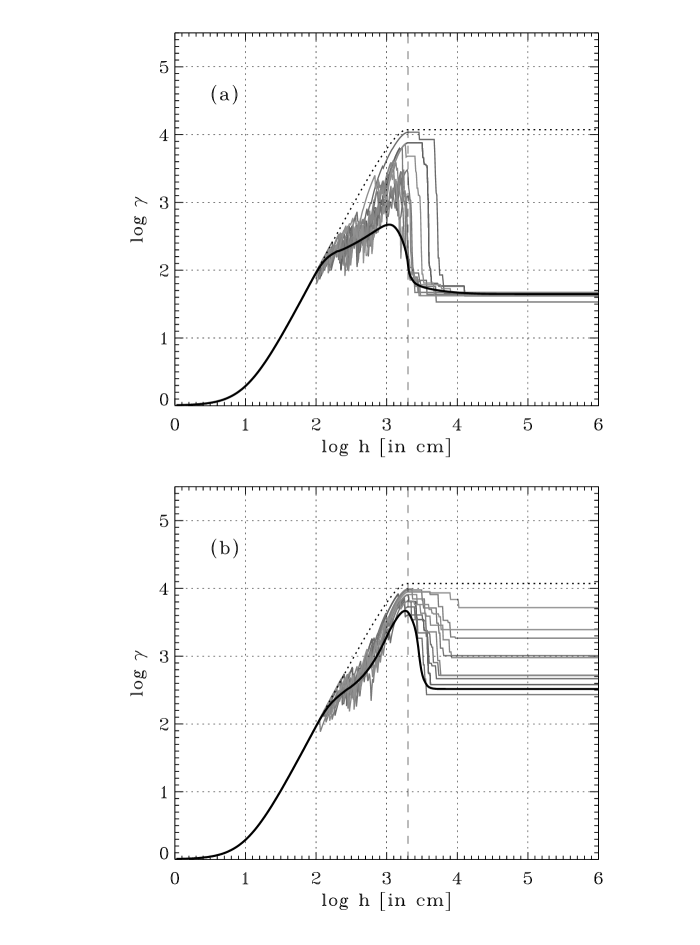
Figure 6: Electron Lorentz factor as a function of altitude for the HM98 electric field (Eq.2) with $h_{\rm acc}=2\times 10^{3}$ cm. Solution found with the integration method (thick solid line) is overplotted on ten Monte Carlo tracks. Thick dotted line is for the case with no radiative damping. The dashed vertical marks $h=h_{\rm acc}$. a case of $R_{\rm th}=10^{5}$ cm and $T_{6}=3.5$; b case of $R_{\rm th}=4\times 10^{3}$ cm and $T_{6}=3.0$; the other pulsar parameters are the same as in Fig. 1.

An effect similar to that shown in Fig. 1 appears, however, when the resonant ICS losses are no longer effective above $h=h_{\rm acc}$. Fig. 6b shows the case with $R_{\rm th}=4.0\times 10^{3}$ cm $=2\times h_{\rm acc}$ and $T_{6}=3.0$. Broad electron energy distribution (with average energy much exceeding a value from the integration method) emerges.

Similarly as in the weak electric field case, the position of the diffusion region in $T$-$B_{\rm pc}$ plane (for a fixed value of $R_{\rm th}$) is here determined with a condition analogous to Eq. (13) (but $E_{\parallel}$ of Eq.(2) requires a more accurate determination of $h_{\rm acc}$) along with a requirement for strong $B_{\rm pc}$ and low $T$.

For stronger electric fields ($E_{\parallel}>E_{\parallel}^{\rm eq}$), or for larger acceleration lengths the resonant ICS has negligible influence on final electron energies. In the first case acceleration greatly dominates the ICS damping; in the second case acceleration is stopped only over a negligible, initial part of accelerator height.

4 Conclusions

We have calculated the efficiency of energy losses for electrons accelerated over a hot polar cap of a neutron star. As cooling mechanisms we have considered the inverse Compton scattering and the curvature radiation, (though the latter has been negligible for the considered acceleration models).

The electron energy losses due to the ICS have been calculated with the Monte Carlo method and compared with the integration method (after Chang chang (1995); Sturner sturner (1995)) based on the prescription for the averaged ICS cooling (Dermer dermer (1990)). We confirm general predictions of the integration approach (eg. the limitation of electron Lorentz factors below $\sim 10^{2}$ for high temperatures), nevertheless, the “stopping acceleration effect” occurs at a slightly higher temperature than that one resulting from integrating the differential equation (12).

For the considered pulsar parameters ($B_{\rm pc}=15.8\times 10^{12}$ G, $R_{\rm th}=10^{5}$ cm) and the acceleration potential by Michel (michel (1974)), the Monte Carlo-based value is approximately equal to $T_{\scriptscriptstyle\rm MC}=4.5\times 10^{6}$ K (at this $T$ only a few percent of electrons reach $\gamma>10^{2}$ at $h=10^{6}$ cm) in comparison with $T_{\rm int}=3.3\times 10^{6}$ as given by the integration approach. Although the temperature difference is small, the final electron Lorentz factors as determined by the two methods may easily differ by a few orders of magnitude (Fig. 1, the case $T_{6}=3.5$) if the observed temperature matches this range. Moreover, it should be kept in mind that for most objects with hard X-ray emission identified putatively as originating from the hot polar cap, temperatures lie within the similar range $(2-4)\times 10^{6}$ K (Ögelman ogelman (1995)).

We find that for high-$B$ and low-$T$ pulsars the integration method gives a poor estimation of electron Lorentz factors if the energy loss rate due to the resonant ICS hardly exceeds the rate of acceleration. In the case of Michel’s model and for $R_{\rm th}>h_{\rm acc}$, this occurs if $T\sim 4(B_{12}P)^{-1/4}$ which may be the case for PSR B1509$-$58. In the cases when the ICS loss rate dominate firmly over the acceleration or is negligible the energy distribution of outgoing electrons is quasi-monoenergetic around the value which is well approximated with the continuous approach.

We find that preventing electrons from achieving large Lorentz factors occurs also for accelerating potential by Harding & Muslimov (hm (1998)) in its nonsaturated version with $h_{\rm acc}\ll r_{\rm pc}$. The discrepancy between the Monte Carlo and the integration method also occurs within the high-$B$ and low-$T$ regime and is especially pronounced for $R_{\rm th}\sim h_{\rm acc}$.

- (1) Arons J., 1996, A&AS, 120, 49
- (2) Arons J. & Scharlemann E.T., 1979, ApJ, 231, 854
- (3) Becker W. & Trümper J., 1997, A&A, 326, 682
- (4) Chang H.K., 1995, A&A, 301, 456
- (5) Daugherty J.K. & Harding A.K., 1986, ApJ, 309, 362
- (6) Daugherty J.K. & Harding A.K., 1989, ApJ, 336, 861
- (7) Dermer C.D., 1990, ApJ, 360, 197
- (8) Harding A.K. & Muslimov A.G., 1998, ApJ, 508, 328 (HM98)
- (9) Herold H., 1979, Phys. Rev. D, 19, 2868
- (10) Ho C. & Epstein R.I., 1989, ApJ, 343, 277
- (11) Kardashëv N.S., Mitrofanov I.G., Novikov I.D., 1984, Soviet Astron., 28, 651
- (12) Kuiper L., et al., 1999, A&A, 351, 119
- (13) Michel F.C., 1974, ApJ, 192, 713 (M74)
- (14) Muslimov A.G. & Tsygan A.I., 1992, MNRAS, 255, 61
- (15) Ögelman H.: 1995, X-Ray Observations of Cooling Neutron Stars. In: The Lives of the Neutron Stars, Alpar M.A., et al. (eds.), Kluwer, 101
- (16) Pavlov G.G., Shibanov Y.A., Ventura J., Zavlin V.E., 1994, A&A, 289, 837
- (17) Saito Y., Kawai N., Kamae T., Shibata S., 1998, In: Proc. of the International Conference on Neutron Stars and Pulsars, Shibazaki N., Kawai N., Shibata S., et al. (eds.), Universal Academy Press, Tokyo, 295
- (18) Sturner S.J., 1995, ApJ, 446, 292
- (19) Sturner S.J. & Dermer C.D., 1994, ApJ, 420, L79
- (20) Sturner S.J., Dermer C.D., Michel F.C., 1995, ApJ, 445, 736
- (21) Supper R. & Trümper J., 2000, A&A, 357, 301
- (22) Xia X.Y., Qiao G.J., Wu X.J., Hou Y.Q., 1985, A&A, 152, 93
- (23) Zhang B. & Harding A.K., 2000, ApJ, 532, 1150