One relation for self-gravitating bodies

Abstract

The relation between the gravitational potential energy, the central potential, and the mass is considered for various self-gravitating bodies.

I Introduction

For homogeneous triaxial ellipsoid with semiaxes $A,\,B,\,C\,$ and density $\rho$ the next relations are valid (Landau and Lifshits 1975).The gravitational potential at the inner point ($X,\,Y,\,Z\,$), $-A\leq X\leq A$, $-B\leq Y\leq B$, $-C\leq Z\leq C$, is

$$\begin{array}[]{l}U_{ell}(X,Y,Z)=\pi\,\rho\,G\,A\,B\,C\,\int_{0}^{\infty}\,\biggl{(}1-{X^{2}\over A^{2}+s}-{Y^{2}\over B^{2}+s}-{Z^{2}\over C^{2}+s}\biggr{)}{\,d\,s\over Q_{s}};\\ Q_{s}=\sqrt{(A^{2}+s)(B^{2}+s)(C^{2}+s)}.\end{array}$$ (1)

The potential energy of the homogeneous triaxial ellipsoid is:

$$W_{ell}={3\over 10}G\,M^{2}\int_{0}^{\infty}{d\,s\over Q_{s}}.$$ (2)

Here $M_{ell}=4/3\,\pi\,\rho\,A\,B\,C$ is the ellipsoid’s mass and $G$ stands for Newtonian constant of gravitation. Note that gravitational energy of self-gravitating body is of negative sign but we loosely write all $W$s with positive sign. In general case $A\neq B\neq C$ the integrals in (1) and (2) are expressed only in terms of the incomplete elliptic integrals and this precludes any detailed analysis.  However, if we consider only potential at the center of ellipsoid, $U_{ell}(0,0,0)$, then we get the remarkable relation:

$$WUM={W_{ell}\over U_{ell}(0,0,0)\,M_{ell}}={2\over 5},$$ (3)

valid for any values of semi-axes. We shortly refer to this relation (3) as $WUM$-ratio.
Recently Seidov and Skvirsky (2000a) presented the gravitational potential and the potential energy for the homogeneous rectangular parallelepiped (hereafter RP) which allows to analyse this $WUM$-ratio for the new class of the homogeneous self-gravitating bodies.
In this paper, we show in sections II and III that the value of $WUM$ for RPs has minimal value $.395437$ (see Eq. (10)) for the cube (all three dimensions of RP equal to each other), tends to 1/2 for one dimension of RP far larger larger than two others (long thin ”stick” with square cross-section), and tends to ${1\over 2}-{\sqrt{2}-1\over 6\,\ln(\sqrt{2}+1)}=.421673$ as one dimension is far less than two others (thin square ”plate”), see Fig. 1.
Also, in section IV we discuss the $WUM$-ratio for homogeneous gravitating bodies studied recently by Kondrat’ev and Antonov (1993). We show that values of $WUM$-ratio for the homogeneous summetrical lenses are in the interval from $128/105\,\pi$, for infinitesimally thin symmetrical lens, to $17/20$, for two homogeneous equal spheres just touching each other.
In section VI we analyse $WUM$-ratio for spherical polytropic stars, and show that $WUM$-ratio varies from $2/5$ to $3/32\,\pi$ for polytropic index $n$ varying from $0$ to $5$.
In the section VII we discuss the interesting class of two-phase spheres and show that unlike the polytropes, in this case the $WUM$-ratio’s interval is larger: it is possible to get very small values of $WUM$ if the ratio of two densities $q=\rho_{2}/\rho_{1}$ is large enough and if the relative value of core’s radius is not too small.
At last, in the sections VIII and IX we consider another two simple classes of non-homogeneous bodies both allowing analytical treatment.

II Potential at the center of RP

Using results by Seidov and Skvirsky (2000a) we write down the gravitational potential at the center of the homogeneous RP with density $\rho$ and with edge lengths $2a,\,2b,\,2c$:

$$\begin{array}[]{l}U_{RP}(0,0,0)=4\,G\,\rho\,[a\,b\ln{d+c\over d-c}+b\,c\ln{d+a\over d-a}+cd\ln{d+b\over d-b}-\\ \\ a^{2}\arctan{b\,c\over a\,d}-b^{2}\arctan{a\,c\over b\,d}-c^{2}\arctan{a\,b\over c\,d}].\end{array}$$ (4)

Here $d=(a^{2}+b^{2}+c^{2})^{1/2}$ is the main diagonal of RP.
Three particular cases are of the larger interest:
a)cube corresponding to case $c=b=a$,

$$U_{cube}(0,0,0)=G\,\rho\,a^{2}\biggl{[}24\ln{1+\sqrt{3}\over\sqrt{2}}-2\pi\biggr{]}=9.52017\,G\,\rho\,a^{2};$$ (5)

b)long thin stick with square cross-section corresponding to case $a>>b=c$:

$$U_{stick}(0,0,0)=G\,\rho\,b^{2}(-8\,\ln{b\over a}+12-2\,\pi+4\,\ln 2);$$ (6)

c)thin square plate corresponding to the case $a<<b=c$:

$$\,U_{plate}(0,0,0)=G\,\rho\,[16\,a\,b\,\ln(\sqrt{2}+1)-2\,\pi\,a^{2}].$$ (7)

III Potential energy of RP

According to Seidov and Skvirsky (2000a) the gravitational potential energy of the homogeneous rectangular parallelepiped is equal to:

$$\begin{array}[]{l}WRP=G\,\rho^{2}[f(a,b,c)+f(b,c,a)+f(c,a,b)];f(a,b,c)=c_{5}a^{5}+c_{4}a^{4}+c_{3}a^{3}+c_{2}a^{2};\\ \\ c_{5}={32\over 15};\,\,c_{4}={32\over 15}(d-d1-d3)-{16\,b\over 3}\ln{(d1-b)(d+b)\over a\,d3}-{16\,c\over 3}\ln{(d3-c)(d+c)\over a\,d1};\\ \\ c_{3}=-{64\,b\,c\over 3}\arctan{b\,c\over a\,d};\quad d=\sqrt{a^{2}+b^{2}+c2};\,d1=\sqrt{a^{2}+b^{2}};\,d3=\sqrt{a^{2}+c^{2}};\\ \\ c_{2}={32\,b^{2}\over 5}(d1-d)+{32\,c^{2}\over 5}(d3-d)-16\,b\,{c^{2}}\,\ln{d-b\over d+b}-16\,{b^{2}}\,c\,\ln{d-c\over d+c}.\end{array}$$ (8)

A Potential energy and $WUM$-ratio of cube

From (8), taking $c=b=a$, we get the potential energy of homogeneous cube with edge length $2a$:

$$\begin{array}[]{l}W_{cube}=32G\rho^{2}a^{5}\{{2\sqrt{3}-\sqrt{2}-1\over 5}+{\pi\over 3}+\ln[(\sqrt{2}-1)(2-\sqrt{3})]\}=30.117\,G\rho^{2}a^{5}.\end{array}$$ (9)

From (5) and (9) we get $WUM$-ratio for homogeneous cube:

$$WUM_{cube}=2{{2\sqrt{3}-\sqrt{2}-1\over 5}+{\pi\over 3}+\ln[(\sqrt{2}-1)(2-\sqrt{3})]\over 24\ln{1+\sqrt{3}\over\sqrt{2}}-2\pi}=.395437.$$ (10)

B Potential energy and $WUM$-ratio of thin long stick

We take $a>>b=c$ that corresponds to the case of the thin long stick with the square cross-section. Leading term in expansion of WRP (8) gives the potential energy of the thin long stick:

$$W_{stick}={32\over 3}G\rho^{2}a\,b^{4}\ln{a\over b}.$$ (11)

From this and (6) we get for stick:

$$WUM={W_{stick}\over 8\,a\,b^{2}U_{stick}(0,0,0)}={1\over 2}.$$ (12)

C Potential energy and $WUM$-ratio of thin square plate

Taking one of RP’s dimension infinitesimally small, $a\rightarrow 0$, we get, from Eq.(8), the potential energy of the thin rectangular plate. If we additionally take $b=c$, then we get the potential energy of the thin square plate ($a<<b$):

$$W_{pl}=64\,G\,\rho^{2}b^{3}\,a^{2}\,\left(\ln(\sqrt{2}+1)-{\sqrt{2}-1\over 3}\right)=47.5714\,G\,\rho^{2}b^{3}a^{2}.$$ (13)

From (7) and (13) we have another limit for value of $WUM$:

$${WS\over 8\,a\,b^{2}U_{pl}(0,0,0)}={1\over 2}-{\sqrt{2}-1\over 6\,\ln(\sqrt{2}+1)}=.421673.$$ (14)

FIG. 1.: WUM for RP with square cross section $2\,b\,$x$\,2\,b$ and length $2\,a$. Abscissas are values of $b/a$ and ordinates are values of relation $WUM=W/U(0)\,M$ that is ratio of gravitational potential energy of RP to product of gravitational potential at the center of RP by mass of homogeneous RP. $WUM$ has minimum for cube ($b/a=1$), tends to 1/2 at $b/a\rightarrow 0$ (thin long stick) and to ${1\over 2}-{\sqrt{2}-1\over 6\,\ln(\sqrt{2}+1)}=.421673$ (dash line ) at $b/a\rightarrow\infty$ (thin square plate). For homogeneous ellipsoid, $WUM=2/5$, solid line.

D Relation between potential energy, gravitational potential and mass of RP

General behavior of relation between the potential energy, the gravitational potential at the center, and mass of the homogeneous RP with two equal edge-lengths is shown in the Fig. 1, which is a result of numerical calculation by the formulas (4) and (8). For homogeneous ellipsoid $WUM=2/5$, see (3), solid line in Fig. 1.

IV Homogeneous symmetric lenses

Recently Kondrat’ev and Antonov (1993) (hereafter KA) have obtained the analytical formulas for the gravitational potential and the gravitational energy of some axial-symmetric figures, namely homogeneous lenses with spherical surfaces of different radii. In forthcoming paper (Seidov and Skvirsky 2000b) we present some new solutions for homogeneous bodies of revolution.
Here we present the review of $WUM$ for most suitable kind of those bodies, discussed by KA, namely the homogeneous symmetrical lenses. A segment of sphere, or a planoconvex lens, is obtained by cutting a sphere with a plane. If $R$ is a radius of a sphere, $h$ is height of segment, and $2\,a$ is a radius of segment’s base, then $a=\sqrt{2\,h\,R-h^{2}}$. A symmetric homogeneous lens (SL) is obtained by placing together the bases of two identical segments of sphere.
According to KA we have for the gravitational potential at the center of such SL:

$$U_{SL}(0)={4\,\pi\,G\,\rho\over 3}\left(h\,R+R^{2}-{h^{2}\over 2}+{R^{3}-a^{3}\over h-R}\right).$$ (15)

The gravitational energy of SL is:

$$\begin{array}[]{l}W_{SL}={4\,\pi\,G\,{\rho}^{2}\over 9}\biggl{[}10\,R^{4}\,a-{16\over 3}\,R^{2}\,a^{3}-{8\over 3}\,a^{5}+\pi\,{h^{4}}\,({2\over 5}\,h-2\,R-{R^{2}\over R-h})+2\,{R^{4}}\,\biggl{(}{R^{2}\over R-h}-6\,(R-h)\biggl{)}\,\arctan{a\over R-h})\biggr{]}.\end{array}$$ (16)

And the total mass of the homogeneous SL is:

$$M_{SL}={2\,\pi\,\rho\,h^{2}\over 3}\,(3\,R-h).$$ (17)

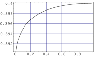
FIG. 2.: WUM for SL. Abscissas are values of $h/R$, ratio of height of half-lens to radius of sphere and ordinates are values of relation $WUM=W/U(0)\,M$. At $h/R\rightarrow 0$ (thin spherical lense), $WUM\rightarrow{128\over 105\,\pi}=.388035$. At $h/R\rightarrow 1$, (full sphere) $WUM\rightarrow 2/5$.

We may consider $WUM$-ratio for such bodies as $W_{SL}/U_{SL}\,M_{SL}$. Defined so, $WUM$ for the homogeneous symmetric lenses has general dependence on parameter $h/R$, according the formulas (15), (16) and (17), as shown in the Fig. 2. Note that in the limit $h/R\rightarrow 0$ we have infinitesimally thin symmetrical lens with radius of curvature tending to infinity, and we have:

$$Limit[WUM_{SL}]_{h/R\,->0}={128\over 105\,\pi}=.388035.$$ (18)

Interestingly, this infinitesimally thin round lens does not coincide at all with the case of the infinitesimally thin quadratic plane which has the much more larger value of $WUM=.421673$ (see Eq.(14)). In another limit $h/R\rightarrow 1$ we have a full homogeneous sphere, and evidently:

$$Limit[WUM_{SL}]_{h/R->1}=2/5.$$ (19)

There is still another $analytical$ case at $h\rightarrow 2\,R\,$ when we have two homogeneous spheres touching each other so that distance between centers of spheres is $d=2\,R;$ then ”potential at the center of SL” is $U_{SL}(0)=2\,{G\,M\over R}$; potential energy is sum of two terms: proper potential energy of each spheres $2\,{3\over 5}\,{G\,M^{2}\over R}$, and $interaction$ energy, ${G\,M^{2}\over d}$ or ${G\,M^{2}\over 2\,R}$; we have:

$$WUM_{SL}|_{h=2\,R}=({1\over 2}+{6\over 5})/2={17\over 20}.$$

V Heterogeneous spherical bodies

Now we consider the problem of $WUM$-ratio from another point of view. Abovementioned homogeneous gravitating bodies (ellipsoids, right parallelepipeds, and symmetrical spherical lenses) differ from each other only by their forms and so $WUM$-ratio may be referred to as form-factor. As it is evident, $WUM$-ratio should be also function of density distribution over the body. If we confine ourselves by spherically-symmetric distribution of density $\rho(r)$, then we have general expressions for the gravitational potential at radius $r$:

$$U(r)={G\,m(r)\over r}+\int_{r}^{R}\,4\,\pi\,G\,\rho(r)\,r\,dr;$$ (20)

central potential:

$$U(0)=\int_{0}^{R}\,4\,\pi\,G\,\rho(r)\,r\,dr;$$ (21)

potential energy:

$$W={1\over 2}\,\int_{0}^{M}\,U(r)\,dm(r);$$ (22)

and mass:

$$dm=4\,\pi\,\rho(r)\,r^{2}\,dr;\quad M=\int_{0}^{R}\,4\,\pi\,\rho(r)\,r^{2}dr.$$ (23)

From these expressions we write down $WUM$ for spherical-summetrical heterogeneous bodies as:

$$WUM={W\over U(0)\,M}={1\over 2}{\overline{U}\over U(0)};\quad\overline{U}={1\over M}\int_{0}^{M}\,U(m)\,dm.$$ (24)

As a result, $WUM$-ratio of spherically-symmetric bodies is reduced to the ratio of the mean value of monotonic function, $U(m)$, to its particular value, $U(0)$, (ratio being additionally divided by 2). The boundary values of this ratio can be found pure mathematically for any given class of functions $\rho\,(r)$. We will not deal with this abstract (though interesting) problem; instead, in the next sections we consider two cases of more or less realistic bodies, namely polytropes and two-phase spheres.

VI Polytropes

One case of heterogeneous bodies which apparently should be considered first is the case of classical polytropic stars. Using formulas from Chandrasekar’s (1957) classical text we have (some of these formulas are valid not only for polytropic stars but we do not stop on these details) the next relations.
a)central potential is expressed via other parameters of star as follows (Chan 100/85= Chandrasekhar (1957), p.100, Eq. (85)):

$$U_{p}(0)=(n+1){P_{c}\over\rho_{c}}+{G\,M\over R}.$$ (25)

Here $n$ is the polytropic index, $P_{c}$ and $\rho_{c}$ are central values of pressure and density, $M$ and $R$ are the mass and radius of the star.
The next formulas include the parameters of the Lane-Emden function (LEF) at the first zero point:

$$\begin{array}[]{l}\xi=\xi_{1},\quad\theta(\xi=\xi_{1})\equiv\theta_{1}=0;\quad\biggr{[}{d\,\theta\,(\xi)\over d\,\xi}\biggr{]}_{\,\xi=\xi_{1}}\equiv\,{\theta_{1}}^{\prime}\,<\,0;\quad\mu_{1}=-\,\xi_{1}^{2}\,{\theta_{1}}^{\prime}.\end{array}$$ (26)

Central pressure is (Chan 99/80,81):

$$P_{c}={1\over 4\,\pi\,(n+1)({\theta_{1}}^{\prime})^{2}}{\,G\,M^{2}\over R^{4}}.$$ (27)

Central density $\rho_{c}$ is related with the mean density $\overline{\rho}$ of the star as follows (Chan 78/99):

$$\rho_{c}={1\over 3}\quad{\xi\over-{\theta_{1}}^{\prime}}\quad\overline{\rho}.$$ (28)

Combining these formulas we get the final expression for the central potential of polytropic star:

$$U_{p}(0)=\biggl{(}1+\quad{1\over-\,\xi_{1}\,{\theta_{1}}^{\prime}}\biggr{)}{G\,M\over R}.$$ (29)

b)potential energy
We have for polyropic star the famous formula (Chan 101/90):

$$W_{p}={3\over 5-n}{G\,M^{2}\over R}.$$ (30)

c)WUM-ratio:

$$WUM_{p}={3\over 5-n}\quad{1\over 1+\,{\xi_{1}\over\mu_{1}}}.$$ (31)

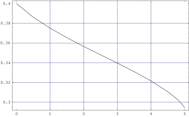
FIG. 3.: $WUM$ for polytropes. Abscissas are values of polytropic index $n$ and ordinates are values of the $WUM$-ratio.

A $WUM$-ratio for polytropes

Using values of parameters of polytropic stars given in (Chan, Table 4, p. 96) we calculated the values of $WUM$-ratio for values of polytropic index $n$ from $0$ to $4.9$, see Fig. 3. However the limit $n\rightarrow 5$ and in general region of values of $n$ close to 5 should be considered separately. First we note that at $n\rightarrow 5$, $\quad\xi_{1}\rightarrow\infty$ and there is indeterminacy of $\infty\over\infty$ kind in formula for $WUM_{p}$ Eq. (31). To solve this problem we use results of Seidov and Kuzakhmedov (1979) who obtained, in particular, the dependence of $\xi_{1}$ for $n$ close to 5:

$$(0\,<\,(5-n)/5\,<<\,1),\quad\xi_{1}\,=\,{32\,\sqrt{3}\over\pi}\,\,{1\over 5-n}.$$ (32)

Also it was shown by Seidov and Kuzakhmedov (1979) that for values of $n$ close to 5, the parameter $\mu_{1}$ is an increasing function of $n$:

$$\mu_{1}=\sqrt{3}\,(1+{1\over 12}\,\,{1\over 5-n}),$$ (33)

that means that $\mu_{1}$ has minimum at $n$ about 4.82. This may or may not lead to minimum of $WUM_{p}$ as function of $n$. At point $n=5$ using LEF of index 5:

$$n=5,\quad\theta(\xi)=(1+{1\over 3}\,\xi^{2})^{-1/2},$$ (34)

we get

$$n=5,\quad WUM_{p}\,=\,{3\over 32}\,\pi=.294524.$$ (35)

Additionally we have two other analytical results for $WUM$ of polytropes : at $n=0$, $\,WUM=2/5$ and at $n=1$, $\,WUM=3/8$. We recalculated the parameters of polytropes in the interval of $n$ from 4 to 5 and found no minimum for $WUM$, see Fig. 3. However we note that our boundary values differ from ones calculated by Jabbar (1993) in the sense that ours are less than his. As one example, at $n=4.7$ Jabbar gives $\xi_{1}=54.810686$ as zero of LEF, while our calculations using Mathematica’s command NDSolve give $\theta(54.810686)=-4.5910^{-7}$ and our value of $\xi_{1}$ is in interval between $\xi=54.8098$ (at this point $\theta=4.98*10^{-}8$) and $\xi=54.8099$ (at this point $\theta<0$). In general our values of $\xi_{1}$ are less than Jabbar’s.

VII Two-phase sphere

If $\rho_{1}$ and $\rho_{2}=q\,\rho_{1}$ are densities in envelope and core of sphere, and $R$ and $r=x\,R$ are total radius of sphere and radius of core, then we have next relations:
a)gravitational potential at the center:

$$U_{2ph}(0)=2\,\pi\,G\,\rho_{1}\,R^{2}\,[1+(q-1)\,x^{2}];$$ (36)

b)potential energy:

$$W_{2ph}={16\,{\pi}^{2}\,G\over 15}{\rho_{1}}^{2}\,R^{5}\,[1+{5\over 2}(q-1)\,x^{3}+(q-1)(q-{3\over 2})\,x^{5}];$$ (37)

c)total mass:

$$M_{2ph}={4\,\pi\over 3}\,\rho_{1}\,R^{3}\,[1+(q-1)\,x^{3}];$$ (38)

d)$WUM\,-\,ratio$:

$$\begin{array}[]{l}WUM_{2ph}={2\over 5}{1+{5\over 2}(q-1)\,x^{3}+(q-1)(q-{3\over 2})\,x^{5}\over[1+(q-1)\,x^{2}]\,[1+(q-1)\,x^{3}]}.\end{array}$$ (39)

FIG. 4.: $WUM$ for two-phase spheres. Abscissas are values of relative radius of core, and ordinates are values of the $WUM$-ratio. Dash line shows the locus of minimuma of $WUM$.

In Fig.4 we present dependence of $WUM$-ratio, for two-phase spheres with various values of $q$, as function of relative radius of core $x=r/R$. Curves from uppper one to lower one correspond to values of $q=3,\,5,\,10,\,$ and $20$, respectively. Both values of minimuma of $WUM$ and their ”places”, corresponding values of $x$, are decreasing functions of $q$. For values of $x$ corresponding to minimuma of $WUM$ the next simple equation is valid:

$$6\,q^{2}\,x^{5}+5\,q\,(1-x)\,x^{3}\,(1+2\,x)-(1-x)^{3}\,(4+7\,x+4\,x^{2})=0.$$ (40)

or

$$q=\frac{(1-x)\,\left(\sqrt{96/x+97+28\,x+4\,x^{2}}-5-10\,\sqrt{x}\right)}{12\,x^{2}}.$$ (41)

We used these formulas to calculate the dash line in Fig. 4.

VIII Stepenars

Here we briefly consider the case of simple spherically-symmetric density distribution law allowing analytical expression for WUM. We take:

$$\rho(r)=\rho_{c}\,(1-r/R)^{\nu},$$ (42)

where $\rho_{c}$ is central density and $\nu$ is a free parameter. By historical reasons we refer to the gravitating bodies with density distribution (42) as ”stepenars”, (Seidov, Kasumov, and Guseinov 1971).
We have:
mass:

$$M={8\,\pi\,\rho_{c}R^{3}\over(1+\nu)(2+\nu)(3+\nu)};$$ (43)

mean-to-central density ratio:

$${\overline{\rho}\over\rho_{c}}={6\over(1+\nu)(2+\nu)(3+\nu)};$$ (44)

central potential:

$$U(0)={4\,\pi\,G\,\rho_{c}R^{2}\over(1+\nu)(2+\nu)};$$ (45)

potential energy:

$$W={8\,\pi^{2}\,G\,\rho_{c}R^{2}\,(8+5\,\nu)\over(1+\nu)^{2}(2\,+\nu)^{2}(3+2\,\nu)(5+2\,\nu)};$$ (46)

WUM-ratio:

$$WUM_{\nu}={(3+\nu)(8+5\,\nu)\over 4\,(3+2\,\nu)(5+2\,\nu)}.$$ (47)

FIG. 5.: $WUM$ for stepenars. Abscissas are values of parameter $\nu$ in density distribution law $\rho(r)=\rho_{c}\,(1-r/R)^{\nu}$, and ordinates are values of $WUM$-ratio. Broken line shows asimptotic value of $WUM\rightarrow 5/16$ at $\nu\rightarrow\infty$.

In Fig. 5 the dependence of $WUM$-ratio for stepenars as function of parameter $\nu$ is shown. In spite of large variation of matter concentration from $\rho=const$ at $\nu=0$, to $\overline{\rho}/\rho_{c}\rightarrow 0$ at $\nu\rightarrow\infty$, $WUM$-ratio again as in polytrope’s case lies in rather limited interval from $2/5$ to $5/16$.

IX Alphars

Here we consider another example of ”exotic” but simple density distribution, Seidov and Seidova (1971):

$$\rho(r)=\rho_{c}\,(r/R)^{\alpha},\quad 0\leq\alpha\leq 2.$$ (48)

We have:

$$WUM_{\alpha}={2-\alpha\over 5-2\,\alpha}.$$ (49)

X Discussion

There is a rather classic problem of looking for general theorems of stellar structure, see e.g. chapter 3 in the classic text Chandrasekhar (1957). The problem considered in this paper may be also referred to as that dealing with general structure of celestial self-gravitating bodies.
We start from interesting observation on one constant ratio, namely, (potential energy W)/((central potential U ) x (total mass M)), in homogeneous ellipsoids and then try to look for behavior of this ratio for another homogeneous bodies: rectangular parallelelepipeds and symmetrical lenses. We found that in both cases $WUM$-ratios are confined in rather narrow interval. Suprisingly, dependence of $WUM$ for homogeneous rectangular parallelepipeds (RP) on edge lengths ratio is non-monotonic: it has minimal value $.395437$ for cube while any deviation from cube form to prolate RP (one dimension being smaller than two others) or elongated RP (one dimension being larger that two others) leads to the increase of value of $WUM$. In this respect the behavior of homogeneous rectangular parallelepipeds is quite unlike the behavior of homogeneous ellipsoids and there is still some mystery even to authors.
As to the homogeneous symmetrical lenses (SL) by Kondrat’ev and Antonov (1993), here the dependence of $WUM$ on parameters of SL is monotonic, however in this case there is also some suprise in the sense that in the limiting case of thin symmetrical $spherical$ lens the $WUM$-ratio’s value, ($128/105\,\pi$), differs radically from the case of the infinitesimally thin $quadratic$ plate with $WUM=1/2$.
Then we look for the non-homogeneous however spherically symmetric bodies and found that for the polytropes with polytropic index $n$ in the interval $0-5$, $WUM$-ratio again lies in narrow interval from $2/5$ to $3/32\,\pi$. However for two-phase sphere with large ratio of densities $q=\rho_{2}/\rho_{1}$ it is possible to get very small values of WUM. The physical reason of it is that if we put in the center of any spherical symmetric star a (very) small but dense spherical body then central potential may be very large while total potential energy of star, being integral value, increases not so drastically. The effect of the strong variation of density in the center of star, the ”first-order phase-transition”, is known since pioneer works of W.H. Ramsey (1950).
In last two paragraphs of paper we consider pure mathematical toy models in further attempts to understand the behavior of the $WUM$-ratio. We conclude this discussion with notice that central-to-surface potential ratio $U(0)/U(R)$ (among other ”global” characteristics of the celestial self-gravitating configurations) is also worth studying. For polytropes, $U(0)/U(R)=1+\xi_{1}/\mu_{1}$, see section VI.

REFERENCES

• [1] Chandrasekhar, S. 1975. An introduction to stellar structure study. Dover, N.Y.
• [2] Jabbar, J.R.. 1994, Astrophys. Sp. Sci. 100, 447.
• [3] Kondrat’ev, B.P. 1993, Astron. Rep. 37 (2), 295;
Kondrat’ev, B.P., Antonov, V.A., Astron. Rep. 37 (3), 300.
• [4] Landau, L.D., Lifshits, E.M. 1975. The classical theory of fields. Pergamon Press, Oxford.
• [5] Ramsey, W.H. 1950. Mon. Not. Roy. Astron. Soc. 110, 325.
• [6] Seidov, Z.F., Kasumov F.K., Guseinov, O.Kh. 1971, Cirkuliar Shemakh. Astrophys. Observ. no. 3, 4-5.
• [7] Seidov, Z.F., Kuzakhmedov, R.Kh. 1979, Sov. Astron - AJ 22,  711.
• [8] Seidov, Z.F., P.I. Seidova, P.I. 1971, Cirkuliar Shemakh. Astrophys. Observ. no. 16, 10-13.
• [9] Seidov, Z.F., P.I. Skvirsky, P.I. 2000a, astro-ph/0002496.
• [10] Seidov, Z.F., P.I. Skvirsky, P.I. 2000b, in preparation.