Abstract

Using a simple combinatorial algorithm for generating finite and discrete events as our numerical cosmology, we predict that the baryon/photon ratio at the time of nucleogenesis is $\eta=1/256^{4}$, $\Omega_{DM}/\Omega_{B}=12.7$ and (for a cosmological constant of $\Omega_{\Lambda}=0.6\pm 0.1$ predicted on general grounds by E.D.Jones) that $0.325>\Omega_{M}>0.183$. The limits are set not by our theory but by the empirical bounds on the renormalized Hubble constant of $0.6<h_{0}<0.8$. If we impose the additional empirical bound of $t_{0}<14\ Gyr$, the predicted upper bound on $\Omega_{M}$ falls to $0.26$. The predictions of $\Omega_{M}$ and $\Omega_{\Lambda}$were in excellent agreement with Glanz’ analysis in 1998, and are still in excellent agreement with Lineweaver’s recent analysis despite the reduction of observational uncertainty by close to an order of magnitude.

The theory on which I base my predictions is unconventional. Hence it is easier for me to show you first the consequences of the predictions in comparison with observation, in order to establish a presumption that the theory might be interesting, and then show you how these predictions came about.

The predictions are that (a) the ratio of baryons to photons was $\eta=1/256^{4}=2.328...\times 10^{-10}=10^{-10}\eta_{10}$ at the time of nucleogenesis, (b) $\Omega_{DM}/\Omega_{B}=127/10=12.7$ and (c) $\Omega_{\Lambda}=0.6$. Comparison of prediction (a) with observation is straightforward, as is illustrated in Figure 1.

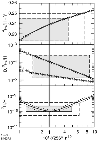
Figure 1: Comparison of the bit-string physics prediction that $\eta=256^{-4}$ with accepted limits on the cosmic abundances as given by Olive and Schramm in [19], p. 119.

Comparison with observation of prediction (b) that the ratio of dark to baryonic matter is not straightforward, as was clear at DM98; I suspect that is matter will remain unresolved at this conference (DM2000). However, according to the standard cosmological model, the baryon-photon ratio remains fixed after nucleogenesis. In the theory I am relying on, the same is true of the of the dark matter to baryon ratio. Consequently, if we know the Hubble constant, and assume that only dark and baryonic matter contribute, the normalized matter parameter $\Omega_{M}$ can also be predicted, as we now demonstrate.

We know from the currently observed photon density (calculated from the observed $2.728\ ^{o}K$ cosmic background radiation) that the normalized baryon density is given by [18]

$$\Omega_{B}=3.67\times 10^{-3}\eta_{10}h_{0}^{-2}$$ (1)

and hence, from our prediction and assumptions about dark matter, that the total mass density will be 13.7 times as large. Therefore we have that

$$\Omega_{M}=0.11706h_{0}^{-2}\ .$$ (2)

Hence, for $0.8\geq h_{0}\geq 0.6$ [7], $\Omega_{M}$ runs from $0.18291$ to $0.32517$. This clearly puts no restriction on $\Omega_{\Lambda}$.

Our second constraint comes from integrating the scaled Friedman-Robertson-Walker (FRW) equations from a time after the expansion becomes matter dominated with no pressure to the present. Here we assume that this initial time is close enough to zero on the time scale of the integration so that the lower limit of integration can be approximated by zero [21]. Then the age of the universe as a function of the current values of $\Omega_{M}$ and $\Omega_{\Lambda}$ is given by

$$t_{0} = 9.77813h_{0}^{-1}f(\Omega_{M},\Omega_{\Lambda})\ Gyr$$ (3)

$$= 9.77813h_{0}^{-1}f(0.11706h_{0}^{-2},\Omega_{\Lambda})\ Gyr$$

where

$$f(\Omega_{M},\Omega_{\Lambda})=\int_{0}^{1}dx\sqrt{{x\over\Omega_{M}+(1-\Omega_{M}-\Omega_{\Lambda})x+\Omega_{\Lambda}x^{3}}}\ .$$ (4)

For the two limiting values of $h_{0}$, we see that

$$h_{0} = 0.8,\ \ t_{0}=12.223f(0.18291,\Omega_{\Lambda})\ \ Gyr$$

$$h_{0} = 0.6,\ \ t_{0}=16.297f(0.32517,\Omega_{\Lambda})\ \ Gyr\ .$$ (5)

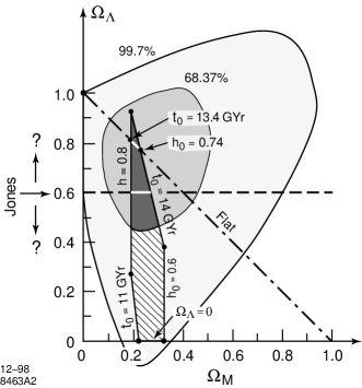
Figure 2: Limits on $(\Omega_{M},\Omega_{\Lambda})$ set by combining the Supernovae Type Ia data from Perlmutter, et al. with the Cosmic Ray Background Experiment (COBE) satellite data as quoted by Glanz [4] (dotted curves at the 68.37% and 99.7% confidence levels) compared with the predictions of bit-string physics that $\eta_{10}=10^{10}/256^{4}$ (cf. Fig. 1) and $\Omega_{\rm Dark}/\Omega_{B}=12.7$. We accept the constraints on the scaled Hubble constant $h_{0}=0.7\pm 0.1$ [6] and on the age of the universe $t_{0}=12.5\pm 1.5\ Gyr$ (solid lines). We include the predicted constraint $\Omega_{\Lambda}>0)$. The Jones estimate of $\Omega_{\Lambda}=0.6$ is indicated, but the uncertainty was not available in 1998.

The results are plotted in Figure 2. We emphasize that these predictions were made and published over a decade ago when the observational data were vague and the theoretical climate of opinion was very different from what it is now. The figure just given was presented at ANPA20 (Sept. 3-8, 1998, Cambridge, England) and given wider circulation in[14]. The calculation (c) that $\Omega_{\Lambda}=0.6$ was made by Jones before there was any observational evidence for a cosmological constant, let alone a positive one[3]. The precision of the relevant observational limits has improved

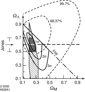
Figure 3: Limits on $(\Omega_{M},\Omega_{\Lambda})$ set by combining the Supernovae Type Ia data from Perlmutter, et al. with the Cosmic Ray Background Experiment (COBE) satellite data as quoted by Glanz [4] (dotted curves at the 68.37% and 99.7% confidence levels) and more recent much improved limits according to Lineweaver[8] (solid curves at $1\sigma,2\sigma,3\sigma$) compared with the predictions of bit-string physics that $\eta_{10}=10^{10}/256^{4}$ (cf. Fig. 1) and $\Omega_{DM}/\Omega_{B}=12.7$. We accept the constraints on the scaled Hubble constant $h_{0}=0.7\pm 0.1$ [6] and on the age of the universe $t_{0}=12.5\pm 1.5\ Gyr$ (solid lines). The Jones estimate of $\Omega_{\Lambda}=0.6\pm 0.1$ is included.

considerably since DM98. A recent analysis of this new data suitable for our purposes has been made by Lineweaver[8]. His one, two and three $\sigma$ contours are plotted in comparison with the previous observational limits and our (unchanged) earlier predictions in Figure 3. Note how dramatically the regions of uncertainty have shrunken in two years. It is gratifying that our prior predictions are still close to the center of the allowed region, indicating that it will take a lot more work to show that they are wrong!

The theory I am using has a long history[12], starting with the discovery of the combinatorial hierarchy in 1961 [20] and the first publication of the work on this idea by Amson, Bastin, Kilmister and Parker-Rhodes in 1966[1]. The theory is unusual in that it starts from minimal assumptions about what is needed for a physical theory and tries to let the structure of the theory grow out of them. My own preferred choice of basic assumptions are that a physicist must (a) be able to tell something from nothing, (b) be able to tell whether things are the same or different, and (c) must assume a basic arbitrariness in the universe which underlies the stochastic effects exhibited by quantum events. I further assume that we should use the simplest possible mathematical structures to model and develop these concepts. (a) is simply modeled by bit multiplication; (b) is simply modeled by bit addition (addition modulo 2, XOR, symmetric difference,…) or, as it is referred to in the ANPA program, discrimination.

The third requirement, together with the usual scientific assumption that we can keep historical records and examine them at later times, is accomplished by constructing a computer model called program universe[9, 16, 13] which yields a growing universe of ordered strings of the integers “0” and “1”. Here we remind the reader of how we use discrimination (“$\oplus$”) between ordered strings of zeros and ones (bit-strings) defined by

$$({\bf a}(W)\oplus{\bf b}(W))_{w}=(a_{w}-b_{w})^{2};\ \ a_{w},b_{w}\in 0,1;\ \ w\in 1,2,....,W$$ (6)

to generate a growing universe of bit-strings which at each step contains $P(S)$ strings of length $S$. The algorithm is very simple, as can be seen from the flow diagram in Fig. 4. We start with a rectangular block of rows and columns containing only the bits “0” and “1”. We then pick two rows arbitrarily and if their discriminant is non-null, adjoin it to the table as a new row. If it is null, we simply adjoin an arbitrary column (Bernoulli sequence) to the table and recurse to picking two arbitrary rows. That this model contains arbitrary elements and (if interpretable in terms of known aspects of the practice of physics) an historical record (ordered by the number of TICK’s, or equivalently by the row length) should be clear from the outset. The forging of rules that will indeed connect the model to the actual practice of physics is the primary problem that has engaged me ever since the model was created.

Figure 4: Flow diagram for constructing a bit-string universe growing by one row or one column at a time (see text).

Program universe provides a separation into a conserved set of “labels”, and a growing set of “contents” which can be thought of as the space-time “addresses” to which these labels refer. To see this, think of all the left-hand, finite length $S$ portions of the strings which exist when the program TICKs and the string-length goes from $S$ to $S+1$. Call these labels of length $L=S$, and the number of them at the critical tick $N_{0}(L)$. Further PICKs and TICKs can only add to this set of labels those which can be produced from it by pairwise discrimination, with no impact from the (growing in length and number) set of content labels with length $S_{C}=S-L>0$. If $N_{I}\leq N_{0}(S_{L})$ of these labels are discriminately independent, then the maximum number of distinct labels they can generate, no matter how long program universe runs, will be $2^{N_{I}}-1$, because this is the maximum number of ways we can choose combinations of $N_{I}$ distinct things taking them $1,2,...,N_{I}$ times. We will interpret this fixed number of possibilities as a representation of the quantum numbers of systems of “elementary particles” allowed in our bit-string universe and use the growing content-strings to represent their (finite and discrete) locations in an expanding space-time description of the universe.

This label-content schema then allows us to interpret the events which lead to TICK as four-leg Feynman diagrams representing a stationary state scattering process. Note that for us to find out that the two strings found by PICK are the same, we must either pick the same string twice or at some previous step have produced (by discrimination) and adjoined the string which is now the same as the second one picked. Although it is not discussed in bit-string language, a little thought about the solution of a relativistic three body scattering problem Ed Jones and I have found [15] shows that the driving term ($>-<\atop-$) is always a four-leg Feynman diagram ($>-<$) plus a spectator ($\ -\$) whose quantum numbers are identical with the quantum numbers of the particle in the intermediate state connecting the two vertices. The step we do not take here is to show that the labels do indeed represent quantum number conservation and the contents a finite and discrete version of relativistic energy-momentum conservation. But we hope that enough has been said to show how we could interpret program universe as representing a sequence of contemporaneous scattering processes, and an algorithm which tells us how the space in which they occur expands.

Short-circuiting and reordering the actual route by which my current interpretation of this model was arrived at, we note that the two basic operations in the model which provide locally novel bit-strings (Adjoin and TICK) are isomorphic, respectively, to a three-leg or a four-leg Feynman diagram. This is illustrated in Fig. 5. Note that the internal (exchanged particle) state in the Feynman diagram is necessarily accompanied by an identical (but distinct) “spectator” somewhere else in the (coherent) memory.

Figure 5: Interpretation of the Adjoin and TICK operations of Program Universe as Feynman diagrams(see text).

We do not have space here to explain how, in the more detailed dynamical interpretation, the three-leg diagrams conserve (relativistic) 3-momentum but not necessarily energy (like vacuum fluctuations) while the four-leg diagrams conserve both 3-momentum and energy and hence are candidates for potentially observable events. We are particularly pleased that the observable events created by Program Universe necessarily provide two locally identical but distinct strings (states) because these are the starting point for a relativistic finite particle number quantum scattering theory which has non-trivial solutions[15]. But we do need to explain how this interpretation of program universe does connect up with the work on the combinatorial hierarchy.

At this point we need a guiding principle to show us how we can “chunk” the growing information content provided by the discriminate closure of the label portion of the strings in such a way as to generate a hierarchical representation of the quantum numbers that these labels represent. Following a suggestion of David McGoveran’s [10], we note that we can guarantee that the representation has a coordinate basis and supports linear operators by mapping it to square matrices.

The mapping scheme originally used by Amson, Bastin, Kilmister and Parker-Rhodes [1] satisfies this requirement. This scheme requires us to introduce the multiplication operation ($0\cdot 0=0=0\cdot 1=0=1\cdot 0$, $1\cdot 1=1$), converting our bit-string formalism into the field $Z_{2}$. First note, as mentioned above, that any set of $n$ discriminately independent (d.i.) strings will generate exactly $2^{n}-1$ discriminately closed subsets (dcss). Start with two d.i. strings ${\bf a}$, ${\bf b}$. These generate three d.i. subsets, namely $\{{\bf a}\}$, $\{{\bf b}\}$, $\{{\bf a},{\bf b},{\bf a}\oplus{\bf b}\}$. Require each dcss ({    }) to contain only the eigenvector(s), of three $2\times 2$ mapping matrices which (1) are non-singular (do not map onto zero) and (2) are d.i. Rearrange these as strings. They will then generate seven dcss. Map these by seven d.i. $4\times 4$ matrices, which meet the same criteria (1) and (2) just given. Rearrange these as seven d.i. strings of length 16. These generate $127=2^{7}-1$ dcss. These can be mapped by 127 $16\times 16$ d.i. mapping matrices, which, rearranged as strings of length 256, generate $2^{127}-1\approx 1.7\times 10^{38}$ dcss. But these cannot be mapped by $256\times 256$ d.i. matrices because there are at most $256^{2}$ such matrices and $256^{2}\ll 2^{127}-1$. Thus this combinatorial hierarchy terminates at the fourth level. The mapping matrices are not unique, but exist, as has been proved by direct construction and an abstract proof [2]. It is easy to see that the four level hierarchy constructed by these rules is unique because starting with d.i. strings of length 3 or 4 generates only two levels and the dcss generated by d.i. strings of length 5 or greater cannot be mapped.

Making physical sense out of these numbers is a long story [12], and making the case that they give us the quantum numbers of the standard model of quarks and leptons with exactly 3 generations has only been sketched [11]. However we do not require the completely worked out scheme to make interesting cosmological predictions. The ratio of dark to “visible” (i.e. electromagnetically interacting) matter is the easiest to see. The electromagnetic interaction first comes in when we have constructed the first three levels giving 3+7+127 =137 dcss, one of which is identified with electromagnetic interactions because it occurs with probability $1/137\approx e^{2}/\hbar c$. But the construction must first complete the first two levels giving 3+7=10 dcss. Since the construction is “random” and this will happen many, many times as program universe grinds along, we will get the 10 non-electromagnetically interacting labels 127/10 times as often as we get the electromagnetically interacting labels. Our prediction of $M_{DM}/M_{B}=12.7$ is that naive.

The $1/256^{4}$ prediction for $N_{B}/N_{\gamma}$ is comparably naive. Our partially worked out scheme of relating bit-string events to particle physics [11, 12], makes it clear that photons, both as labels (which communicate with particle-antiparticle pairs) and as content strings will contain equal numbers of zeros and ones in appropriately specified portions of the strings. Consequently they can be readily identified as the most probable entities in any assemblage of strings generated by whatever pseudo-random

Figure 6: Comparison of bit-string labeled processes after the label length is fixed at 256 interpreted as baryon ($N_{1}^{\prime}=N_{0}+1$) photon ($N_{1}=N_{0}$) and photon-photon scattering. Here $N_{1}$ and $N_{0}$ symbolize, respectively, the number of ones and zeros in the label part of the string (which is of length 256). Program universe guarantees that, in the absence of further considerations, the content part of the strings will have an equal number of zeros and ones with very high probability as the string length (universe) grows.

number generator is used to construct the arbitrary actions and bit-strings needed in actually running program universe. This scheme also makes the simplest representation of fermions and anti-fermions contain one more “1” and one less “0” than the photons (or visa versa). (Which we call “fermions” and which “anti-fermions” is, to begin with, an arbitrary choice of nomenclature.) Since our dynamics insures conventional quantum number conservation by construction, the problem — as in conventional theories—is to show how program universe introduces a bias between “0” ’s and “1” ’s once the full interaction scheme is developed.

Since program universe has to start out with two strings, and both of these cannot be null if the evolution is lead anywhere, the first significant PICK and discrimination will necessarily lead to a universe with three strings, two of which are “1” and one of which is “0”. Subsequent PICKs and TICKs are sufficiently “random” to insure that (at least statistically) there will be an equal number of zeros and ones, apart from the initial bias giving an extra one. Once the label length of 256 is reached, and sufficient space-time structure (“content strings”) generated and interacted to achieve thermal equilibrium, this label bias for a 1 compared to equal numbers of zeros and ones will persist for 1 in 256 labels. But to count the equilibrium processes relevant to computing the ratio of baryons to photons, we must compare the labels leading to baryon-photon scattering compared to those leading to photon-photon scattering. This requires the baryon bias of 1 to appear in one and only one of the four initial (or final, since the diagrams are time symmetric) state labels of length 256 involved in that comparison; the two relevant diagrams are illustrated in Fig.6 1, which assumes that the above mentioned interpretation of the strings causing observable TICK’s as four leg Feynman diagrams has been satisfactorily demonstrated. As a trivial example take the baryon-antibaryon-photon vertex to be ${\bf B}\oplus{\bf\bar{B}}\oplus{\bf\gamma}={\bf 0}$ with ${\bf B}=(1110)$, ${\bf\bar{B}}=(0010)$ and ${\bf\gamma}=(1100)$. We conclude that, in the absence of further information, $1/256^{4}$ is the program universe prediction for the baryon-photon ratio at the time of big bang nucleosynthesis.

Since Jones’ paper [3] is still in preparation, I am at liberty here only to quote:

From general operational arguments, Ed Jones has shown how to start from $\sim N$ Plancktons and self-generate a universe with $\sim N^{\prime}$ baryons which—for appropriate choice of $N$—resembles our currently observed universe. In particular it must necessarily have a positive cosmological constant characterized by $\Omega_{\Lambda}\sim 0.6\pm 0.1$.

We note further that Jones’ general arguments a) are completely compatible with program universe and b) do not in themselves fix the value of $N$. Further, the estimate given above, which was made before and independent of the calculations reported in the last section, fell squarely in the middle of the region allowed in 1998 (see Fig. 2), and continues to do so despite the remarkable progress that has been made since DM98 (see Fig.3). Clearly, pursuing the combination of these two lines of reasoning could prove to be very exciting.

APPENDIX

In order to underpin our claim that we can model a finite particle number version of relativistic quantum mechanics with particle creation, etc. using bit-strings we give on the next page the predictions of coupling constants and mass ratios calculated using our theory. As in any mass, length, time theory we are allowed three empirical, dimensional constants which are measured by standard techniques to connect our abstract theory to measurement. These we take to be the mass of the proton $m_{p}$, Planck’s constant $\hbar$ and the velocity of light $c$. Everything else is calculated. Agreement with observation, given on the next page, is not perfect; we believe it is impressive. For more detail see[12].

A tentative bit-string representation of the quantum numbers of the (three generation) standard model of quarks and leptons is given on the following page (Fig. 7).

$$G_{N}^{-1}{\hbar c\over m_{p}^{2}}=[2^{127}+136]\times{\bf[1-{1\over 3\cdot 7\cdot 10}]}=1.693\ 31\ldots\times 10^{38}$$

$$experiment=1.693\ {\bf 58}(21)\times 10^{38}$$

$$\alpha^{-1}(m_{e})=137\times{\bf[1-{1\over 30\times 127}]^{-1}}=137.0359\ {\bf 674....}$$

$$experiment=137.0359\ 895(61)$$

$$G_{F}m_{p}^{2}/\hbar c=[256^{2}\sqrt{2}]^{-1}\times{\bf[1-{1\over 3\cdot 7}]}=1.02\ {\bf 758\ldots}\times 10^{-5}$$

$$experiment=1.02\ 682(2)\times 10^{-5}$$

$$sin^{2}\theta_{Weak}=0.25{\bf[1-{1\over 3\cdot 7}]^{2}}=0.2267\ldots$$

$$experiment=0.22{\bf 59}(46)]$$

$${m_{p}\over m_{e}}={137\pi\over<x(1-x)><{1\over y}>}={137\pi\over({3\over 14})[1+{2\over 7}+{4\over 49}]({4\over 5})}=1836.15\ {\bf 1497\ldots}$$ (7)

$$experiment=1836.15\ 2701(37)$$

$$m_{\pi}^{\pm}/m_{e}=275{\bf[1-{2\over 2\cdot 3\cdot 7\cdot 7}]}=273.12\ {\bf 92\ldots}$$

$$experiment=273.12\ 67(4)$$

$$m_{\pi^{0}}/m_{e}=274{\bf[1-{3\over 2\cdot 3\cdot 7\cdot 2}]}=264.2\ {\bf 143\ldots}$$

$$experiment=264.1\ 373(6)]$$

$$m_{\mu}/m_{e}=3\cdot 7\cdot 10[1-{3\over 3\cdot 7\cdot 10}]=207$$

$$experiment=206.768\ 26(13)$$

$$G^{2}_{\pi N\bar{N}}=[({2M_{N}\over m_{\pi}})^{2}-1]^{{1\over 2}}=[195]^{{1\over 2}}=13.96....$$

$$experiment=13.3(3),\ or\ greater\ than\ 13.9$$

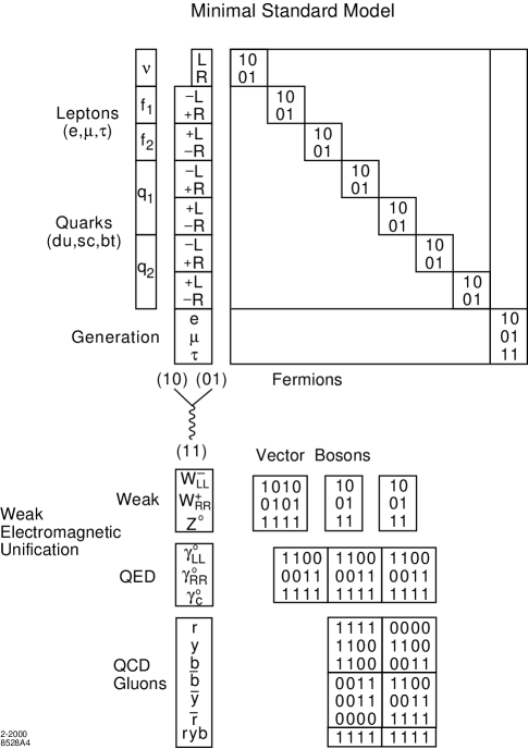
Figure 7: Skeleton of a label scheme for labels of length 16 which conveys the same quantum number information as the standard model of quarks and leptons.

References

- [1] T. Bastin, “On the Scale Constants of Physics”, Studia Philosophica Gandensia, 4, 77 (1966).
- [2] T. Bastin, H. P. Noyes, J. Amson and C. W. Kilmister, Int’l. J. Theor. Phys., 18, 445-488 (1979).
- [3] E. D. Jones, private communications to HPN starting in 1997; this fact, and a seminar on the type Ia supernovae data by Goldhaber at SLAC were primary motivations for HPN to attend DM98 and make the presentation already cited[14] that summer at ANPA20 (Sept., 1998).
- [4] J. Glanz, Science, 280, 1008, 15 May 1998.
- [5] J. Glanz, Science, 282, 1247, 13 September 1998.
- [6] D. E. Groom, et al., “Astrophysical Constants”, in [19], p.70.
- [7] C. J. Hogan, “The Hubble Constant”, in [19], pp 122-124.
- [8] C. H. Lineweaver, “A Younger Age for the Universe”, Science, 284, 1503-7 (1999).
- [9] M. J. Manthey, “Program Universe” in SLAC-PUB-4008, June 1986 (Part of Proc. ANPA 7), pp 101-110.
- [10] D. O. McGoveran, private communication to HPN November 19, 1998. McGoveran has tried to get this point across to this author, and to others committed to the ANPA research program, for several years.
- [11] H. P. Noyes, “Bit-String Physics, a Novel ‘Theory of Everything’ ”, in Proc. Workshop on Physics and Computation (PhysComp ’94), D. Matzke, ed.,94, Los Amitos, CA: IEEE Computer Society Press, 1994, pp. 88-94 and SLAC-PUB-6509. Aug 1994.
- [12] H.P.Noyes, “A Short Introduction to BIT-STRING PHYSICS”, in Merologies, Proc. ANPA 18, T.L.Etter, ed; [available from ANPA c/o K.Bowden, Theoretical Physics Research Unit, Birkbeck College, Malet St., London WC1E 7HX]; SLAC-PUB-7205, (June 1997) and hep-th 970702. This reference contains reasonably complete citations of the earlier literature.
- [13] See [12], Sect. 2, pp 28-32, for a brief discussion of program universe and a guide to the literature.
- [14] H. P. Noyes, “Program Universe and Recent Cosmological Results” SLAC-PUB-8030 (Jan 99), [gr-qc/9901022]; it also appeared in the Proceedings of the 20th annual meeting of the Alternative Natural Philosophy Association, Aspects II, K.G. Bowden, Ed. pp 192-214 [available from ANPA c/o K.Bowden, Theoretical Physics Research Unit, Birkbeck College, Malet St., London WC1E 7HX].
- [15] H.P.Noyes and E.D.Jones, “Solution of a Relativistic Three Body Problem”, Few Body Systems (in press) and SLAC-PUB-7609(rev), June 1998, and hep-th 971077.
- [16] H.P.Noyes and D.O.McGoveran, Physics Essays, 2, 76 1989), and SLAC-PUB-4528, Oct 1998.
- [17] K. A. Olive and D. N. Schramm(dec.), “Big-bang Nucleosynthesis”, in [19], pp 119-121.
- [18] K. A. Olive,“Big-bang Cosmology”, in [19], pp 117-118.
- [19] Particle Data Group, “Review of Particle Properties”, Phys.Euro. J. C 3, 1-794 (1998).
- [20] A. F.Parker-Rhodes, “Hierarchies of Descriptive Levels in Physical Theory”, Cambridge Language Research Unit, internal document I.S.U.7, Paper I, 15 January 1962; reprinted, together with comments by John Amson in K. Bowden, ed. Int.J. General Systems, 27 Nos. 1-3(1998), pp 57-80.
- [21] J. R. Primack, “Dark Matter and Structure Formation”, in Formation of Structure in the Universe, Proc. of the Jerusalem Winter School 1996, A. Dekel and J. P. Ostriker, eds. Cambridge University Press (in Press) and astro-ph/9797285v2 25 Jul 1997,