Systematic uncertainties in gravitational lensing models: a semi-analytical study of PG1115+080

Abstract

While the Hubble constant can be derived from observable time delays between images of lensed quasars, the result is often highly sensitive to assumptions and systematic uncertainties in the lensing model. Unlike most previous authors we put minimal restrictions on the radial profile of the lens and allow for non-elliptical lens potentials. We explore these effects using a broad class of models with a lens potential $\psi(rf(\theta))$, which has an unrestricted radial profile but self-similar iso-potential contours defined by $rf(\theta)=$ constant. For these potentials the lens equations can be solved semi-analytically. The axis ratio and position angle of the lens can be determined from the image positions of quadruple gravitational lensed systems directly, independent of the radial profile. We give simple equations for estimating the power-law slope of the lens density directly from the image positions and for estimating the time delay ratios. Our method greatly simplifies the numerics for fitting observations and is fast in exploring the model parameter space. As an illustration we apply the model to PG1115+080. An entire one-parameter sequence of models fit the observations exactly. We show that the measured image positions and time delays do not uniquely determine the Hubble constant.

1 Introduction

Gravitationally lensed systems are powerful probes of galactic potentials and the scale of the universe. The advantage over the traditional stellar dynamical method is that from the image positions we can measure the shape and the mass of the dark halo well beyond the half-light-radius of a faraway lens galaxy, whether it is virialized or not. The time delay between two images is a measurement of the difference in the length of the two bent light paths, and scales with the distances to the lens and source. So the Hubble constant can be constrained once the redshift of the lens and the source and the time delay are measured. This way of getting $H_{0}$ has the advantage that the underlying physics (general relativity) can be rigorously modeled. The limitation is that there is often a sequence of lens models that can fit the image positions.

Presently about twenty strongly lensed systems are known, half of them being quadruple-imaged quasars and half being double-imaged quasars (e.g., Keeton & Kochanek 1996). We will concentrate on quadruple-imaged systems. They are better constrained than double-imaged systems, since the lens model needs to fit more image positions and also the ratios of time delays between any two pairs of images. Quadruple systems typically involve a quasar source well-aligned with the center of the lens potential well. Presently only two such systems (PG1115+080 and B1608+656) have accurately determined image positions and time delays.

A significant amount of numerical computation is usually required to invert image positions to intrinsic parameters of the potential (cf. Schneider, Ehlers & Falco 1992). The degeneracy of the resulting potential is often not fully explored because of the need to cover a large parameter space, particularly for flattened potentials. Previous authors have often restricted their studies to isothermal or power-law spherical models (Evans & Wilkinson 1998 and references therein), and elliptical models (Witt & Mao 1997 and references therein) and other simple models (Kassiola & Kovner 1993, 1995) with or without external shear. The fully general non-parametric method, e.g., the pixelated lens method of Williams & Saha (2000), is very powerful in demonstrating the complete range of the degeneracy in the lens models, but it involves significant amount of numerical computation and does not provide a clear insight to the relations between the characteristic parameters of the lens. For these reasons it is still desirable to find analytical, yet general potentials, which allow a quick exploration of the model parameter space. For example, it is of interest to generalize the analytical work of Witt & Mao (1997) to non-elliptical lenses. It would also be interesting to find analytical expressions for the time delay in these general lenses, which could help us to understand how the radial profile and lens shape affect the predictions on the Hubble constant.

Here we study a broad class of analytical models with non-axisymmetric, non-elliptical shape and semi-power-law radial profile (§2), and show how to calculate the lens shape and radial profile parameters directly from the image positions (§3). We apply the models to PG1115+080 (§4) and show that the images can be fit perfectly by a large range of lens models (§5). We summarize our results in §6 and conclude with the implications on the Hubble constant.

2 Lens equation in a general class of models

2.1 Decoupling of angular dependence and radial profile

Any two-dimensional lens potential can be cast in the following form,

$$\psi(x,y)=\psi(\omega),~{}~{}~{}\omega=\omega(r,\theta),$$ (1)

where $\psi$ has the dimension of square arcsec, $(x,y)$ defines a rectangular coordinate system (in units of arcsecs to the West and North of the lens galaxy center) and $(r,\theta)$ the corresponding polar coordinate system with

$$(x,y)=(-r\sin\theta,r\cos\theta),$$ (2)

where $\theta$ is the position angle, counterclockwise from North. Unless otherwise specified we shall follow the notations of Schneider et al. (1992). Here $\omega$ is defined to have the dimension of radius, so that constant $\omega$ curves correspond to equal-potential contours, and define the shape and flattening of the potential. The radial profile of the potential is a smooth function $\psi(\omega)$ of the radius $\omega$. We can also define

$$m(\omega)\equiv\omega{d\psi\over d\omega}$$ (3)

as the mass (in units of square arcsec) enclosed inside the radius $\omega$ (in units of arcsec). For example, we have $m=\alpha\psi$ for a power-law model $\psi\propto\omega^{\alpha}$ with slope $\alpha$. For a source at redshift $z_{s}$ and angular distance $D_{os}(z_{s})$, and a lens at redshift $z_{l}$ and distance $D_{ol}(z_{l})$, the physical mass $M(\omega)$ is related to $m(\omega)$ by the scaling

$$M(\omega)\equiv\pi\Sigma_{c}~{}m(\omega),$$ (4)

where

$$\Sigma_{c}\equiv\frac{c^{2}}{4\pi G}\frac{D_{ol}D_{os}}{D_{ls}}\left(\frac{1~{}\rm radian}{206265~{}\rm arcsec}\right)^{2}\approx 39\frac{D_{ol}D_{os}}{D_{ls}}$$ (5)

is the critical density in units of $M_{\odot}/\rm arcsec^{2}$, and $D_{ls}(z_{l},z_{s})$ is the relative distance of the lens and source and all distances are in units of parsec.

A light ray from a source at $(r_{s},\theta_{s})$, being deflected to a direction $(r,\theta)$ by the lensing galaxy with potential $\psi(\omega)$ located at the origin, will experience a time delay $\Delta t$ given by

$$\Delta t(r,\theta)=h^{-1}\tau_{100}(z_{l},z_{s})\left[{1\over 2}r^{2}-rr_{s}\cos(\theta-\theta_{s})+{1\over 2}r_{s}^{2}-\psi(\omega)\right],$$ (6)

where $h$ is the Hubble constant $H_{0}$ rescaled to $100$ km/s/Mpc. A characteristic value for the time delay is

$$\tau_{100}(z_{l},z_{s})\equiv{D_{ol}D_{os}\over D_{ls}}{1+z_{l}\over c},~{}~{}~{}\mbox{for $H_{0}=100$~{}km/s/Mpc}.$$ (7)

According to Fermat’s principle, the images lie at the minimum of $\Delta t$, so the lens equation is given by

$${\partial\over\partial r}\Delta t = r-r_{s}\cos(\theta-\theta_{s})-m(\omega)\partial_{r}\ln\omega=0$$ (8)

$${\partial\over r\partial\theta}\Delta t = r_{s}\sin(\theta-\theta_{s})-{m(\omega)\over r}\partial_{\theta}\ln\omega=0.$$ (9)

Interestingly, the radial part $m(\omega)$ can be eliminated by simply combining the two equations,

$${r_{s}\sin(\theta-\theta_{s})\over r-r_{s}\cos(\theta-\theta_{s})}={\partial_{\theta}\ln\omega\over r\partial_{r}\ln\omega},$$ (10)

similar as in Witt & Mao (1997). This implies that there is a relation linking the image positions to the shape of the potential directly, independent of the radial profile.

2.2 Property of the image positions: the semi-hyperbolic curve

For simplicity we shall concentrate on self-similar models with

$$\omega(r,\theta)=r\cdot f(\theta),$$ (11)

where $f(\theta)$ defines the shape of the equal potential contours. In principle the shape function can be bi-symmetric or lopsided as long as the corresponding surface density is positive everywhere in the lens plane. To be specific, we will restrict our discussions to bi-symmetric potentials with an angular part

$$f(\theta)=\left|1-\delta\cos 2\theta^{\prime}\right|^{\beta},$$ (12)

which is a three-parameter $(\beta,\delta,\theta_{p})$ function of the angle $\theta$, where $\beta$ is a constant, the parameter $\delta$ is a flattening indicator, and $\theta_{p}$ is the position angle of a principal axis of the potential. The angle $\theta^{\prime}$ is the azimuthal angle $\theta$ except for a rotation with

$$\theta^{\prime}\equiv\theta-\theta_{p},~{}~{}~{}(x^{\prime},y^{\prime})=(r\cos\theta^{\prime},r\sin\theta^{\prime})$$ (13)

so that $(x^{\prime},y^{\prime})$ defines a rectangular coordinate system with the axes coinciding with the principal axes of the lens. For example, the source at

$$(x_{s},y_{s})=(-r_{s}\sin\theta_{s},r_{s}\cos\theta_{s})$$ (14)

in the original rectangular coordinate system would be at

$$(x^{\prime}_{s},y^{\prime}_{s})=(r_{s}\cos\theta^{\prime}_{s},r_{s}\sin\theta^{\prime}_{s}),~{}~{}~{}\theta^{\prime}_{s}\equiv\theta_{s}-\theta_{p},$$ (15)

in the rotated rectangular coordinate system.

With these we can compute the right-hand part of eq. 10,

$${\partial_{\theta}\ln\omega\over r\partial_{r}\ln\omega}={d\ln f(\theta)\over d\theta}={1\over v\cot\theta^{\prime}+u\tan\theta^{\prime}},$$ (16)

where

$$u\equiv{1+\delta\over 2\Delta},~{}~{}~{}v\equiv{1-\delta\over 2\Delta},~{}~{}~{}\Delta=2\beta\delta,$$ (17)

are shape indicators just like $\beta$ and $\delta$. Substituting in eq. 10, and rewriting the image radius $r$ as a function of $\theta^{\prime}$, we find the images fall on a family of curves $r=r(\theta^{\prime})$ defined by

$$r(\theta^{\prime})=r_{s}\left[\cos(\theta^{\prime}-\theta^{\prime}_{s})+\sin(\theta^{\prime}-\theta^{\prime}_{s})\left(v\cot\theta^{\prime}+u\tan\theta^{\prime}\right)\right].$$ (18)

An alternative expression for these curves can be obtained by expanding the sinusoidal terms in eq. 18 so that

$$r=(X_{a}\cos\theta^{\prime}+Y_{a}\sin\theta^{\prime})+\left({X_{b}\over\cos\theta^{\prime}}-{Y_{b}\over\sin\theta^{\prime}}\right),$$ (19)

which is now linear in four new parameters $(X_{a},Y_{a},X_{b},Y_{b})$; these parameters are related to the lens shape parameters $(v,u)$ and the source position $(x^{\prime}_{s},y^{\prime}_{s})$ by

$$X_{a}\equiv\left(1+v-u\right)x^{\prime}_{s},~{}~{}~{}Y_{a}\equiv\left(1-u+v\right)y^{\prime}_{s},~{}~{}~{}X_{b}\equiv ux^{\prime}_{s},~{}~{}~{}Y_{b}\equiv vy^{\prime}_{s}.$$ (20)

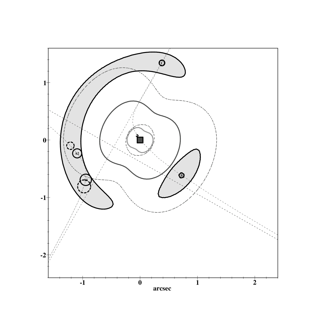
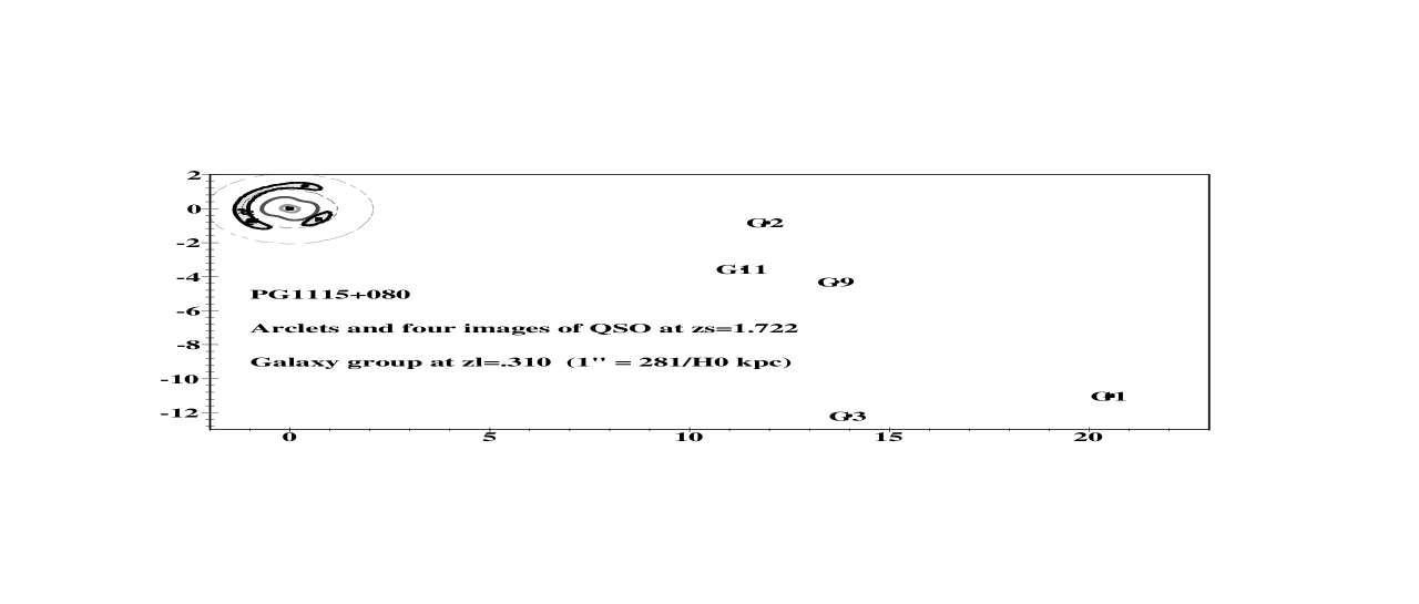
Figure 1: shows the relative locations of the four QSO images and the lens galaxy (filled square at the center) in the PG1115+080 system. The inset shows the relative locations of PG1115+080 and the neighbouring galaxies (G1 to G11 in the notation of Impey et al. 1998). The equation 18 for self-similar models also predicts a semi-hyperbolic curve passing through the observed images (solid circles), the predicted images (dashed circles) and the source (smaller half-closed circle) and the lens (the filled square) with asymptotic lines always being parallel to the symmetry axes of the potential. The area of the circles is in proportion to the flux. Overplotted are the predicted surface density contour maps (solid contours for density being 1 and 2 times the critical density) and critical curves (dashed contours) in the single-power-law model with $\beta=-{1\over 8}$. The nearly closed ring is predicted for a uniform disk around the QSO.

These curves (cf. eq. 18) have the nice property that they go through all image positions independent of the radial profile of the lensing galaxy. An example is the semi-hyperbolic curve in Fig. 1. The curve is determined by the source parameters $(r_{s},\theta^{\prime}_{s})$, the lens shape parameters $(v,u)$ and the lens position angle $\theta_{p}$. The radial profile can take any general physical profile, isothermal or power-law.

The boxiness parameter $\beta$ is such that the shape function $f(\theta)$ reduces to the usual elliptical form when $\beta={1\over 2}$ (Witt & Mao 1997). In the case that $\psi(\omega)$ is linear in $\omega$, the models reduce to the simple models of Kassiola & Kovner (1995) when $\beta=1$. Interestingly, elliptical models with $\beta={1\over 2}$ have $u-v={\delta\over\Delta}={1\over 2\beta}=1$ (cf. eq. 17), hence $X_{a}=Y_{a}=0$, and eq. 19 reduces to

$$1=\frac{X_{b}}{x^{\prime}}-\frac{Y_{b}}{y^{\prime}}$$ (21)

after applying $x^{\prime}=r\cos\theta^{\prime},y^{\prime}=r\sin\theta^{\prime}$. This equation prescribes a hyperbolic curve, which is consistent with Witt (1996) and Witt & Mao’s (1997) finding that all four image positions and the source position lie on a certain hyperbolic curve. A hyperbolic curve has a maximum of 5 free parameters, thus they cannot fit image positions of a general quadruple system; four image positions yield a minimal of eight constraints. Experience with fitting several quadruple systems (G2237+0305, CLASS1608+656, HST12531-2914) shows that models with $|\beta|\geq 1/2$ often give unphysical mass-radius relations $m(\omega)$. We find that $\beta=-{1\over 8}$ gives a fair approximation to realistic models. These models have non-elliptical contours, and often yield physical density distributions. Fig. 2 shows that they also cover a sufficiently wide range of axis ratios for the potential and the density so that we can explore the shape of the lens galaxy in fitting the image positions. The expressions for the axis ratios of a power-law lens are given in Appendix A.

3 Results

3.1 Lens shape directly from fitting image positions

Our models can be used to fit image positions and derive lens shape parameters ($\delta,\beta$) and the source position $(r_{s},\theta_{s})$, free from assumptions of the lens radial profile, but subject to the assumption that the lens’ angular profile obeyes eq. 12. The four unknowns can be derived from the four observed image positions, i.e., the eight observables $(r_{i},\theta_{i})$ with $i=1,2,3,4$. The position angle $\theta_{p}$ of the lens principal axis is treated as a free variable.

The procedure is simple. First substitute the four observed image positions in eq. 19 to obtain the following four linear equations

$$\frac{\cos\theta^{\prime}_{i}}{r_{i}}X_{a}+\frac{\sin\theta^{\prime}_{i}}{r_{i}}Y_{a}+\frac{1}{r_{i}\cos\theta^{\prime}_{i}}X_{b}-\frac{1}{r_{i}\sin\theta^{\prime}_{i}}Y_{b}=1,~{}~{}~{}i=1,2,3,4,$$ (22)

of the four unknown parameters $(X_{a},Y_{a},X_{b},Y_{b})$. After solving these, either analytically or numerically, these parameters are substituted in eqs. 20, 15, and 17 to yield the source position and the lens shape in terms of $(r_{s},\theta_{s},\delta,\beta)$. In fact, we can recast eq. 20 to a set of four simple linear equations of four new unknowns $(u,v,1/x^{\prime}_{s},1/y^{\prime}_{s})$ by moving the terms $x^{\prime}_{s}$ and $y^{\prime}_{s}$ to the left hand side of the equations, i.e.,

$$X_{a}/x^{\prime}_{s}-v+u=1,~{}~{}~{}Y_{a}/y^{\prime}_{s}-v+u=1,~{}~{}~{}X_{b}/x^{\prime}_{s}-u=0,~{}~{}~{}Y_{b}/y^{\prime}_{s}-v=0.$$ (23)

The lens shape parameters $(\delta,\beta)$ can then be computed from

$$\delta=\frac{u-v}{u+v},~{}~{}~{}\beta=\frac{1}{2(u-v)},$$ (24)

and the source position $(r_{s},\theta_{s})$ from

$$r_{s}=\sqrt{{x^{\prime}_{s}}^{2}+{y^{\prime}_{s}}^{2}},~{}~{}~{}\theta_{s}=\arctan(y^{\prime}_{s},x^{\prime}_{s})+\theta_{p}.$$ (25)

Thus we have effectively reduced the problem of fitting image positions to successively solving linear equations, which is a straightforward task.

3.2 Non-parametric radial profile and power-law slope

The radial part of the potential can also be extracted from eq. 8 without parameterization. At the positions of the images we have

$$m(\omega)=r^{2}-rr_{s}\cos(\theta-\theta_{s})=x^{2}+y^{2}-xx_{s}-yy_{s},~{}~{}~{}\omega=rf(\theta),$$ (26)

where we have used $\partial_{r}\ln\omega=r^{-1}$. Thus we have obtained a mass-radius relation directly from the observed image positions, assuming that the source position $(x_{s},y_{s})$ and the flattening and position angle of the potential $(\delta,\theta_{p})$ have been determined by fitting the curve (cf. eq. 18). Interestingly, in the limit that the source is at the center of a circular lens, we have $r_{s}\rightarrow 0$, $\beta\rightarrow 0$ and $m\rightarrow r^{2}$.

It is useful to characterize the radial profile of a lens galaxy, which is generally not a power-law, by an effective power-law slope $\alpha(\omega)$, which varies with the radius $\omega$ except for scale-free models. There are several ways of estimating the characteristic power-law slope. Taking any two images $i$ and $j$, we can form a characteristic power-law slope $\alpha_{ij}$ from the mass $m_{i}$ and $m_{j}$ at the image radii $\omega_{i}$ and $\omega_{j}$ with

$$\alpha_{ij}\equiv{\log m_{i}-\log m_{j}\over\log\omega_{i}-\log\omega_{j}}={2\log{r_{i}\over r_{j}}+\log{1-r_{s}r_{i}^{-1}\cos(\theta_{i}-\theta_{s})\over 1-r_{s}r_{j}^{-1}\cos(\theta_{i}-\theta_{s})}\over\log{r_{i}\over r_{j}}+\beta\log{1-\delta\cos(\theta_{i}-\theta_{s})\over 1-\delta\cos(\theta_{j}-\theta_{s})}},$$ (27)

where we have used the mass-radius eq. 26.

Alternatively we can estimate the power-law slope from the observed time delay. First we rewrite the time delay eq. 6, so that the time delay, $t_{ij}$, between any two images $i$ and $j$ is given by

$${ht_{ij}\over\tau_{100}}={1\over 2}(x_{i}^{2}+y_{i}^{2})-{1\over 2}(x_{j}^{2}+y_{j}^{2})-(x_{i}-x_{j})x_{s}-(y_{i}-y_{j})y_{s}-(\psi_{i}-\psi_{j}),$$ (28)

where $\psi_{i}-\psi_{j}$ is the difference in the lens potential between the two images. Rewriting eq. 28 we form a new estimator $\alpha^{t}_{ij}$ for the power-law slope with

$$\alpha^{t}_{ij}\equiv{m_{i}-m_{j}\over\psi_{i}-\psi_{j}}={(x_{i}^{2}+y_{i}^{2})-(x_{j}^{2}+y_{j}^{2})-(x_{i}-x_{j})x_{s}-(y_{i}-y_{j})y_{s}\over{1\over 2}(x_{i}^{2}+y_{i}^{2})-{1\over 2}(x_{j}^{2}+y_{j}^{2})-(x_{i}-x_{j})x_{s}-(y_{i}-y_{j})y_{s}-{ht_{ij}\over\tau_{100}}},$$ (29)

where we have used eq. 26.

Thus we have two direct estimators $\alpha_{ij}$ and $\alpha^{t}_{ij}$ of the radial profile, computed from the observed images and time delays. In the limit of scale-free power-law models $\alpha_{ij}=\alpha^{t}_{ij}=\alpha(\omega)=cst$. So the deviation from scale-freeness can be estimated by taking the differences such as $\alpha_{12}-\alpha_{34}$, $\alpha^{t}_{12}-\alpha^{t}_{34}$, or $\alpha_{14}-\alpha^{t}_{14}$.

3.3 Hubble constant and time delay ratios

To apply the above estimates of the power-law slopes, we have assumed that we know the rescaled Hubble constant $h$ from independent observations. Alternatively the Hubble constant $H_{0}=100h$ can be estimated from the time delay $t_{ij}$ between two images. Letting $\alpha^{t}_{ij}=\alpha_{ij}$, we get

$$h={\tau_{100}\over t_{ij}}\left\{\left({1\over 2}-{1\over\alpha_{ij}}\right)\left[(x_{i}^{2}+y_{i}^{2})-(x_{j}^{2}+y_{j}^{2})\right]-\left(1-{1\over\alpha_{ij}}\right)\left[(x_{i}-x_{j})x_{s}+(y_{i}-y_{j})y_{s}\right]\right\}.$$ (30)

The time delay ratio can also be predicted with

$${t_{ij}\over t_{kl}}={\left({1\over 2}-{1\over\alpha_{ij}}\right)\left[(x_{i}^{2}+y_{i}^{2})-(x_{j}^{2}+y_{j}^{2})\right]-\left(1-{1\over\alpha_{ij}}\right)\left[(x_{i}-x_{j})x_{s}+(y_{i}-y_{j})y_{s}\right],\over\left({1\over 2}-{1\over\alpha_{kl}}\right)\left[(x_{k}^{2}+y_{k}^{2})-(x_{l}^{2}+y_{l}^{2})\right]-\left(1-{1\over\alpha_{kl}}\right)\left[(x_{k}-x_{l})x_{s}+(y_{k}-y_{l})y_{s}\right]},$$ (31)

which is obtained by rewriting eq. 30.

4 Application: the surface density and time delay models for PG1115+080

4.1 Data

As a simple application, we model the image positions and time delays of the well-studied quadruple system PG1115+080. This system has been extensively studied ever since the first models by Young and collaborators (1981), and has received closer attention after Schechter et al.’s (1997) measurements of its time delay. All models, except those of Saha & Williams (1997), adopt elliptical/circular shapes and a few common radial profiles, with the models of Keeton & Kochanek (1997) and Impey et al. (1998) being the most comprehensive. Only one year after the discovery of the legendary double-image radio-loud quasar Q0957+561, this system was identified as a multiple-imaged system by Weymann et al. (1980) in their survey of nearby bright QSOs. It is now known to consist of four images with the names $A_{1}$, $A_{2}$, $B$ and $C$ (with flux ratios about 4 : 2.5 : 0.7 : 1, cf. the HST observations of Kristian et al. 1993) of a radio-quiet QSO at redshift $z_{s}=1.722$. The images $A_{1}$ and $A_{2}$ are within $0.5^{\prime\prime}$; see the inset of Fig. 1. Interestingly, the lens galaxy is also one of the bright members of a galaxy group ($N\sim 10$) at redshift $z_{l}=0.310$, first mapped by Young et al. (1981). The center of the group is to the south-west of the lens, roughly at $r_{g}=(20^{\prime\prime}\pm 2^{\prime\prime})$ and $\theta_{g}=(-117^{o}\pm 3^{o})$. The lens galaxy has been resolved by both HST and the 8.2-m Subaru telescope in $0.3^{\prime\prime}$ seeing. It appears to be an early type galaxy with a de Vaucouleurs profile and a half-light radius of $0.55^{\prime\prime}$. There is no sign of differential dust-extinction in the lens galaxy. While NICMOS observations by Impey et al. (1998) show no flattening for the lens, ground infrared images by Iwamuro et al. (2000) found it to be an E1 galaxy elongated towards $\theta_{p}\sim 65^{o}$. Both observations reveal a $1^{\prime\prime}$ infrared Einstein ring connecting the four images, which is thought to be the infrared image of the QSO host galaxy. PG1115+080 is also one of the two quadruple systems where the time delay between images has been measured, the other one being the radio-loud quasar B1608+656 from the CLASS survey (cf. Fassnacht et al. 1999). Although two different sets of values are quoted in the literature (Schechter et al. 1997, Barkana 1997), the leading image is the furtherest image (the image C), and the innermost image (image B) arrives last. The time delay ratio $r_{ABC}=t_{AC}/t_{BA}$, for the delay between image $C$ and $A_{1}+A_{2}$ vs. image $B$ and $A_{1}+A_{2}$, provides an extra discriminator of the models; the images $A_{1}$ and $A_{2}$ are within $0.5^{\prime\prime}$ of each other, and the small relative delay is undetected. Schechter et al. first reported $r_{ABC}=0.7\pm 0.3$ from their photometric monitoring program in 1995-1996. Later analysis by Barkana (1997) found $r_{ABC}=1.13\pm 0.18$, after taking into account correlations of errors amongst the time delays. The delay between images B and C, $t_{BC}=25.0\pm 1.7$ days.

Here we illustrate the application of our models to the most recent data from Impey et al. (1998) of PG1115+080. We do not attempt to model B1608+656 because the lens appears to be a merging pair of galaxies, and the morphology is too complex for our model. We denote with the index $i=1,2,3,4$ the four images $A_{1}$, $A_{2}$, $B$ and $C$. All results are quoted for a standard flat universe without a cosmological constant $(\Omega,\Lambda)=(1,0)$. Table 1 gives the relevant quantities to calibrate our results to other universes. The angular distance from redshift $z_{1}$ to $z_{2}$ in a universe of a matter and vacuum density $(\Omega,\Lambda)$ times the closure density is generally given by

$$D(z_{1},z_{2})={c\over H_{0}(1+z_{2})\sqrt{\Omega_{c}}}\sinh\left\{\sqrt{\Omega_{c}}\int_{z_{1}}^{z_{2}}dz\left[\Lambda+\Omega_{k}(1+z)^{2}+(1+z)^{3}\Omega\right]^{-{1\over 2}}\right\},~{}~{}\Omega_{k}=1-\Lambda-\Omega.$$ (32)

The predicted Hubble constant should be reduced from the value achieved with the standard $(\Omega,\Lambda)=(1,0)$ universe by 3% in the presently favored $\Lambda$-dominated universe with $(\Omega,\Lambda)=(0.3,0.7)$ from surveys of distant supernovae.

4.2 The source position, the lens shape and mass inside images

First we solve for the lens shape and source position from the linear equations  19 and 23. The solutions for PG1115+080 are given in Table 2, sorted according to the value of $\beta$ or $\theta_{p}$. The resulting potential model with $\beta=-{1\over 8}$ or $\theta_{p}=60.5^{\circ}$ has a flattening of between E0 and E1, and interestingly the lens principal axis points towards the location of the galaxy group in the lens plane. Models with other values of $\beta$ or $\theta_{p}$ will be discussed in section 5.

To proceed with determining the lens mass at each image position, we substitute the now known flattening parameters $(\delta,\theta_{p})$ and the source positions $(r_{s},\theta_{s})$ in eq. 26, to predict four independent data points $(\omega_{i},m_{i})$ with $i=1,2,3,4$ in the radius vs. the enclosed mass plane. Fig. 3 shows the predicted lens mass enclosed at the four image positions. Note that the mass rises faster than the light, implying a growing dark mass component at large radius; the light distribution is modeled as an observed de Vaucouleurs $r^{{1\over 4}}$-law with a half-light radius of $0.55^{\prime\prime}$.

4.3 Piecewise power-law model

So far we did not enforce any strict parameterization of the radial profile. We only restrict the profile to be of the form of eq. 11; in practice, this is an insignificant restriction. In the following sections we show several ways of modeling the radial profile assuming an isolated lens. None of the models is completely satisfactory.

First we use a minimal model, which assumes that the mass-radius relation is a piecewise power-law, that is, we connect a straight line through two images in the $\log m$ vs. $\log\omega$ plane. The piecewise values for the power-law slope and axis ratios are given in Table 2.

The Hubble constant $H_{0}=100h$ can be estimated by normalizing the time delay to the observed value $t_{AC}$ (Schechter et al. 1997),

$$h={\tau_{100}\over 2t_{AC}}\left[-P_{14}+\left(1-{1\over\alpha_{14}}\right)S_{14}\right],$$ (33)

where

$$P_{ij}=\left[(x_{i}^{2}+y_{i}^{2})-(x_{j}^{2}+y_{j}^{2})\right]$$ (34)

depends on the image positions $(x_{i},y_{i})$ alone and

$$S_{ij}=2P_{ij}-2\left[(x_{i}-x_{j})x_{s}+(y_{i}-y_{j})y_{s}\right]$$ (35)

depends on the source position $(x_{s},y_{s})$ as well. The model yields a Hubble constant $H_{0}\sim 30$ km/s/Mpc, much lower than determined by other authors (e.g., Impey et al. 1998). The low $H_{0}$ is a result of the high value for the power-law slope $\alpha_{AC}=1.6$. Other values are given in Table 2 for various image pairs and observed time delay. The time delay ratio can also be predicted with (cf. eq. 31)

$$r_{ABC}\equiv{t_{14}\over t_{32}}={-P_{14}+\left(1-{1\over\alpha_{14}}\right)S_{14}\over-P_{32}+\left(1-{1\over\alpha_{32}}\right)S_{32}}.$$ (36)

Substituting the slopes $\alpha_{AC}$ and $\alpha_{BA}$ to eq. 31 we find the ratio between images $r_{ABC}=t_{AC}/t_{BA}\sim 0.65$.

Note that the time delay predictions here are robust and independent of details of the density, since the discontinuity in the density is completely smoothed out in the lensing potential.

4.4 Single power-law model

The piecewise-power-law model above necessarily implies a discontinuous density profile. This could be cured if we enforce a single power-law model, that is, we fit a straight line to the four points in the $\log m$-$\log\omega$ plane. This would give us a power-law slope $\alpha=1.38$. Fig. 1 shows our model surface density contours. Similar to the non-parametric models of Saha & Williams (1997) we find a peanut-shaped lens.

We can estimate the goodness of the fit by recomputing the image positions from a given mass model. The general procedure of simulating images of our theoretical lens model is as follows: First combine eq. 26 with the power-law radial profile to get

$$r^{2}-rr_{s}\cos(\theta-\theta_{s})=m(\omega)=b_{0}r_{0}\left({\omega\over r_{0}}\right)^{\alpha},~{}~{}~{}\omega=r\left|1-\delta\cos(2\theta-2\theta_{p})\right|^{\beta}.$$ (37)

Then upon substitution of eq. 18 to eliminate $r$, we obtain a one-dimensional non-linear equation for the image position angle $\theta$, which can be solved easily numerically. As a comparison, one would be dealing with a minimum-finding or a root-finding numerical problem in a two-dimensional plane $(r,\theta)$ in the general case without the separation of the angular vs. radial part. For our model of PG1115+080, the image solutions are shown in Fig. 1 as dashed circles, together with the input observed image positions (solid circles). The predicted four images are off by about 60 milli arcsecs, a residual which is inconsistent with the $\sim 3$ milli arcsecs accuracy of Impey et al. positions, and is marginally consistent with earlier data by Kristian et al. with a quoted error of 50 milli arcsec for the lens galaxy and 5 milli arcsec for the images. The images $A_{1}$ and $A_{2}$ are at two sides of the critical curve (the line of infinite amplification in the source plane), hence are highly amplified with opposite parity. The time delay ratio can be estimated with eq. 31, assuming a constant power-law slope $\alpha=\alpha_{BC}=1.38$. This yields $r_{ABC}\sim 1.3$, close to the Barkana (1997) value of $1.13\pm 0.18$. The large difference here is due to the large residual in terms of fitting the images $A_{1}$ and $A_{2}$ with a straight power-law.

We also compute the amplification patterns by taking double derivatives of the time delay surface. The circles in Fig. 1 show the observed (solid circles) and predicted (dashed circles) fluxes of each image and the source (half-closed circle), with the area of each circle in proportion to the flux. The $B$ to $C$ ratio is well-reproduced and the predictions for images $A_{1}$ and $A_{2}$ are also consistent with observations at about the 0.3 magnitude level.

Finally, if we put a host galaxy around the QSO, the model predicts that the image of the host galaxy will be stretched into an arc. We see a nearly closed ring. This agrees very well with the diffuse ring that Impey et al. discovered in their NICMOS images. The ring maps back to the source plane as a disk with an area of $\sim 0.03$ square arcsec.

4.5 Double power-law model

Alternatively we can fit a smooth, five-parameter lens model with a lens potential

$$\psi(\omega)=c_{0}\left({\omega\over a_{0}}\right)^{\alpha_{in}}\left[1+\left({\omega\over a_{0}}\right)^{n}\right]^{\alpha_{out}-\alpha_{in}\over n},~{}~{}~{}\omega=r\left|1-\delta\cos(2\theta-2\theta_{p})\right|^{\beta}.$$ (38)

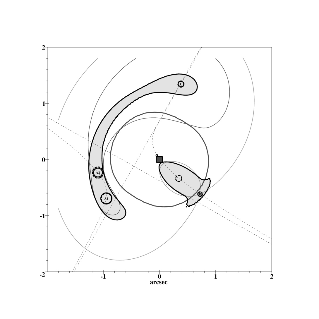
Figure 4: Similar to Fig. 1, but for the double-power-law model with $\beta=-{1\over 8}$. Overplotted is a solid contour, showing the predicted surface density at the critical density. Also shown is the predicted time delay “finger print” for the double-power-law model with $\beta=-{1\over 8}$. The contour passing close to the separatrix (image $B$) is split to two disconnected contours. The extra fifth image (the isolated dashed circle near the image B) is a result of the non-monotonic model density, and it sits on a local extreme of the delay contour. The other contour is a contour of constant time delay ratio $t_{XC}/t_{BX}=0.7$ of any point $X$ and images $B$, $C$.

The corresponding mass profile is given in Appendix B. This model assumes the lens potential (as well as the lens mass) increases like a double-power-law with an inner slope $\alpha_{in}$ and outer slope $\alpha_{out}$. The transition is defined by the normalization constant $c_{0}$, the radius $r=a_{0}$ and the sharpness parameter $n$; bigger $n$ corresponds to sharper transition. When fitting the mass model to the four points in Fig. 3, it turns out that the inner slope $\alpha_{in}$ is fully unconstrained. The other four free parameters $(c_{0},a_{0},\alpha_{out},n)$ are determined from fitting the four data points; the procedure is explained in Appendix B. The values of $(c_{0},a_{0},\alpha_{out})\sim(0.6,1.1,1.63)$, nearly independent of the value for the inner slope $\alpha_{in}$. Note $\alpha_{out}\sim\alpha_{AC}$, consistent with the fact that the mass at $A_{1}$, $A_{2}$ and $C$ follows nearly a power-law (cf. Fig. 3). The value of $n$ increases from $\sim 15$ to $\sim 39$ for $\alpha_{in}=0-2$. That $n\gg 2$ means that the density changes sharply at the transition. All fits have zero residual and predict nearly identical mass profiles at radii between images $B$ and $C$. They differ only in the mass profile inside image $B$, where we have no direct constraint on the dark matter profile. For all purposes it is sufficient to set $n=20$ so that $\alpha_{in}\sim 2$, in which case the model has a finite core at small radii. From the potential model we can compute the dimensionless surface density contours (cf. Fig. 4). Near the position of the images, the density has a flattening of E2-E3, flatter than the potential, as expected. The potential model can also be substituted in eq. 6 to predict the time delay contours, shown in Fig. 4. The observed images $C$, $A_{2}$, $A_{1}$, $B$ (the solid circles) are exactly the valley, peak, saddle, valley points of the delay contour, where the theoretical images should lie according to Fermat’s principle. The images $A_{1}$ and $A_{2}$ have nearly the same arrival time. Substituting the lens potential in eq. 28 we can predict the time delay ratio for the double-power-law model. The result, $r_{ABC}\sim 0.65$, is nearly the same as the piece-wise power-law model. These predicted ratios are in good agreement with the earlier measurement of $0.7\pm 0.3$ of Schechter et al. (1997).

We can recompute the image positions from the double-power-law model by solving

$$r^{2}-rr_{s}\cos(\theta-\theta_{s})=m(\omega)=c_{0}\left({\omega\over a_{0}}\right)^{\alpha_{in}}\left[1+\left({\omega\over a_{0}}\right)^{n}\right]^{\alpha_{out}-\alpha_{in}\over n},~{}~{}~{}\omega=r\left|1-\delta\cos(2\theta-2\theta_{p})\right|^{\beta},$$ (39)

and eq. 18.

Unlike the single-power-law model it predicts five images (cf. Fig. 4). Four predicted images fall exactly on the observed positions. But the model predicts an extra image near image B. This can be identified with the usually highly demagnified fifth image that is sometimes observed in lensed systems. The extra image the model predicts is, however, too bright to be consistent with observations. This is a direct consequence of the fact that $\kappa$ at its radius is nearly constant and $\sim 1$. The amplification can be calculated from $\kappa$ as $(1-\kappa)^{-2}\sim 25$.

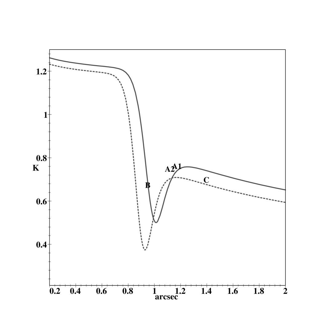
Figure 5: The predicted run of the dimensionless density $\kappa$ along (solid) and perpendicular to (dashed) the principal axis $\theta_{p}=60.5^{o}$ (i.e. $\beta=-{1\over 8}$) for the double-power-law model. The model is positive everywhere, but has a peculiar wiggle at about $1^{\prime\prime}$.

All images lie on the curve defined by eq. 18. The extra image arises because the model density profile (cf. Fig. 5) is non-monotonic near $1^{\prime\prime}$ radius, the transition radius $a_{0}$ of the double-power-law potential model. A wiggle in density happens when the transition parameter $n>2$, i.e., a sharp transition of the potential.

5 Discussion

5.1 Power-law slope of PG1115+080 vs. $H_{0}$ and time delay ratio

The previous sections have illustrated the procedure for fitting known quadruple image systems with our models, and have also revealed some puzzling problems with PG1115+080, for example, the low and non-unique $H_{0}$ and the peculiar and non-unique lens density. Fig. 6 shows the values for $\alpha$ predicted from either the mass-radius relation (cf. eq. 27) or from the time delay (cf. eq. 29). Two comments are in order: (1) There is a large spread with the power-law slope $\alpha$ depending on how it is predicted. To fit the observed time delay within $2\sigma$ with a reasonable $H_{0}$ (between 50 and 100 km/s/Mpc), we obtain only a loose constraint $0.3<\alpha<1.6$. (2) The rise of the power-law slope $\alpha$ with radius in the piecewise-power-law model is somewhat unphysical; realistic models typically have a monotonically steeper density profile (smaller $\alpha$) with increasing radius. These results are consistent with the finding of a wiggle near the transition radius ($1^{\prime\prime}$) in the surface density of the smooth double-power-law fits. Nevertheless the density is positive everywhere.

A detailed treatment of these problems should include the effect of the neighboring group. Such models are presented elsewhere, since they are beyond the interest of this paper on methods for quadruple systems in general. Nevertheless some further study of the model parameter space is clearly needed. Here it is sufficient to comment on the range of the predicted model parameters, in particular, the power-law slope and the value of $H_{0}$ when we vary the parameter $\beta$ or $\theta_{p}$.

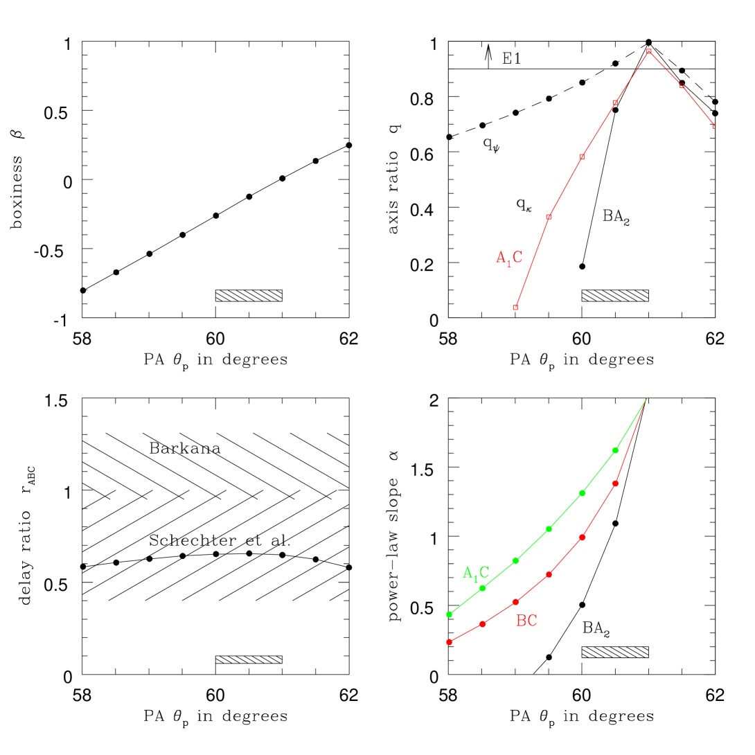
Figure 7: The parameter space of the isolated lens model. The four panels show (in clockwise direction) the model boxiness parameter $\beta$, the axis ratio $q_{\psi}$ of the potential and $q_{\kappa}$ of the density (cf. eq. 47 and eq. 48), the power-law slope $\alpha$ (cf. eq. 27), and the delay ratio $r_{ABC}$ (cf. eq. 31). The shaded bar at the bottom of each panel indicates the range of physically allowed models.

Fig. 7 shows the parameter space of the isolated lens model by varying the orientation of the lens principal axis $\theta_{p}$ (cf. eq. 12 and 13). It turns out a one-parameter family of models fits the observations; we effectively vary $\beta$. In fact, $\theta_{p}\sim 61^{o}+4\beta$, and $\Delta=2\beta\delta\sim{\beta\over 2}$ to a fair accuracy. We find that models with $\beta<-1/3$ will generally result in negative density models, models with $\beta\geq 0$ have a radially-increasing density, and models with $|\beta|\rightarrow 0$ also produce a nearly constant axisymmetric density, hence implying an unphysically small Hubble constant. Only in the range $-{1\over 4}\leq\beta<0$ do we find physical models with a reasonable flattening. The source positions for different models are shown in Fig. 8. Table 2 compares the predicted parameters of the $\beta=-{1\over 4}$ or $\theta_{p}=60^{\circ}$ model with the $\beta=-{1\over 8}$ or $\theta_{p}=60.5^{\circ}$ model. Fig. 3 shows the predicted radial profile for both models. Both models would have a significant residual if we fit the image positions with a straight power-law, or strange wiggles and extra images if we fit a double-power-law. We find this is generally the case with all isolated lens models without the shear from the neighbouring group.

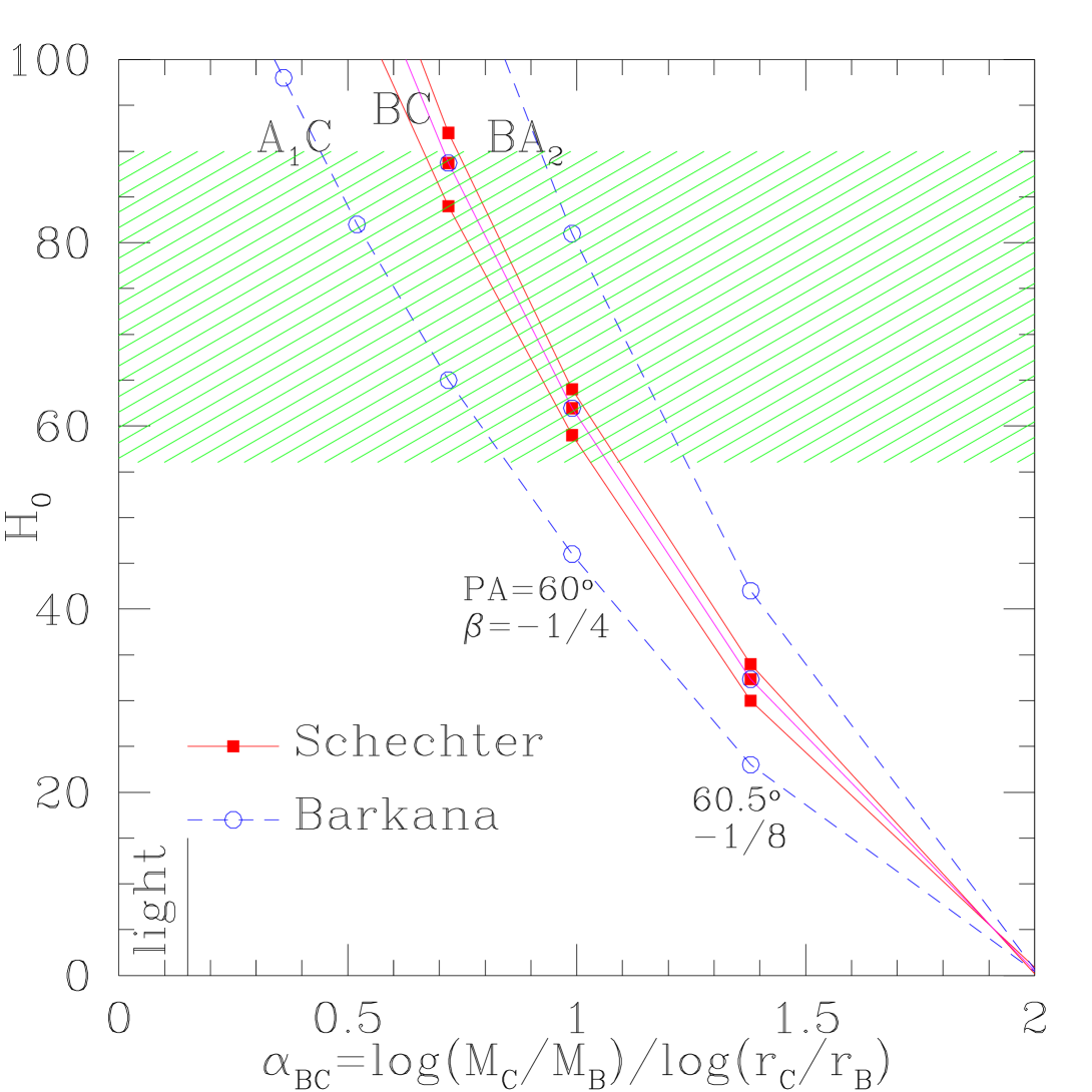
Figure 9: The dependence of $H_{0}$ on the power-law slope $\alpha$, where $\alpha$ is determined by the ratio of increase in mass and increase in distance. The short vertical line to the left shows the slope of increase in light $\log(L_{C}/L_{B})/\log(r_{C}/r_{B})$. The curves show the predictions for $H_{0}$ using $t_{AC}$, $t_{BC}$, and $t_{BA}$ measured by Schechter et al. (1997), solid line, and Barkana (1997), dashed line. The shaded region shows the consensus value for $H_{0}$.

Fig. 9 shows that there is significant degeneracy with the value for $H_{0}$, depending on the adopted model and the adopted time delay. The most reliable estimate is from the delay between the innermost image B and the outermost image C using

$$h={\tau_{100}\over 2t_{BC}}\left[-P_{14}+\left(1-{1\over\alpha_{14}}\right)S_{14}-P_{32}+\left(1-{1\over\alpha_{32}}\right)S_{32}\right],$$ (40)

where we neglected the time delay between the images $A_{1}$ and $A_{2}$. The $H_{0}$ thus predicted scales approximately as $60(2-\alpha)$ km/s/Mpc (cf. Fig. 9), where $\alpha=\alpha_{BC}$ is the average power-law slope. The factor $2-\alpha$ is the average power-law slope of the model surface density, and is not well-constrained at the radius of the images. Models with $\beta\sim-{1\over 4}$ or $\theta_{p}=60^{\circ}$ predict a steeper density profile, and closer to isothermal than models with $\beta\sim-{1\over 8}$ or $\theta_{p}=60.5^{\circ}$, hence yield a more plausible $H_{0}$ around $60$ km/s/Mpc. Models with very shallow profiles ($\alpha>1$) are unfavored by the consensus value for $H_{0}$.

In all our isolated lens models, the delay ratio is closer to the Schechter value, while the Barkana value seems to be the widely accepted one. This explains why we see in Fig. 9 a tighter prediction of $H_{0}$ using $t_{AC}$ and $t_{BA}$ of Schechter values than the Barkana values. Interestingly in the limit that the isothermal model is applicable, $\alpha=1$, the time delay ratio can be estimated from the image positions directly (i.e. without computing the source position) with the following equation:

$$r_{ABC}={P_{14}\over P_{32}}={r_{1}^{2}-r_{4}^{2}\over r_{3}^{2}-r_{2}^{2}}\sim 0.65,~{}~{}~{}\mbox{\rm for isothermal lens},$$ (41)

where $r_{i}$ is the observed radius of the image $i$ from the lens center. The ratio increases when we introduce the shear from the nearby group.

5.2 Rotation curve and mass-to-light ratio

Fig. 10 compares the predicted velocity dispersion for the lens with the observed value. The dispersion is predicted with the following formula,

$$\sigma_{i}^{2}=V^{2}{m_{i}\over 2r_{i}},~{}~{}~{}V^{2}\equiv{D_{os}\over D_{ls}}{(3\times 10^{5}{\rm km/s})^{2}\over 2\pi~{}{\rm radian}}{1~{}{\rm radian}\over 206265~{}{\rm arcsec}},$$ (42)

where the predictions are made from each image $i=1,2,3,4$ (strictly speaking the formula is valid only for a singular isothermal lens). Applying this for each value of the lens position angle $\theta_{p}$ we get the full range of possible values for the dispersion. The difference of the dispersion among the four images shows the deviation from an isothermal model. On average the predicted lens galaxy velocity dispersion, 200-300 km/s, suggests that the lens is close to a massive $L_{*}$ galaxy. The observed dispersion $\sigma=(281\pm 50)$ km/s ($95\%$ confidence, shaded region) from the Keck spectrum of Tonry (1998). This value is comparable to the theoretical models, but on the high side. A similar problem has been noted in previous models (Schechter et al. 1997). Tonry noted that the discrepancy might be due to a steep radial fall-off of the velocity dispersion or a simple over-estimation of the observed dispersion; the spectrum of the faint lens was made from subtracting two Keck spectra taken with a $1^{\prime\prime}$-slit, one passing the lens and the image B, one passing the images $A_{1}$ and $A_{2}$.

Fig. 11 compares the increase of the lens mass from the innermost image $B$ to the outermost image $C$ vs the increase of the lens light. The mass ratio is predicted using

$${M_{C}\over M_{B}}={m_{4}\over m_{3}}=\left({r_{4}\over r_{3}}\right)^{\alpha_{BC}}.$$ (43)

where the power-law slope $\alpha_{BC}$ depends the principal axis $\theta_{p}$. The light ratio

$${L_{C}\over L_{B}}={\int_{0}^{r_{4}}dr2\pi r\exp\left[-7.67\left({r\over r_{e}}\right)^{1\over 4}\right]\over\int_{0}^{r_{3}}dr2\pi r\exp\left[-7.67\left({r\over r_{e}}\right)^{1\over 4}\right]},~{}~{}~{}r_{e}=0.55^{\prime\prime},$$ (44)

where the observed de Vaucouleurs law is used for the projected light. The fact that ${M_{C}\over M_{B}}>{L_{C}\over L_{B}}>1$ implies that the mass grows faster than the light at these radii for all these models, consistent with a large amount of dark matter between 0.8 and 1.5 arcsec.

6 Conclusion

Here we itemize our main results.

(i) We found a very general class of lens models that allow for non-elliptical and non-scale-free lenses. These models include previous isothermal elliptical models as special case. We can derive the radial mass distribution of the lens in a non-parametric way. We can study the deviation from the usually assumed straight power-law profile. We also give simple formulas for computing the time delay ratios and for estimating $H_{0}$.

(ii) The models are very easy to compute and can be used for efficient exploration of a large parameter space because the lens equations can be reduced to a set of linear equations.

(iii) We have applied the models to PG1115+080, and have explored a large parameter space of isolated lens models. All models using piece-wise-power-law or double-power-law fit the positions of the images exactly. The models can also reproduce the flux ratios between the images and the stellar velocity dispersion of the lens approximately.

(iv) Our models are consistent with a dark halo up to a radius of three times the half-light-radius of the lens. The enclosed mass increases much faster than the enclosed light as we move radially from the innermost image to the outermost image.

(v) We reconfirm earlier results by (e.g. Schechter et al. 1997) that the principal axis of the lens potential points, within a few degrees, to the external group, and is consistent with the observed value (Iwamuro et al. 2000).

(vi) Our models do not yield a unique prediction of $H_{0}$, because it is sensitive to the lens power-law slope $\alpha$ (cf. Fig. 9), which appears to have a large spread, depending on how it is predicted. The power-law slope is also sensitive to small uncertainties of the position angle of the lens $\theta_{p}$. A change of $\theta_{p}$ by a few degrees from the observed value can change $\alpha$ from $0$ to $2$ and $H_{0}$ from 100 km/s/Mpc to 0.

(vii) Our models predict consistently a low time delay ratio $r_{ABC}$, which fits only the Schechter value. This and the peculiar oscillation in the predicted density profiles, we believe, are due to the neglect of the external group. This will be dealt with in detail in a follow-up paper.

In summary, our semi-analytical lens models allow us to explore a large range of physical lens density distributions. We find that there is a large systematic uncertainty in the lens models from fitting image positions and time delays of PG1115+080 and isolated lens models are always unsatisfactory for this quadruple system.

The authors thank Tim de Zeeuw for a careful reading of the manuscript and the referee for a constructive report. HSZ thanks Paul Schechter for discussions and encouragement.

Table 1: Effects of different cosmology on physical distance, velocity and time delay scales

($\Omega,\Lambda$)	(1.0 , 0 )	(0.4 , 0.6 )	(0.3 , 0.7)	(0.2 , 0.8)
kpc/$1^{\prime\prime}$ h	2.808	3.127	3.195	3.271
$V^{2}$ (km s-1)2/$1^{\prime\prime}$	$316^{2}$	$305^{2}$	$303^{2}$	$299^{2}$
$\tau_{100}$ (days per sq. arcsec)	31.98	33.26	33.37	33.38

Table 2: Results for the models with the boxiness parameter $\beta=-{1\over 8}$ and $\beta=-{1\over 4}$

Parameters	$\beta=-{1\over 8}$	$\beta=-{1\over 4}$	Comments
PA $\theta_{p}$	$60.5^{o}$	$60.0^{o}$	Position angle of a principal axis of the potential (the group is at $\theta_{g}\sim 63^{o}$)
$(r_{s},\theta_{s})$	$(0.09^{\prime\prime},35^{o})$	$(0.03^{\prime\prime},33^{o})$	Radius and position angle (counterclockwise from North) of the source
$q_{\psi}$	$0.92$	$0.86$	Axis ratio of the potential
$q_{\kappa}$	0.73-0.77	0.20-0.60	Axis ratio of the surface density at typical radii of the images
$(\alpha_{BA},\alpha_{BC},\alpha_{AC})$	(1.1,1.4,1.6)	(0.51,0.99,1.31)	Effective power-law slope $\alpha_{ij}={\log M_{i}-\log M_{j}\over\log\omega_{i}-\log\omega_{j}}$ from any two images $i$ and $j$
$M/L/h$	27.0	26.3	Mass-to-light ratio of the lens inside the image $C$
$r_{ABC}$	0.6	0.6	Time delay ratio $t_{AC}/t_{BA}$
$H_{0}$	20-50	50-90	Hubble constant in km/s/Mpc from Barkana (1997) time delay

Figure 2: The axis ratio of the potential vs. that of the density for our models with $\beta=-{1\over 8}$ and the power-law index $\alpha=1.5$ (crosses), 1 (boxes) and 0.5 (triangles).

Figure 3: The predicted lens mass (in units of $10^{11}h^{-1}M_{\odot}$) inside the radii of the four images. The predictions depend on the shape parameters of the lens, and are made here for $\beta=-{1\over 8}~{}(\mbox{principal axis}~{}\theta_{p}=60.5^{o})$ and $\beta=-{1\over 4}~{}(\theta_{p}=60^{o})$. Also shown is the observed light profile (arbitrary flux normalization) with a de Vaucouleurs $r^{-{1\over 4}}$-law and a half-light radius of $0.55^{\prime\prime}$. Note a radially-rising mass-to-light ratio.

Figure 6: The predicted power-law slope of the lens galaxy, $\alpha_{ij}$ from fitting the mass-radius relation (the horizontal axis, cf. eq. 27), and $\alpha^{t}_{ij}$ from fitting the time delay (the vertical axis, cf. eq. 29), where the $\pm 2\sigma$ range of Barkana time delay and $50<H_{0}<100$ are used with higher $H_{0}$ corresponding to lower $\alpha^{t}_{ij}$. The predictions are made for fitting the pairs $(A_{1},C)$, $(B,C)$, and $(A_{2},B)$.

Figure 8: the predicted source position for the sequence of models with the principal axis in the range $58^{o}-62^{o}$ (from the upper left to the lower right), which corresponds to $\beta=-0.8$ to $\beta=0.25$. The source lies on a nearly straight line passing the origin, where the lens is.

Figure 10: The predicted velocity dispersion of dark matter in the lens galaxy for a series of lens models specified by different lens position angle $\theta_{p}$. The values are calculated from the image positions of $A_{1}$ (solid circle), $A_{2}$ (open circle), $B$ (triangle) and $C$ (starry symbol) respectively. The shaded region shows the 95% confidence range from the observed average dispersion of stars in the lens (Tonry 1998).

Figure 11: Similar to  10, but for the predicted ratio of the lens mass inside the outermost image $C$ and the innermost image $B$, $M_{C}/M_{B}$. Note that the ratio is always higher than the ratio of the light inside the two images, $L_{C}/L_{B}$ (the dashed line); the latter is calculated from the observed de Vaucouleurs law.

Appendix A Power-law models

Within a certain range of radii, realistic lens mass distributions can be approximated by the following bi-symmetric power-law of the radius $\omega$

$$m(\omega)\equiv\omega{d\psi\over d\omega}=b_{0}r_{0}\left({\omega\over r_{0}}\right)^{\alpha},~{}~{}~{}\omega=rf(\theta)=r\left|1-\delta\cos(2\theta-2\theta_{p})\right|^{\beta},~{}~{}~{}r_{0}=1^{\prime\prime},~{}~{}~{}0<\alpha<2,$$ (45)

where $b_{0}$ is the characteristic deflection strength at the characteristic length scale $r_{0}$ (one arcsec) of the lens system, and $\theta_{p}$ defines the principle axis of the lens. The corresponding lens potential is related to the enclosed mass $m(\omega)$ by

$$\psi(\omega)={\rm const}+{m(\omega)\over\alpha}.$$ (46)

The axis ratio (or its inverse) of the bi-symmetric potential

$$q_{\psi}\equiv\left({1-\delta\over 1+\delta}\right)^{\beta}\approx 1-\Delta,~{}~{}~{}\Delta=2\beta\delta,$$ (47)

and the axis ratio of the density

$$q_{\kappa}\equiv\left({1-\delta\over 1+\delta}\right)^{1-\alpha\beta\over 2-\alpha}\left[{1-({4\beta\over\alpha}-1)\delta\over 1+({4\beta\over\alpha}-1)\delta}\right]^{1\over 2-\alpha}\approx 1-\Delta(1+2\alpha^{-1}),$$ (48)

where the approximations are valid if the flattening is small. The surface density $\kappa$ of the model is given by

$$\kappa=\frac{1}{2}br^{\alpha-2}g^{\alpha\beta}(\alpha g^{2}+(\beta^{2}\alpha-\beta)g^{\prime 2}+\beta g^{\prime\prime}g),$$ (49)

where $g\equiv 1-\delta\cos(2\theta-2\theta_{p}),~{}~{}g^{\prime}\equiv 2\delta\sin(2\theta-2\theta_{p}),~{}~{}g^{\prime\prime}\equiv-4\delta^{2}\cos(2\theta-2\theta_{p})$.

Appendix B Double-power-law models

For the double power-law lens potential

$$\psi(\omega)=c_{0}\left({\omega\over a_{0}}\right)^{\alpha_{in}}\left[1+\left({\omega\over a_{0}}\right)^{n}\right]^{\alpha_{out}-\alpha_{in}\over n},$$ (50)

the corresponding mass profile is given by

$$m(\omega)=\omega{d\psi(\omega)\over d\omega}=\alpha(\omega)\psi(\omega),$$ (51)

where

$$\alpha(\omega)={d\log\psi(\omega)\over d\log\omega}={\alpha_{in}+\alpha_{out}\left({\omega\over a_{0}}\right)^{n}\over 1+\left({\omega\over a_{0}}\right)^{n}}.$$ (52)

Generally speaking, a double-power-law fit (cf. eq. 38) involves searching for solutions of the following equations in a five-parameter space $(n,\xi_{0},\alpha_{out},\gamma_{0},a_{0})$:

$$\log m_{i}=\left[\xi_{0}+(1+\gamma_{0})\alpha_{out}\log\omega_{i}\right]-\left(1+{\gamma_{0}\alpha_{out}\over n}\right)\log\left[1+\left({\omega\over a_{0}}\right)^{n}\right]+\log\left[1+\gamma_{0}+\left({\omega\over a_{0}}\right)^{n}\right],~{}~{}~{}i=1,2,3,4,$$ (53)

where

$$\gamma_{0}\equiv{\alpha_{in}\over\alpha_{out}}-1,~{}~{}~{}\xi_{0}\equiv\log c_{0}+\log\alpha_{out}-(1+\gamma_{0})\alpha_{out}\log a_{0},$$ (54)

and $(\omega_{i},m_{i})$ for $i=1,2,3,4$ are the four data points in the mass-radius diagram (cf. Fig. 3). Note that the equations 53 are linear in $(\xi_{0},\alpha_{out})$, so these two variables can be eliminated by Gaussian substitution. If we fix $n$, say $n=20$, then we are left with two equations for two variables $(\gamma_{0},a_{0})$, which can be solved with a two-dimensional iterative root finding routine. The solution converges rapidly from an initial guess of $\gamma_{0}=0$ and $a_{0}=1^{\prime\prime}$.

References

- [1] Barkana R., 1997, ApJ, 489, 21
- [2] Evans N.W., Wilkinson M.I., 1998, MNRAS, 296, 800
- [3] Fassnacht C. D., Pearson T. J., Readhead A. C. S., Browne I. W. A., Koopmans L. V. E., Myers S. T., Wilkinson P. N., 1999, ApJ, 527, 498
- [4] Impey C. D., Falco E. E., Kochanek C. S., Leh r J., McLeod B. A., Rix H.-W., Peng C. Y., Keeton C. R., 1998, ApJ, 509, 551
- [5] Iwamuro F. et al., 2000, PASJ, in press
- [6] Kassiola A., Kovner I., 1993, ApJ, 417, 450
- [7] Kassiola A., Kovner I., 1995, MNRAS, 272, 363
- [8] Keeton C.R., Kochanek C.S., 1996, IAU symp. 173 Astrophysical Applications of Gravitational Lensing, eds. C.S. Kochanek & J.N. Hewitt, Kluwer, Dordrecht, p 419
- [9] Keeton C.R., Kochanek C.S., 1997, ApJ, 487, 42
- [10] Kristian J. et al., 1993, AJ, 106, 1330
- [11] Saha P., Williams L.L.R., 1997, MNRAS, 292, 148
- [12] Schneider P., Ehlers J., Falco E. E., 1992, Gravitational Lenses (New York: Springer)
- [13] Schechter P.L. et al., 1997, ApJ, 475, L85
- [14] Tonry J.L., 1998, AJ, 115, 1
- [15] Weymann R.J., Latham D., Angel F.R.P., Green R.F., Liebert J.W., Turnshek D.A., Turnshek D.E., Tyson J.A., 1980, Nature 285, 641
- [16] Williams L.L.R., Saha P., 2000, AJ, in press
- [17] Witt H.J., 1996, ApJ, 472, L1
- [18] Witt H.J., Mao S., 1997, MNRAS, 291, 211
- [19] Young P., Deverill R.S., Gunn J.E., Westphal J.A., Kristian J., 1981, ApJ, 244, 723