Star formation properties of UCM galaxies

Abstract

We present new near-infrared $J$ and $K$ imaging data for 67 galaxies from the Universidad Complutense de Madrid survey used to determine the SFR density of the local universe by Gallego et al. (1995). This is a sample of local star-forming galaxies with redshift lower than 0.045, and they constitute a representative subsample of the galaxies in the complete UCM survey. From the new data, complemented with our own Gunn-$r$ images and long-slit optical spectroscopy, we have measured integrated $K$-band luminosities, $r-J$ and $J-K$ colours, and H$\alpha$ luminosities and equivalent widths. Using a maximum likelihood estimator and a complete set of evolutionary synthesis models, these observations have allowed us to estimate the strength of the current (or most recent) burst of star formation, its age, the star-formation rate and the total stellar mass of the galaxies. An average galaxy in the sample has a stellar mass of 5$\times$10¹⁰ M_☉ and is undergoing (or recently completed) a burst of star formation involving about 2 per cent of its total stellar mass. We have identified two separate classes of star-forming galaxies in the UCM sample: low luminosity, high excitation galaxies (HII-like) and relatively luminous spirals galaxies (starburst disk-like). The former show higher specific star formation rates (SFR per unit mass) and burst strengths, and lower stellar masses than the latter. With regard to their specific star formation rates, the UCM galaxies are intermediate objects between normal quiescent spirals and the most extreme HII galaxies.

1 Introduction

The study of the evolution of the Star Formation Rate (SFR) of individual galaxies and the SFR history of the Universe has experienced considerable progress recently (see, e.g., Madau, Dickinson & Pozzeti 1998 and references therein). These are key observables needed to extend our understanding of galaxy formation and evolution. In the last few years, the combination of very deep ground-based and HST multi-band imaging with deep spectroscopic surveys carried out with 4-m and 10-m class telescopes has allowed the sketching of the SFR history of the Universe up to $z>4$ (see, e.g., Madau et al. 1998 and references therein).

A great deal of effort has been devoted to both observational and theoretical studies of star-forming objects and their evolution with look-back-time. Deep imaging and spectroscopy of faint galaxies at intermediate and high redhsifts have yielded vast amounts of quantitative information in this field (Lilly et al. 1995; 1998 and references therein; Driver, Windhorst & Griffiths 1995; Steidel et al. 1996; Lowenthal et al. 1997; Hammer et al. 1997; Hu, Cowie & McMahon 1998; see Ellis 1997 for a recent comprehensive review). Although substantial uncertainties still exist, a reasonably coherent picture is emerging. The Star Formation Rate density of the universe was probably about an order of magnitude higher in the past than it is now, perhaps peaking at $z\sim 1$–$2$ (e.g., Gallego et al. 1995; Madau et al. 1996; Connolly et al. 1997; Madau et al. 1998). These observational results seem to be in good agreement with the predictions of recent theoretical models of galaxy formation (Pei & Fall 1995; Baugh et al. 1998; Somerville, Primack & Faber 1999), although the question of whether the SFR density decreased beyond $z\sim 2$ is still a matter of intense debate (Hu et al. 1998; Somerville et al. 1999; Hughes et al. 1998; Barger et al. 1998; Steidel et al. 1999).

Given the large redshift range covered by these studies, different SFR indicators have perforce been used, all of which have different calibrations, selection effects and systematic uncertainties. These indicators include emission line luminosities (e.g., H$\alpha$, H$\beta$, [OII]$\lambda 3727$Å), blue and ultraviolet fluxes, far-infrared and sub-mm fluxes, etc (see, e.g., Gallego et al. 1995; Rowan-Robinson et al. 1997; Tresse & Maddox 1998; Glazebrook et al. 1999; Treyer et al. 1998; Madau et al. 1996; Connolly et al. 1997; Hughes et al. 1998; Barger et al. 1998; see also Charlot 1998 and Kennicutt 1992). It would be highly desirable to use the same SFR indicator at all redshifts, so that the problems related to different selection effects and systematics could be avoided. It is widely accepted that the H$\alpha$ is one of the most reliable measurements of the current star formation rate (modulo the IMF; see, e.g., Kennicutt 1992). Several groups have used the H$\alpha$ line to estimate SFRs at different redshifts, from the local universe to beyond $z=1$ (Gallego et al. 1995; Tresse & Maddox 1998; Glazebrook et al. 1999), albeit with very different sample selection methods. Nevertheless, it is clear that it is now necesary to build sizeable samples of H$\alpha$-selected star-forming galaxies at different redshifts and study their properties. One would like to know the preferred sites of star formation in the local universe and beyond, and the main propeties of the star-forming galaxies and their evolution. Some questions that need to be answered include: does star formation mainly occur in dwarf, starbursting galaxies or in more quiescent, normal L^∗ galaxies? how has that evolved with time? what fraction of the stellar mass of the galaxies is being built by their current star-formation episodes?

Progress towards answering questions such as these requires, as a first step, a comprehensive study of the properties of the star-forming galaxies in the local universe. The Universidad Complutense de Madrid survey (UCM hereafter; Zamorano et al. 1994, 1996) is currently the most complete local sample of galaxies selected by their H$\alpha$ emission (see section 2). It has been used to determine the local H$\alpha$ luminosity function, the SFR function and the SFR density (Gallego et al. 1995). It is also widely used as a benchmark for high redshift studies (e.g., Madau et al. 1998 and references therein). Thus, the UCM survey provides a suitable sample of local star-forming galaxies for detailed studies.

Both optical imaging (Gunn-$r$; Vitores et al. 1996a, 1996b) and spectroscopy of the whole UCM sample (Gallego et al. 1996; GAL96 hereafter; see also Gallego et al. 1997) are already available. The optical data provides information on the current star-formation activity, but is rather insensitive to the past star-formation history of the galaxies. In this paper we present new near-infrared imaging observations for a representative subsample of UCM galaxies. The near infrared luminosities are sensitive to the mass in older stars, and therefore provide a measurement of the integrated past star formation in the galaxies and their total stellar masses (see, e.g., Aragón-Salamanca et al. 1993; Alonso-Herrero et al. 1996; Charlot 1998). Alonso-Herrero et al. (1996; AH96 hereafter) carried out a pilot study of similar nature with a very small sample. We will now extend the work to a galaxy sample that is large enough for statistical studies, and that is expected to represent the properties of the complete UCM sample and thus those of the local star-forming galaxy population. We will also improve the work of AH96 in two fronts: first, we will use up-to-date population synthesis models, and second, we will use a more sofisticated statistical technique when comparing observational data and model predictions.

In section 2 we briefly introduce the UCM sample. In section 3 the observations, reduction procedures, and data analysis are described. The evolutionary synthesis models are presented in section 4, and the results are described in section 5. Finally, section 6 contains a summary of this work.

2 UCM survey

The UCM survey is a wide-field objective-prism search for star-forming galaxies which used the H$\alpha$ emission line as main selection criterium (Zamorano et al. 1994, 1996). This survey was carried out at the 80-120cm Schmidt Telescope of the Calar Alto German-Spanish Observatory (Almería, Spain), using IIIaF photographic plates. The identification of the emission-line objects was done by visual inspection of the plates over the 471.4 square degrees that the survey covers. An automatic procedure for the detection has also been developed by Alonso et al. (1995, 1999) which avoids possible human subjectivities in the selection. The number of emission-line candidates found was 264, about 44 per cent of them previously uncatalogued. This yielded a detection rate of about 0.6 objects per square degree [Zamorano et al. 1994]. A total of 191 of these objects were confirmed spectroscopically by GAL96 as emission-line galaxies.

The wavelength cut-off of the photographic emulsion limits the redshift range spanned by the survey to H$\alpha$-emitting objects below $z$=0.045$\pm$0.005. The completeness tests performed (Vitores 1994; Gallego 1995) ensure that the Gunn-$r$ limiting magnitude of the whole sample is 16.5^m with an H$\alpha$ equivalent width detection limit of about 20Å.

Details about the observations, data reduction, reliability and accessibility of the complete data set are summarized in Zamorano et al. (1994, 1996).

3 Observational data

3.1 Optical imaging

The complete description of the optical Gunn-$r$ [Thuan & Gunn 1976] observations and image reduction is given in Vitores et al. (1996a, 1996b). Briefly, these images were acquired during a total of eight observing runs from December 1988 through January 1992 using different CCD detectors on the CAHA/MPIA 2.2-m and 3.5-m telescopes, both at Calar Alto (Almería, Spain).

3.2 Near-infrared images

Near-infrared (nIR hereafter) images in the $J$ (1.2$\mu$m) and $K$ (2.2$\mu$m) or $K^{\prime}$-bands (2.1$\mu$m), were obtained for 67 galaxies from the UCM survey during three observing runs at the Lick Observatory and one run at the Calar Alto Observatory.

The three Lick observing runs took place in 1996 (January 9–14, May 4–7 and June 7–9). We used the Lick InfraRed Camera (LIRC-II) equipped with a nicmos3 256$\times$256 detector on the 1-m telescope of the Lick Observatory (California, USA). The instrumental setup provided a total field of view of 2.4$\times$2.4 square arc minutes with a spatial scale of 0.57″ per pixel. For details about the LIRC-II camera and the nicmos3 detector used see Misch, Gilmore & Rank [Misch et al. 1995]. The Calar Alto observations were carried out in 1996 (August 4–6). We used the MAGIC camera with a nicmos3 256$\times$256 detector attached to the CAHA/MPIA 2.2-m telescope at Calar Alto (Almería, Spain). The field of view was 2.70$\times$2.70 square arc minutes and the spatial scale 0.63″ per pixel. Details about the MAGIC camera can be found in Herbst et al. [Herbst et al. 1993]. Images were obtained in the $J$ and $K^{\prime}$ bands in all the observing runs, except for the January 9–12 one, when a standard $K$ filter was used. A $K^{\prime}$ filter [Wainscoat & Cowie 1992] was used in order to reduce the thermal background introduced by the red wing of the standard $K$ passband.

The observational procedure followed was extensively described in Aragón-Salamanca et al. [Aragón-Salamanca et al. 1993]. Briefly, we subdivided the total exposure time required for each object in a number of images, offset by a few arcseconds, in order to avoid saturation. Also, blank sky images were obtained between consecutive object images for sky-subtraction and flat-fielding purposes with offests larger than $\sim 1$ arc minute. This procedure allows to reduce the effect of pixel-to-pixel variations, bad pixels, cosmic rays, and faint star images in the sky frames.

The reduction was carried out using our own IRAF procedures, following standard reductions steps also described in Aragón-Salamanca et al. [Aragón-Salamanca et al. 1993], these included bad pixel removal, dark substraction, flat-fielding, and sky substraction. Finally, all the object images were aligned, combined and flux calibrated. Flux calibration was performed using standard stars from the lists of Elias [Elias et al. 1982] and Courteau [Courteau 1995] observed at airmasses close to those of the objects. The atmospheric extinction coefficients used were $\kappa_{J}$=0.102 mag/airmass and $\kappa_{K}$=0.09 mag/airmass, while independent zero-points were derived for each night. The $K^{\prime}$-band magnitudes were converted into $K$-band magnitudes using the empirical relation given by Wainscoat & Cowie [Wainscoat & Cowie 1992], $K^{\prime}-K$=0.22$\times(H-K)$. Based on the zero-redshift SEDs of Aragón-Salamanca et al. [Aragón-Salamanca et al. 1993] and the mean nIR colours given in AH96 for a small sample of UCM galaxies, we used an $H-K$ colour of 0.3$\pm$0.1^m. Thus, the $K^{\prime}-K$ correction was 0.07$\pm$0.02^m.

Aperture photometry was carried out on the Gunn-$r$ and nIR images using the IRAF/APPHOT routines. We measured $rJK$ magnitudes and optical-nIR colours ($r-J$, $J-K$) through several physical apertures, including three disk-scale lengths (see Vitores et al. 1996a). We also measured total $K$-band magnitudes using physical apertures large enough to ensure that all the light from the galaxy was included. Finally, we corrected for contamination from field stars by replacing affected pixels by adjacent sky counts. Circular aperture $r-J$ and $J-K$ colours measured at three disk-scale lengths and integrated $K$-band magnitudes are given in Table LABEL:data. Magnitude and colour errors include both calibration and photometric uncertainties. In all the objects analyzed, except UCM0014$+$1748 and UCM1432$+$2645 (which was observed off-centre), the field covered by the detector was large enough to include three disk-scale length apertures. For these two galaxies we obtained the three disk-scale colours from their extrapolated growth curves. The differences between the larger measurable aperture and the extrapolated values were 0.05^m for UCM0014$+$1748 and 0.1^m for UCM1432$+$2645.

In our analysis, the $rJK$ magnitudes and optical-nIR colours are corrected for Galactic and internal extinction. Since most of the luminosity of these galaxies in the $rJK$ passbands comes from the stellar continuum, we have estimated the colour excesses on the continuum, $E(B-V)_{\mathrm{continuum}}$, with the expression given by Calzetti, Kinney & Storchi-Bergmann (1996, see also Calzetti 1997a; Storchi-Bergmann, Calzetti & Kinney 1994),

$$E(B-V)_{\mathrm{continuum}}=0.44\times E(B-V)_{\mathrm{gas}}.$$ (1)

where the $E(B-V)_{\mathrm{gas}}$ were obtained from the spectroscopic Balmer decrements measured by GAL96 (see below). We assumed a diffuse dust model that implies a total-to-selective extinction ratio of $R_{V}$=3.1 (see Mathis 1990; Cardelli, Clayton & Mathis 1989). Assuming a Galactic extinction curve, we obtained that $A_{r}/A_{V}$, $A_{J}/A_{V}$ and $A_{K}/A_{V}$ are 0.83, 0.28 and 0.11 respectively [Mathis 1990]. Note than when correcting the H$\alpha$ fluxes and equivalent widths we assume that the line emission comes from the gaseous component, but the continuum is mainly stellar. In table LABEL:data we present the observational data before correcting for extinction, together with the gas colour excesses needed for the correction.

Table 1: Optical-nIR colours at three disk-scale length apertures ($d_{\mathrm{L}}$=disk-scale radius, as given by Vitores et al., 1996a), and integrated $K$-band magnitudes. Redshifts, EW(H$\alpha$+[NII]), $L_{{\rm H}\alpha}$, E($B-V$)_gas and spectroscopic types have been taken from GAL96. In this table only the H$\alpha$ luminosity data are given corrected for extinction.

Galaxy	Redshift	$d_{\mathrm{L}}$(kpc)	$r-J$	$J-K$	$K$	EW† (Å)	$L_{\mathrm{H}\alpha}$ (108 $L_{\sun}$)	E($B-V$)gas	Type
0003$+$2200	0.0245	1.66	1.59$\pm$0.28	1.05$\pm$0.44	12.83$\pm$0.35	50$\pm$1	0.28	0.87	DANS
0013$+$1942	0.0270	2.02	1.54$\pm$0.08	0.95$\pm$0.10	14.11$\pm$0.07	142$\pm$4	0.86	0.28	HIIH
0014$+$1748	0.0182	13.76	2.07$\pm$0.11	0.93$\pm$0.09	11.08$\pm$0.05	135$\pm$2	2.95	0.81	SBN
0014$+$1829	0.0182	0.88	1.32$\pm$0.18	0.95$\pm$0.24	12.96$\pm$0.20	146$\pm$2	0.56	1.47	HIIH
0015$+$2212	0.0199	1.31	1.70$\pm$0.11	0.94$\pm$0.10	13.21$\pm$0.07	147$\pm$2	1.01	0.22	HIIH
0017$+$1942	0.0259	2.87	1.38$\pm$0.13	0.84$\pm$0.11	13.11$\pm$0.07	181$\pm$6	2.96	0.36	HIIH
0022$+$2049	0.0185	1.57	2.15$\pm$0.12	1.14$\pm$0.10	11.19$\pm$0.05	106$\pm$2	1.83	0.90	HIIH
0050$+$2114	0.0245	2.39	2.00$\pm$0.12	0.99$\pm$0.13	11.65$\pm$0.09	111$\pm$1	2.76	0.81	SBN
0145$+$2519	0.0409	5.81	1.77$\pm$0.13	1.10$\pm$0.14	12.11$\pm$0.10	38$\pm$1	2.60	1.03	SBN
1255$+$3125	0.0252	1.89	1.90$\pm$0.15	0.88$\pm$0.23	12.50$\pm$0.18	74$\pm$1	1.45	0.41	HIIH
1256$+$2823	0.0315	2.58	1.56$\pm$0.11	1.15$\pm$0.15	12.46$\pm$0.11	109$\pm$2	2.82	0.64	SBN
1257$+$2808	0.0171	1.11	1.35$\pm$0.33	1.35$\pm$0.44	12.78$\pm$0.29	42$\pm$1	0.29	1.34	SBN
1259$+$2755	0.0240	2.65	1.42$\pm$0.17	1.10$\pm$0.18	11.89$\pm$0.13	62$\pm$1	1.81	0.91	SBN
1259$+$3011	0.0307	2.01	1.45$\pm$0.15	1.28$\pm$0.19	12.63$\pm$0.14	34$\pm$1	0.75	0.68	SBN
1302$+$2853	0.0237	1.55	1.73$\pm$0.15	0.92$\pm$0.25	12.85$\pm$0.20	48$\pm$1	0.43	0.62	DHIIH
1304$+$2808	0.0205	2.84	1.63$\pm$0.14	1.26$\pm$0.19	12.02$\pm$0.14	33$\pm$1	0.55	0.11	DANS
1304$+$2818	0.0243	2.82	1.43$\pm$0.11	1.12$\pm$0.12	12.42$\pm$0.10	115$\pm$11	2.31	0.11	SBN
1306$+$2938	0.0209	1.64	1.45$\pm$0.10	1.15$\pm$0.11	12.15$\pm$0.09	133$\pm$4	2.11	0.50	SBN
1307$+$2910	0.0187	5.81	1.71$\pm$0.34	1.21$\pm$0.43	10.37$\pm$0.28	39$\pm$1	2.56	0.97	SBN
1308$+$2950	0.0242	7.58	2.10$\pm$0.10	1.17$\pm$0.14	10.75$\pm$0.10	59$\pm$1	3.08	1.38	SBN
1308$+$2958	0.0212	4.17	1.71$\pm$0.06	0.77$\pm$0.16	12.03$\pm$0.15	26$\pm$1	7.03	1.31	SBN
1312$+$2954	0.0230	2.97	1.90$\pm$0.14	1.06$\pm$0.35	12.15$\pm$0.32	65$\pm$3	0.96	1.09	SBN
1312$+$3040	0.0210	2.31	1.83$\pm$0.10	1.13$\pm$0.09	11.69$\pm$0.07	81$\pm$2	1.51	0.47	SBN
1428$+$2727	0.0149	1.48	0.81$\pm$0.18	0.84$\pm$0.22	12.45$\pm$0.17	218$\pm$3	2.35	0.15	HIIH
1432$+$2645	0.0307	6.47	1.71$\pm$0.10	1.15$\pm$0.14	11.84$\pm$0.10	47$\pm$1	2.09	0.91	SBN
1440$+$2511	0.0333	4.40	1.71$\pm$0.05	1.32$\pm$0.13	12.89$\pm$0.12	35$\pm$1	0.57	1.02	SBN
1440$+$2521N	0.0315	2.55	1.86$\pm$0.32	1.31$\pm$0.43	12.53$\pm$0.29	104$\pm$3	1.59	0.77	SBN
1440$+$2521S	0.0314	2.06	1.40$\pm$0.33	1.46$\pm$0.45	13.25$\pm$0.30	100$\pm$5	1.04	0.29	SBN
1442$+$2845	0.0110	1.27	1.96$\pm$0.10	0.98$\pm$0.14	11.68$\pm$0.10	135$\pm$3	0.66	0.68	SBN
1443$+$2548	0.0351	3.05	2.00$\pm$0.36	0.61$\pm$0.44	12.59$\pm$0.26	76$\pm$1	2.63	0.73	SBN
1452$+$2754	0.0339	2.74	2.40$\pm$0.37	0.88$\pm$0.44	12.13$\pm$0.25	135$\pm$2	3.09	0.73	SBN
1506$+$1922	0.0205	3.00	2.12$\pm$0.36	1.00$\pm$0.44	11.78$\pm$0.25	140$\pm$6	1.95	0.45	HIIH
1513$+$2012	0.0369	2.20	1.76$\pm$0.09	1.49$\pm$0.08	11.87$\pm$0.07	150$\pm$2	6.18	0.54	SBN
1557$+$1423	0.0275	1.85	1.82$\pm$0.11	1.01$\pm$0.09	12.92$\pm$0.06	54$\pm$1	0.64	0.37	SBN
1646$+$2725	0.0339	1.81	1.72$\pm$0.23	0.93$\pm$0.17	15.04$\pm$0.13	225$\pm$3	0.50	0.29	DHIIH
1647$+$2729	0.0366	3.16	1.94$\pm$0.10	0.99$\pm$0.10	12.42$\pm$0.06	59$\pm$1	2.06	0.89	SBN
1647$+$2950	0.0290	2.97	1.88$\pm$0.34	0.91$\pm$0.43	11.91$\pm$0.28	110$\pm$2	3.76	0.74	SBN
1648$+$2855	0.0308	1.95	1.25$\pm$0.08	1.06$\pm$0.12	12.67$\pm$0.12	240$\pm$15	6.23	0.25	HIIH
1654$+$2812	0.0348	2.57	1.55$\pm$0.14	0.97$\pm$0.22	14.93$\pm$0.18	70$\pm$3	0.33	0.31	DHIIH
1656$+$2744	0.0330	1.04	1.95$\pm$0.17	1.25$\pm$0.14	13.08$\pm$0.09	108$\pm$1	1.08	0.58	SBN
1657$+$2901	0.0317	1.33	1.60$\pm$0.13	1.29$\pm$0.15	13.37$\pm$0.12	80$\pm$1	0.68	0.56	DANS

Note: ^† Equivalent width of H$\alpha$+[NII]

Table 1: (cont.)

Galaxy	Redshift	$d_{\mathrm{L}}$(kpc)	$r-J$	$J-K$	$K$	EW† (Å)	$L_{\mathrm{H}\alpha}$ (108 $L_{\sun}$)	E($B-V$)gas	Type
2238$+$2308	0.0238	4.44	1.96$\pm$0.09	0.97$\pm$0.09	11.10$\pm$0.05	69$\pm$1	3.15	1.05	SBN
2239$+$1959	0.0242	2.79	1.62$\pm$0.10	1.03$\pm$0.08	11.52$\pm$0.04	173$\pm$5	5.00	0.54	HIIH
2250$+$2427	0.0421	6.01	1.82$\pm$0.10	1.20$\pm$0.08	11.72$\pm$0.04	175$\pm$4	11.12	0.71	SBN
2251$+$2352	0.0267	1.13	1.53$\pm$0.11	0.97$\pm$0.08	13.27$\pm$0.05	84$\pm$1	0.97	0.18	DANS
2253$+$2219	0.0242	1.45	1.99$\pm$0.08	1.10$\pm$0.08	12.40$\pm$0.05	86$\pm$1	1.07	0.54	SBN
2255$+$1654	0.0388	5.75	2.43$\pm$0.09	1.37$\pm$0.10	11.56$\pm$0.05	40$\pm$1	1.39	1.47	SBN
2255$+$1926	0.0193	2.13	1.47$\pm$0.13	0.96$\pm$0.11	13.56$\pm$0.07	37$\pm$1	0.16	0.37	DHIIH
2255$+$1930N	0.0189	2.11	2.00$\pm$0.10	1.07$\pm$0.09	11.63$\pm$0.05	97$\pm$1	1.38	0.70	SBN
2255$+$1930S	0.0189	1.12	1.86$\pm$0.10	0.99$\pm$0.09	12.74$\pm$0.05	61$\pm$1	0.52	0.49	SBN
2258$+$1920	0.0220	1.87	2.04$\pm$0.10	0.98$\pm$0.10	12.35$\pm$0.06	190$\pm$2	1.75	0.35	DANS
2300$+$2015	0.0346	2.42	2.05$\pm$0.12	1.10$\pm$0.10	12.70$\pm$0.05	159$\pm$1	3.17	0.33	SBN
2302$+$2053E	0.0328	3.09	1.76$\pm$0.12	1.10$\pm$0.10	11.55$\pm$0.05	36$\pm$1	1.68	1.30	SBN
2302$+$2053W	0.0328	2.00	1.73$\pm$0.12	0.97$\pm$0.11	14.26$\pm$0.08	260$\pm$2	1.38	0.46	HIIH
2303$+$1856	0.0276	2.35	2.10$\pm$0.13	1.16$\pm$0.10	11.35$\pm$0.05	79$\pm$1	2.41	1.20	SBN
2304$+$1640	0.0179	1.00	1.30$\pm$0.15	0.93$\pm$0.19	14.82$\pm$0.15	155$\pm$2	0.20	0.33	BCD
2307$+$1947	0.0271	1.63	2.10$\pm$0.22	1.10$\pm$0.14	12.41$\pm$0.08	45$\pm$1	0.64	0.45	DANS
2310$+$1800	0.0363	2.84	2.31$\pm$0.14	1.16$\pm$0.14	12.26$\pm$0.08	63$\pm$1	1.46	0.90	SBN
2313$+$1841	0.0300	2.42	1.99$\pm$0.12	0.97$\pm$0.14	13.03$\pm$0.09	82$\pm$2	0.72	0.91	SBN
2316$+$2028	0.0263	1.42	2.75$\pm$0.14	1.03$\pm$0.14	12.81$\pm$0.09	99$\pm$4	0.49	0.75	DANS
2316$+$2457	0.0277	3.77	2.01$\pm$0.12	1.14$\pm$0.14	10.41$\pm$0.08	109$\pm$1	10.58	0.69	SBN
2316$+$2459	0.0274	4.08	2.17$\pm$0.13	0.94$\pm$0.14	11.90$\pm$0.08	72$\pm$1	10.16	0.57	SBN
2319$+$2234	0.0364	2.69	2.46$\pm$0.12	1.05$\pm$0.14	12.98$\pm$0.09	108$\pm$1	1.91	0.59	SBN
2321$+$2149	0.0374	2.74	1.70$\pm$0.13	0.92$\pm$0.14	13.27$\pm$0.09	68$\pm$1	1.38	0.56	DANS
2324$+$2448	0.0123	3.14	2.21$\pm$0.12	0.99$\pm$0.14	9.60$\pm$0.08	10$\pm$1	1.20	0.26	SBN
2327$+$2515N	0.0206	1.39	1.20$\pm$0.12	0.92$\pm$0.21	13.10$\pm$0.18	289$\pm$7	1.83	0.47	HIIH
2327$+$2515S	0.0206	1.80	1.22$\pm$0.12	0.92$\pm$0.19	12.82$\pm$0.15	104$\pm$1	1.07	0.36	HIIH

Note: ^† Equivalent width of H$\alpha$+[NII]

3.3 Optical spectroscopy

Optical long-slit spectroscopy for the UCM survey was obtained by Gallego [Gallego 1995] at the 2.5-m Isaac Newton Telescope (INT) at Roque de los Muchachos Observatory, La Palma (Spain), and the 2.2-m and 3.5-m telescopes at Calar Alto (Almería, Spain), during a total of 10 observing runs. Details about the instrumental setups, slit widths, spatial scales and dispersions achieved are given in Table 1 of GAL96.

The line fluxes and equivalent widths of different emission lines are given in GAL96. Gas colour excesses, $E(B-V)_{\mathrm{gas}}$, were obtained assuming a Galactic extinction curve and intrinsic ratios I$(\mathrm{H}\alpha)/I(\mathrm{H}\beta)$=2.86 and I$(\mathrm{H}\gamma)/I(\mathrm{H}\beta)$=0.468, which are the theoretical values expected for a low density gas with $T_{\mathrm{e}}$=10⁴ K in Case B recombination [Osterbrock 1989]. We estimate that the effect of differential atmospheric refraction on the H$\alpha/$H$\beta$ ratio is in most cases (82% of the galaxies) below 5%. Only in four of the galaxies studied here the uncertainty in $E(B-V)_{\mathrm{gas}}$ due to differential refraction is larger than 0.1^m. The observation and analysis procedures followed by Gallego [Gallego 1995] —slit widths, position angles, spectrum extraction— ensure good integrated spectroscopic information for these objects. Errors in the EW(H$\alpha$+[NII]) have been estimated from the signal-to-noise and spectral resolution data given by GAL96. We have assumed a 100Å interval for the continuum fit range, $\Delta\lambda_{\mathrm{cont}}$ [Gallego 1995], and a reciprocal dispersion of $\Delta\lambda\!\sim$3Å/pixel. Thus,

$${\Delta\mathrm{EW}}={1\over{\mathrm{SNR}\sqrt{\mathrm{N}}}}\sqrt{\mathrm{EW}^{2}+\mathrm{FWZI}^{2}}$$ (2)

where SNR is the signal-to-noise ratio of the continuum, N is the number of points used to determine the mean continuum flux, i.e. N=$\Delta\lambda_{\mathrm{cont}}/\Delta\lambda\!\sim$30, and FWZI is the Full Width at Zero Intensity. The FWZI was computed as two times the Full Width at Half Maximum (FWHM) of the comparison arc lines. Typical FWHMs are about 12.5Å (for a 3″ wide slit with the R300V$+$IDS$+$Tek3 configuration). Equivalent widths (EWs hereafter) of H$\alpha$+[NII] and their corresponding errors are given in Table LABEL:data. The H$\alpha$ equivalent width data used in this work were corrected for contamination of the [NII]$\lambda$6548Å and [NII]$\lambda$6584Å emission lines using the [NII]$\lambda$$\lambda$6548,6584Å/H$\alpha$ line ratios given by GAL96 (see also Gallego 1995). Finally, we consider a correction of 2 Å in the EW(H$\alpha$) due to the H$\alpha$ underlying absorption in G-K giants (see, e.g., Kennicutt 1983).

4 Evolutionary synthesis models

Although the $K$-band luminosity can provide a very good estimate of the stellar mass in galaxies (Aragón-Salamanca et al. 1993; Charlot 1998), the contribution from red supergiants associated with recent star forming events may lead to the overestimate of the stellar mass when standard mass-luminosity relations are used. Thus, in order to estimate the relative contribution of the old underlying and young stellar populations to the magnitudes and colours measured, we have developed a complete set of evolutionary synthesis models. These models are based on those developed by AH96, but use the new population synthesis models of Bruzual & Charlot (private communication, BC96 hereafter), instead of the old Bruzual & Charlot (1993; BC93 hereafter) models. From the number of ionizing photons supplied by the BC96 models, we have also calculated the contribution of the hydrogen and helium emission-lines and nebular continuum to the optical and nIR passbands.

AH96 demonstrated that the properties of most of the UCM star-forming galaxies are better reproduced with instantaneous burst models rather that models with constant star formation. Therefore, we have computed the evolution with time of the optical-nIR colours and EW(H$\alpha$) of an instantaneous burst superimposed on a 15 Gyr old evolving population. A Scalo Initial Mass Function (IMF; Scalo 1986) with lower and upper mass cutoffs of $M_{\mathrm{low}}$=0.1 M_☉ and $M_{\mathrm{up}}$=125 M_☉ was adopted. The Cousins-$R$ magnitudes given by the BC96 models have been converted into Gunn-$r$ magnitudes using the relation $r$=$R_{\mathrm{C}}+$0.383$-$0.083$\times(V-R_{\mathrm{C}})$ (Fernie 1983; Kent 1985).

In order to match the colours predicted by the BC96 models for a 15 Gyr old Single Stellar Population (SSP hereafter; $r-J$=2.09, $J-K$=0.85) to those measured in the bulges of local relaxed spiral galaxies, assuming a negligible dust reddening (see Peletier & Balcells 1996; Fioc & Rocca-Volmerange 1999), we applied a small correction to our models
$(r-J)^{\mathrm{obs}}$=$(r-J)_{15\mathrm{Gyr}}^{\mathrm{mod}}-0.03$
$(J-K)^{\mathrm{obs}}$=$(J-K)_{15\mathrm{Gyr}}^{\mathrm{mod}}+0.06$.
In addition, the stellar mass-to-light ratio predicted by the model for a 15 Gyr old stellar population, 1.34 M_☉/L_K,☉, was corrected to match that measured in local relaxed spiral galaxies, $\sim$1 M_☉/L_K,☉ (see Héraudeau & Simien 1997, and references therein), using M_K,☉=3.33 [Worthey 1994]. Since most UCM galaxies (about 83 per cent) are morphologically classified as Sa–Sc$+$ [Vitores 1994], we are confident that the corrections applied to the models are reasonable. In any case, these small corrections, intended to provide a good agreement between the model predictions and observations for the underlying stellar populations of the galaxies, do not affect significantly any of the conclusions of this paper.

The main parameters of our models are those inherent to the BC96 models (age, metallicity, IMF, etc), together with the strength of the current star-forming burst. The burst strength, $b$, is defined as the ratio of the mass of the newly formed stars to the total stellar mass of the galaxy [Krüger, Fritze-v. Alvensleben & Loose 1995]. We have explored models with metallicities between 1/50 Z_☉ and 2 Z_☉, and burst strengths in the range 1–$10^{-4}$ (in 0.04 dex steps). The new BC96 models (Scalo IMF) produce slightly redder $r-J$ and $J-K$ colours and fewer Lyman photons than the BC93 ones (Salpeter IMF), for the same burst strength and solar metallicity.

5 Results

The main goal of this work is the characterization of the star formation activity of a representative sample of local galaxies. The properties of the current star-formation events and the host galaxies will be studied. In particular, we are interested in linking the properties of the local star-forming galaxies with those of galaxies forming stars at higher redshifts.

First, we study the completeness and representativeness of our sample in relation to the local star-forming galaxy population (see section 5.1). In section 5.2 we analyze the measured magnitudes and colours of the galaxies. Then, and in order to obtain the burst strengths, burst ages, stellar masses and specific star formation rates (SFR per unit mass; Guzmán et al. 1997; Lowenthal et al. 1997), we compare our data with evolutionary synthesis models (section 5.3). The comparison between data and models, and the determination of the best-fitting set of parameters, are not straightforward tasks, and some details of the method we have applied are described in the Appendix. Finally, we discuss the derived burst strengths, ages, metallicities, galaxy stellar masses and star formation rates derived for our sample (section 5.4, 5.5 and 5.6).

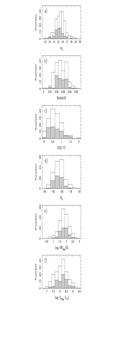
Figure 1: From top to bottom, distributions of the observed Gunn-$r$ magnitudes, redshifts, gas colour excesses, absolute Gunn-$r$ magnitudes, EW(H$\alpha$), and H$\alpha$ luminosities. The open histograms correspond to the complete UCM sample, and the grey-filled areas correspond to the nIR sample.

5.1 Sample completeness

Our nIR sample will suffer, first, from the intrinsic selection effects of the objective-prism$+$photographic plate technique used in the UCM survey. Those were discussed in detail in Zamorano et al. (1994, 1996), Vitores [Vitores 1994] and Gallego [Gallego 1995]. Briefly, the observational procedure employed limits the UCM sample to local galaxies with redshift lower than 0.045$\pm$0.005 and H$\alpha$ equivalent width larger than 20Å. The Gunn-$r$ limiting magnitude is 16.5^m with a brigth end cut-off, due to saturation of the photographic plates, placed at $\sim$14.2^m. However, additional selection effects may be present in our work due to the limited size of our nIR sample ($\sim$35 per cent of the UCM whole sample), thus it is necessary to ensure that the properties of this subsample are representative of those of the complete UCM survey.

In Figure 1a we compare the Gunn-$r$ apparent magnitude histogram of the whole UCM sample with that of the galaxies observed in the nIR. Although the apparent magnitude distributions match reasonably well, the objects in the nIR subsample tend to be marginally brighter than those in the UCM complete sample. The median $m_{r}$ for the UCM complete sample is 15.5^m, while that of the nIR sample is 15.2^m (see Vitores et al. 1996b). This may imply a small deficiency of low-luminosity and/or higher redshift galaxies. However, that does not seem to be a strong effect (see figures 1b and d).

From Figures 1b, 1c and 1e it is clear that the nIR sample represents about 35 per cent of the UCM complete sample [Gallego 1995] in every redshift, $E(B-V)$ and EW(H$\alpha$) bin. A Kolmogorov-Smirnov test indicates that both samples show similar distributions in $z$, $E(B-V)$ and EW(H$\alpha$), with probabilities of 45, 93 and 87 per cent, respectively. For the $r$-band absolute magnitudes and H$\alpha$ luminosities the probabilities are 25 and 47 per cent, respectively (see Figures 1d and 1f). Thus the galaxies in the nIR sample seem to be a fair subsample of the UCM complete sample in their global properties.

The only small difference arises when comparing in detail the spectroscopic type distributions of the star-forming galaxies in the nIR and UCM complete samples. There is a small deficiency of HII-like galaxies (see ahead) in the nIR subsample relative to the whole UCM sample. About 30 per cent of the UCM whole sample are HII-like galaxies, whereas only 19 per cent are present in the nIR subsample. Consequences of such a limitation will be taken into account in further discussions.

5.2 Aperture magnitudes and colours

5.2.1 Mean colours

Global colours (obtained inside three disk-scale lengths), together with the integrated $K$-band magnitudes (not corrected for extinction) and the $E(B-V)_{\mathrm{gas}}$ colour excesses, are given in Table LABEL:data. In GAL96, the galaxies in the UCM sample were classified in different morphological and spectroscopic classes (listed in table LABEL:data). We will briefly describe them here (see GAL96 for details):

SBN —Starburst Nuclei— Originally defined by Balzano [Balzano 1983], they show high extinction values, with very low [NII]/H$\alpha$ ratios and faint [OIII]$\lambda$5007 emission. Their H$\alpha$ luminosities are always higher than 10⁸ L_☉.

DANS —Dwarf Amorphous Nuclear Starburst— Introduced by Salzer, MacAlpine & Boroson [Salzer et al. 1989], they show very similar spectroscopic properties to SBN objects, but with H$\alpha$ luminosities lower than 5$\times$10⁷ L_☉.

HIIH —HII Hotspot— The HII Hotspot class shows (see GAL96) similar H$\alpha$ luminosities to those measured in SBN galaxies but with large [OIII]$\lambda$5007/H$\beta$ ratios, that is, higher ionization.

DHIIH —Dwarf HII Hotspot—- This is an HIIH subclass with identical spectroscopic properties but H$\alpha$ luminosities lower than 5$\times$10⁷ L_☉.

BCD —Blue Compact Dwarf— Finally, the lowest luminosity and highest ionization objects have been classified as Blue Compact Dwarf galaxies, showing in all cases H$\alpha$ luminosities lower than 5$\times$10⁷ L_☉. They also show large [OIII]$\lambda$5007/H$\beta$ and H$\alpha$/[NII]$\lambda$6584 line ratios and intense [OII]$\lambda$3727 emission.

In our analysis, we separate the galaxies in two main categories: starburst disk-like (SB hereafter) and HII-like galaxies (see Guzmán et al. 1997; Gallego 1998). The SB-like class includes SBN and DANS spectroscopic types, whereas the HII-like includes HIIH, DHIIH and BCD type galaxies.

In order to determine representative mean optical-nIR colours for each galaxy group, we have assumed Gaussian probability distributions for the $r-J$ and $J-K$ colours and EW(H$\alpha$) with the centres and widths ($\sigma$) given in Table LABEL:data. We have weighted the data for each galaxy with their corresponding errors when determining the mean values.

The HII-like objects seem to be on average 0.2^m bluer in $r-J$ and 0.1^m in $J-K$ than the SB galaxies (see Table LABEL:datamean). Since the mean colour excess of the SB population ($\overline{E(B-V)}$=0.7^m) is 0.2^m higher than that of the HII-like galaxies, these colour differences are even more significant when data not corrected for extinction are used: the differences for the un-corrected colours are 0.35^m in $r-J$ and 0.15^m in $J-K$. K-S tests performed on the SB-like and HII-like objects indicate that both subsamples arise from independent distributions with a probability of 99.7 and 99.9 per cent respectively for the un-corrected $r-J$ and $J-K$ colours.

Finally, whereas more than 60 per cent of the HII-like objects show not corrected for extinction equivalent widths of H$\alpha$ higher than 120 Å, only 3 per cent of the SB galaxies do. The relatively low EW(H$\alpha$) detection limit estimated for the UCM survey ($\sim$ 20 Å; Gallego 1995) ensures that the difference in EW(H$\alpha$) between SB and HII-like galaxies is not due to selection effects. A K-S test gives a probability of 99.9 per cent that these samples have independent EW(H$\alpha$) distributions. These differences in colours and H$\alpha$ equivalent widths are probably related to differences in their evolutionary properties (typical starburst age, starburst strength, specific star formation rate, etc) between both galaxy types (see section 5.4 and section 5.6).

5.2.2 Colour-colour and colour-EW(H$\alpha$) diagrams

In Figure 2 we show colour-colour ($r-J$ vs. $J-K$) and colour-EW(H$\alpha$) plots for the nIR sample. The offset between the position of the star forming galaxies (filled circles) in the $r-J$–$J-K$ plane (Figure 2a) and the bulges and disks of relaxed nearby spirals [Peletier & Balcells 1996] indicates the existence of ongoing star formation. Error bars in Figure 2a represent $\pm$1$\sigma$ errors. In Figures 2a and 2b we plot solar metallicity models with burst strengths, 10^-3, 10^-2, 10^-1, and 1. In the case of Figures 2c and 2d, models with 10^-1 burst strength and different metallicities are displayed (cf. section 4).

Figures 2a and 2c show that changes in the optical-nIR colours due to changes in burst strength and age are much more significant than those produced by changes in metallicity. This fact is also observed in the colour-EW(H$\alpha$) diagrams (Figures 2b and 2d), especially in the case of sub-solar metallicity models. It is thus clear that it is in principle possible to infer burst strengths and ages from these diagrams, but the determination of metallicities would be very uncertain.

Table 2: Mean colours, H$\alpha$ equivalent widths (Å), and corresponding standard deviations of the mean for the UCM nIR sample.

	n	$\overline{r-J}$  $\sigma$	$\overline{J-K}$  $\sigma$	$\overline{\mathrm{EW(H}\alpha\mathrm{)}}$  $\sigma$
Not corrected for extinction
Total	67	1.79  0.05	1.06  0.04	80  7
SB-like	49	1.88  0.05	1.10  0.05	60  5
(SBN+DANS)
HII-like (HIIH+	18	1.54  0.09	0.96  0.30	133 16
DHIIH+BCD)
Corrected for extinction
Total	66	1.26  0.05	0.87  0.06	168  10
SB-like	49	1.28  0.06	0.89  0.09	150  10
HII-like	17	1.21  0.07	0.81  0.35	220  30

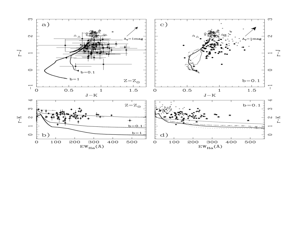
Figure 2: Colour-colour and colour-EW(H$\alpha$) diagrams. In panels a and b optical-nIR colours are plotted for the 67 galaxies of the sample. Solar metallicity models have been plotted using progresively thicker lines for higher burst strenght models ($b$=10^-3,10^-2,10^-1,1). Data for nearby relaxed spiral galaxies have been taken from Peletier & Balcells (1996); both bulge (asterisks) and disk (triangles) colours are shown. Panels c, d show the optical-nIR colours of the SB-like (dots) and the HII-like (stars) objects. Values not corrected for extinction are also shown (small circles). In panels c & d, models with 10^-1 burst strength and different metallicities from 1/50 Z_☉ to 2 Z_☉ have been drawn (1/50 Z_☉, thin solid line; 1/5 Z_☉, dashed line; 2/5 Z_☉, dashed-dotted line; Z_☉, thick solid line; 2 Z_☉, dotted line). $\pm$1$\sigma$ error bars are also shown.

5.3 Determination of the physical properties of the galaxies

For each individual galaxy we have information on its $r-J$ and $J-K$ colours and H$\alpha$ equivalent width. Thus, each galaxy has a point associated in the $r-J$, $J-K$, 2.5$\times$log EW(H$\alpha$) three-dimensional space. However, due to the calibration and photometric errors, the uncertainty in these measurements transforms these points into probability distributions. As in section 5.2.1, we will assume Gaussian probability distributions for the $r-J$, $J-K$ colours and 2.5$\times$log EW(H$\alpha$) with the centres and widths ($\sigma$) given in Table LABEL:data. The evolutionary synthesis models that we will associate with each galaxy probability distribution, will also follow different tracks in this three-dimensional space.

The three-dimensional probability distributions ($r-J$,$J-K$,2.5$\times$log EW(H$\alpha$)) have been reproduced using a Monte Carlo simulation method. A total of 10³ data points were generated in order to reproduce this distribution for each galaxy. No significant differences were observed using a larger number (e.g., 10⁴) of input particles. We estimated the model that better reproduces the colours and EW(H$\alpha$) for each of the 10³ test particles applying a maximum likelihood method. The maximum likelihood estimator used, ${\cal L}$, includes two colour terms and an EW(H$\alpha$) term. Thus,

$${\cal L}(t,b,Z)=\prod_{n=1}^{3}{1\over\sqrt{2\pi}\Delta C_{n}}\exp\left(-{(c_{n}-C_{n})^{2}\over 2\Delta C_{n}\,^{2}}\right)$$ (3)

where $C_{1}$, $C_{2}$ and $C_{3}$ are the $r-J$ and $J-K$ colours and 2.5$\times$log EW(H$\alpha$) and $\Delta C_{1}$, $\Delta C_{2}$ and $\Delta C_{3}$ are their corresponding errors. The $c_{n}$ coefficients are the $r-J$, $J-K$ and 2.5$\times$log EW(H$\alpha$) values predicted by a given model. A similar estimator was employed by Abraham et al. [Abraham et al. 1999] for a sample of intermediate-$z$ HDF [Williams et al. 1996] galaxies.

Finally, we obtained the age, $t$, burst strength, $b$, and metallicity, $Z$, of the model that maximizes ${\cal L}$ for each test particle of the ($r-J$,$J-K$,2.5$\times$log EW(H$\alpha$)) probability distribution. Therefore, this procedure effectively provides the ($t$,$b$,$Z$) probability distribution for each input galaxy.

The resulting ($t$,$b$,$Z$) probability distributions are in many cases multi-peaked. Instead of analyzing these probability distributions as a whole, we have studied the clustering pattern present in the ($t$,$b$,$Z$) solution space. We have used a single linkage hierarchical clustering method (see Murtagh & Heck 1987; see also Appendix), which allows to isolate different solutions in the ($t$,$b$,$Z$) space. We have recovered the three most representative solution clusters for each galaxy. In Table LABEL:tablafin we show the mean properties of those solution clusters with probability higher than 20 per cent. This probability is computed as the number of test particles in a given cluster over the total number of test particles (10³). The errors shown in Table LABEL:tablafin correspond to the standard deviation of the data for each solution cluster. In those cases where all the solutions within a cluster yield the same age, burst strength, metallicity or mass, no errors were given.

The subsequent statistical analysis of each of the ($t$,$b$,$Z$) clusters indicates that significant correlations between $t$, $b$ and $Z$ are present. We have performed a principal component analysis (PCA hereafter; see Morrison 1976; see also Appendix) of the individual clusters given in Table LABEL:tablafin. The orientation of the first PCA component and the contribution of this component to the total variance within the solution cluster are also given.

After applying this procedure to the observed sample, only three galaxies (UCM1440$+$2521S, UCM1506$+$1922 and UCM1513$+$2012; see Figure  3a and 3b) show ${\cal L}_{\mathrm{max}}$$<$10.0. Note that a value ${\cal L}_{\mathrm{max}}=10.0$ corresponds to a model where the differences between the observed data and the model predictions equal the measurement errors, assuming mean errors of 0.12^m in $(r-J)$ and $(J-K)$ and 10 per cent in EW(H$\alpha$). This indicates that the range of model predictions covers reasonably well the observed properties of the galaxies. In Figure 3a and 3b we plot the differences between the colours and EW(H$\alpha$) measured and those predicted by the best-fit model. These differences have been calculated for the central values of the $r-J$, $J-K$ and 2.5$\times$log EW(H$\alpha$) probability distributions.

Figure 3a shows that, in some cases, the models predict bluer $J-K$ colours than those measured. At first sight, these discrepancies could be explained if we were underestimating the extinction correction factors applied to these objects. However, since the extinction correction affects $r-J$ more than $J-K$, applying a higher extinction correction would destroy the good agreement between the observed and model $r-J$ colours. We have quantified the effect of a change in the correction for extinction assumed for our galaxies by comparing data de-reddened using $E(B-V)_{\mathrm{continuum}}$=$E(B-V)_{\mathrm{gas}}$ with our models. Figure 3c shows that data corrected using the relation given by Calzetti et al. [Calzetti et al. 1996] fit the models better than data corrected assuming $E(B-V)_{\mathrm{continuum}}$=$E(B-V)_{\mathrm{gas}}$. In addition, none of the three galaxies given above show higher ${\cal L}_{\mathrm{max}}$ values after using $E(B-V)_{\mathrm{continuum}}$=$E(B-V)_{\mathrm{gas}}$. Thus, we are confident that the extinction correction applied provides a reasonable fit to the models, and the discrepancies in $J-K$ between the data and the models are probably due to inherent uncertainties in the modelling of the nIR continuum by the Bruzual and Charlot code.

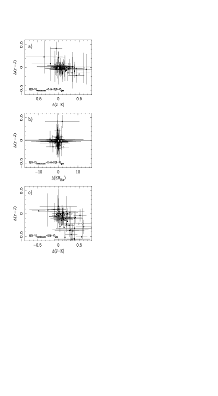
Figure 3: a) & b) Differences between the $r-J$, $J-K$ and EW(H$\alpha$) measured values and the best-fitting model values, using $E(B-V)_{\mathrm{continuum}}$=0.44$\times$$E(B-V)_{\mathrm{gas}}$. The input $r-J$, $J-K$ and EW(H$\alpha$) data correspond to the central values of the respective probability distributions. Those galaxies with ${\cal L}_{\mathrm{max}}$$<$10 are shown as grey dots. c) Differences in the $r-J$ and $J-K$ colours assuming $E(B-V)_{\mathrm{continuum}}$=$E(B-V)_{\mathrm{gas}}$.

The cluster analysis performed indicates that the clustering in the solution space is basically produced by the discretization in metallicity of the models. Fortunately, in many of the objects ($\sim$30 per cent; see Table LABEL:tablafin), only one ($t$,$b$,$Z$) solution cluster is able to reproduce the observables. About 33 per cent need two solutions and three solutions are needed for the remaining 37 per cent. The goodness of this comparison method, given by the number and size of statistically significant ($t$,$b$,$Z$) solution clusters, basically depends on the particular position of the object in the ($r-J$,$J-K$,2.5$\times$log EW(H$\alpha$)) space and on its measurement errors. Fortunately, in those cases where the ($t$,$b$,$Z$) probability distribution is multi-valuated, the different solution clusters give similar burst strengths and total stellar masses. This is another manifestation of the fact that, as we saw in section 5.2.2, our data is not very sensitive to metallicity, and we will not attempt to derive it. Nonetheless, the burst ages are affected somewhat by small changes in metallicity, and frequently show wider distributions than the burst strenghts.

Finally, the PCA performed on each solution cluster suggests that the best-axis, given by the vector ($u_{t}$,$u_{\mathrm{log}(b)}$,$u_{\mathrm{log}(Z)}$)=($u_{x}$,$u_{y}$,$u_{z}$) shown in Table LABEL:tablafin, is commonly placed in the $u_{x}$-$u_{y}$ ($t$-$b$) plane and obeys $u_{x}$$\simeq$$u_{y}$. This implies that age and burst strength are in many cases degenerated and, therefore, the properties of an individual object can be reproduced both with a young, low burst strength or an old, high burst strength model, within the ranges given in Table LABEL:tablafin.

Table 3: Best fit model results for the nIR sample.

Galaxy	Prob.	Age	log $b$	log ($Z/Z_{\sun}$)	log ($M/M_{\sun})$	PCA	Variance
	(%)	(Myr)	($b$=$M_{\mathrm{young}}$/$M_{\mathrm{total}}$)			($u_{t}$,$u_{\mathrm{log}\,b}$,$u_{\mathrm{log}\,Z}$)	(%)
0003$+$2200	39.1	6.91$\pm$0.56	$-$0.981$\pm$0.410	$-$0.60$\pm$0.14	10.18$\pm$0.21(0.14)	($+$0.666,$+$0.477,$-$0.574)	73.7
	36.7	11.55$\pm$0.48	$-$0.813$\pm$0.277	$-$1.70	10.44$\pm$0.05(0.14)	($+$0.707,$+$0.707,$+$0.000)	62.1
	24.2	4.55$\pm$0.68	$-$1.519$\pm$0.380	$+$0.31$\pm$0.16	10.31$\pm$0.27(0.14)	($+$0.679,$+$0.528,$-$0.510)	70.0
0013$+$1942	43.2	4.85$\pm$0.67	$-$1.846$\pm$0.128	$-$0.30$\pm$0.32	10.10$\pm$0.01(0.03)	($+$0.634,$+$0.523,$-$0.569)	82.1
	33.5	8.86$\pm$0.37	$-$1.436$\pm$0.103	$-$1.70	10.12        (0.03)	($+$0.707,$+$0.707,$+$0.000)	65.7
	23.3	3.18$\pm$0.10	$-$1.959$\pm$0.093	$+$0.40	10.11$\pm$0.01(0.03)	($+$0.707,$+$0.707,$+$0.000)	63.0
0014$+$1748	62.8	4.33$\pm$0.71	$-$2.024$\pm$0.192	$-$0.59$\pm$0.21	11.00$\pm$0.01(0.02)	($+$0.708,$+$0.630,$-$0.319)	64.7
	28.4	4.93$\pm$1.43	$-$2.101$\pm$0.286	$-$1.70	11.00$\pm$0.01(0.02)	($+$0.707,$+$0.707,$+$0.000)	66.5
0014$+$1829	36.8	3.31$\pm$0.28	$-$1.194$\pm$0.188	$-$0.40$\pm$0.32	10.09$\pm$0.08(0.08)	($+$0.710,$+$0.439,$-$0.550)	62.6
	32.2	1.73$\pm$0.30	$-$1.131$\pm$0.207	$+$0.40	10.11$\pm$0.07(0.08)	($+$0.707,$+$0.707,$+$0.000)	58.5
	31.0	3.81$\pm$0.66	$-$0.885$\pm$0.464	$-$1.70	9.87$\pm$0.28(0.08)	($+$0.707,$+$0.707,$+$0.000)	56.9
0015$+$2212	53.2	3.41$\pm$0.81	$-$2.159$\pm$0.170	$+$0.23$\pm$0.20	10.20$\pm$0.01(0.03)	($+$0.621,$+$0.561,$-$0.547)	84.1
	24.3	4.77$\pm$0.70	$-$2.135$\pm$0.274	$-$0.60$\pm$0.14	10.19$\pm$0.01(0.03)	($+$0.623,$+$0.676,$+$0.394)	71.3
	22.5	7.71$\pm$1.54	$-$1.796$\pm$0.318	$-$1.70	10.20        (0.03)	($+$0.707,$+$0.707,$+$0.000)	66.5
0017$+$1942	67.9	4.80$\pm$0.61	$-$1.613$\pm$0.187	$-$0.42$\pm$0.31	10.51$\pm$0.02(0.03)	($+$0.719,$+$0.436,$-$0.541)	63.6
	20.6	8.32$\pm$0.47	$-$1.256$\pm$0.144	$-$1.70	10.53$\pm$0.01(0.03)	($+$0.707,$+$0.707,$+$0.000)	65.3
0022$+$2049	42.6	1.93$\pm$0.67	$-$2.214$\pm$0.147	$+$0.40	10.98        (0.02)	($+$0.707,$+$0.707,$+$0.000)	63.0
	34.6	3.32$\pm$1.03	$-$2.215$\pm$0.249	$-$0.30$\pm$0.29	10.98$\pm$0.01(0.02)	($+$0.717,$+$0.661,$-$0.224)	61.8
	22.8	5.22$\pm$1.80	$-$2.014$\pm$0.327	$-$1.70	10.98$\pm$0.01(0.02)	($+$0.707,$+$0.707,$+$0.000)	66.3
0050$+$2114	52.2	4.76$\pm$0.71	$-$1.889$\pm$0.224	$-$0.48$\pm$0.28	11.03$\pm$0.01(0.04)	($+$0.706,$+$0.569,$-$0.421)	65.9
	27.0	2.75$\pm$0.37	$-$2.081$\pm$0.109	$+$0.40	11.04$\pm$0.01(0.04)	($+$0.707,$+$0.707,$+$0.000)	61.3
	20.8	7.58$\pm$1.26	$-$1.643$\pm$0.273	$-$1.70	11.04        (0.04)	($+$0.707,$+$0.707,$+$0.000)	66.3
0145$+$2519	72.1	11.56$\pm$0.17	$-$0.979$\pm$0.107	$-$1.70	11.30$\pm$0.02(0.04)	($+$0.707,$+$0.707,$+$0.000)	64.5
1255$+$3125	63.7	4.78$\pm$0.99	$-$1.423$\pm$0.650	$+$0.34$\pm$0.14	10.28$\pm$0.45(0.07)	($+$0.618,$+$0.683,$+$0.389)	67.9
	22.3	5.13$\pm$1.36	$-$2.144$\pm$0.397	$-$0.55$\pm$0.15	10.71$\pm$0.04(0.07)	($+$0.688,$+$0.702,$+$0.182)	65.2
1256$+$2823	66.5	3.65$\pm$0.45	$-$1.701$\pm$0.100	$+$0.35$\pm$0.13	10.88$\pm$0.01(0.04)	($+$0.683,$+$0.369,$-$0.631)	70.8
	28.0	9.84$\pm$0.43	$-$1.162$\pm$0.140	$-$1.70	10.89$\pm$0.01(0.04)	($+$0.707,$+$0.707,$+$0.000)	66.3
1257$+$2808	59.6	11.46$\pm$0.18	$-$0.405$\pm$0.148	$-$1.70	10.22$\pm$0.03(0.11)	($+$0.707,$+$0.707,$+$0.000)	64.2
	38.5	4.47$\pm$0.54	$-$1.138$\pm$0.249	$+$0.32$\pm$0.16	10.10$\pm$0.19(0.11)	($+$0.650,$+$0.484,$-$0.586)	77.9
1259$+$2755	85.1	4.35$\pm$0.50	$-$1.234$\pm$0.240	$+$0.34$\pm$0.14	10.71$\pm$0.17(0.05)	($+$0.658,$+$0.488,$-$0.574)	76.4
1259$+$3011	84.1	13.84$\pm$0.32	$-$0.923$\pm$0.146	$-$1.70	10.79$\pm$0.03(0.06)	($+$0.707,$+$0.707,$+$0.000)	65.7
1302$+$2853	57.7	6.98$\pm$0.55	$-$1.471$\pm$0.271	$-$0.60$\pm$0.14	10.40$\pm$0.12(0.08)	($+$0.700,$+$0.380,$-$0.605)	66.4
	25.4	11.65$\pm$0.36	$-$1.154$\pm$0.148	$-$1.70	10.51$\pm$0.01(0.08)	($+$0.707,$+$0.707,$+$0.000)	65.7
1304$+$2808	82.6	13.96$\pm$0.96	$-$1.487$\pm$0.216	$-$1.70	10.71$\pm$0.01(0.06)	($+$0.707,$+$0.707,$+$0.000)	66.3
1304$+$2818	89.0	3.47$\pm$0.28	$-$1.988$\pm$0.143	$+$0.39$\pm$0.06	10.68$\pm$0.01(0.04)	($+$0.720,$+$0.656,$-$0.225)	61.1
1306$+$2938	66.8	3.37$\pm$0.22	$-$1.746$\pm$0.096	$+$0.39$\pm$0.07	10.67$\pm$0.01(0.04)	($+$0.711,$+$0.309,$-$0.632)	65.4
	32.0	9.31$\pm$0.27	$-$1.248$\pm$0.087	$-$1.70	10.68        (0.04)	($+$0.707,$+$0.707,$+$0.000)	65.0
1307$+$2910	46.4	12.38$\pm$0.77	$-$0.884$\pm$0.317	$-$1.70	11.25$\pm$0.07(0.11)	($+$0.707,$+$0.707,$+$0.000)	61.5
	46.3	6.97$\pm$1.07	$-$1.157$\pm$0.537	$-$0.44$\pm$0.29	11.02$\pm$0.26(0.11)	($+$0.690,$+$0.387,$-$0.612)	66.7
1308$+$2950	39.7	5.21$\pm$0.59	$-$1.559$\pm$0.131	$-$0.38$\pm$0.30	11.40$\pm$0.02(0.04)	($+$0.631,$+$0.505,$-$0.589)	82.0
	35.2	9.19$\pm$0.27	$-$1.170$\pm$0.094	$-$1.70	11.43        (0.04)	($+$0.707,$+$0.707,$+$0.000)	65.9
	25.1	3.25$\pm$0.08	$-$1.695$\pm$0.099	$+$0.40	11.41$\pm$0.01(0.04)	($+$0.707,$+$0.707,$+$0.000)	65.6
1308$+$2958	37.0	7.60$\pm$0.06	$-$0.738$\pm$0.146	$-$0.70	10.47$\pm$0.11(0.06)	($+$0.707,$+$0.707,$+$0.000)	61.6
	35.7	5.75	$-$0.717$\pm$0.101	$+$0.00	10.38$\pm$0.07(0.06)	($+$0.000,$+$1.000,$+$0.000)	100.0
	27.3	12.00	$-$0.647$\pm$0.038	$-$1.70	10.76$\pm$0.01(0.06)	($+$0.000,$+$1.000,$+$0.000)	100.0
1312$+$2954	39.8	5.89$\pm$0.28	$-$1.438$\pm$0.208	$-$0.54$\pm$0.15	10.71$\pm$0.09(0.13)	($+$0.743,$+$0.207,$-$0.636)	56.5
	39.2	3.79$\pm$0.55	$-$1.642$\pm$0.172	$+$0.33$\pm$0.15	10.76$\pm$0.05(0.13)	($+$0.675,$+$0.408,$-$0.615)	71.9
	21.0	9.99$\pm$0.56	$-$1.114$\pm$0.171	$-$1.70	10.79$\pm$0.01(0.13)	($+$0.707,$+$0.707,$+$0.000)	64.8
1312$+$3040	73.4	3.69$\pm$0.39	$-$2.073$\pm$0.181	$+$0.37$\pm$0.10	10.86$\pm$0.05(0.03)	($+$0.739,$+$0.540,$-$0.403)	60.5
	25.2	9.87$\pm$0.63	$-$1.577$\pm$0.144	$-$1.70	10.88        (0.03)	($+$0.707,$+$0.707,$+$0.000)	66.4
1428$+$2727	53.1	3.49$\pm$0.13	$-$1.400$\pm$0.145	$+$0.40	10.17$\pm$0.03(0.07)	($+$0.707,$+$0.707,$+$0.000)	65.4
	25.6	9.97$\pm$0.41	$-$0.809$\pm$0.209	$-$1.70	10.20$\pm$0.03(0.07)	($+$0.707,$+$0.707,$+$0.000)	66.1
	21.3	5.53$\pm$0.49	$-$1.146$\pm$0.268	$-$0.37$\pm$0.26	10.07$\pm$0.12(0.07)	($+$0.663,$+$0.447,$-$0.600)	74.6
1432$+$2645	65.6	11.49$\pm$0.07	$-$0.974$\pm$0.042	$-$1.70	11.14        (0.04)	($+$0.707,$+$0.707,$+$0.000)	60.8
	25.9	4.50$\pm$0.52	$-$1.610$\pm$0.079	$+$0.32$\pm$0.16	11.08$\pm$0.03(0.04)	($+$0.617,$+$0.527,$-$0.585)	86.0
1440$+$2511	96.7	12.60$\pm$0.03	$-$0.882$\pm$0.030	$-$1.70	10.78        (0.05)	($+$0.707,$+$0.707,$-$0.004)	47.9
1440$+$2521N	42.8	3.58$\pm$0.74	$-$1.724$\pm$0.502	$+$0.40	10.80$\pm$0.25(0.12)	($+$0.707,$+$0.707,$+$0.000)	64.6
	33.2	4.95$\pm$1.20	$-$1.871$\pm$0.458	$-$0.33$\pm$0.29	10.86$\pm$0.08(0.12)	($+$0.704,$+$0.664,$-$0.250)	64.6
	24.0	8.09$\pm$3.17	$-$1.660$\pm$0.661	$-$1.70	10.90$\pm$0.03(0.12)	($+$0.707,$+$0.707,$+$0.000)	65.8
1440$+$2521S	61.6	3.88$\pm$0.66	$-$1.788$\pm$0.352	$+$0.36$\pm$0.11	10.52$\pm$0.15(0.12)	($+$0.720,$+$0.671,$-$0.178)	62.2
	31.8	9.89$\pm$2.78	$-$1.295$\pm$0.621	$-$1.70	10.57$\pm$0.03(0.12)	($+$0.707,$+$0.707,$+$0.000)	65.6
1442$+$2845	59.0	4.55$\pm$0.63	$-$1.986$\pm$0.193	$-$0.41$\pm$0.31	10.32$\pm$0.01(0.04)	($+$0.738,$+$0.532,$-$0.415)	60.6
	20.6	7.47$\pm$1.42	$-$1.705$\pm$0.302	$-$1.70	10.32        (0.04)	($+$0.707,$+$0.707,$+$0.000)	66.4
	20.4	2.70$\pm$0.42	$-$2.149$\pm$0.130	$+$0.40	10.32$\pm$0.01(0.04)	($+$0.707,$+$0.707,$+$0.000)	63.2

Table 3: (cont.) Best fit model results for the nIR sample.

Galaxy	Prob.	Age	log $b$	log ($Z/Z_{\sun}$)	log ($M/M_{\sun}$)	PCA	Variance
	(%)	(Myr)	($b$=$M_{\mathrm{young}}$/$M_{\mathrm{total}}$)			($u_{t}$,$u_{\mathrm{log}\,b}$,$u_{\mathrm{log}\,Z}$)	(%)
1443$+$2548	62.3	5.00$\pm$1.47	$-$1.767$\pm$0.572	$-$0.40$\pm$0.26	10.89$\pm$0.10(0.10)	($+$0.702,$+$0.710,$+$0.061)	62.4
	24.0	4.89$\pm$3.56	$-$2.275$\pm$0.706	$-$1.70	10.98$\pm$0.03(0.10)	($+$0.707,$+$0.707,$+$0.000)	65.7
1452$+$2754	52.3	3.13$\pm$1.39	$-$2.398$\pm$0.462	$-$0.57$\pm$0.24	11.13$\pm$0.04(0.10)	($+$0.673,$+$0.704,$+$0.226)	65.8
	37.8	2.52$\pm$2.14	$-$2.573$\pm$0.367	$-$1.70	11.14$\pm$0.01(0.10)	($+$0.707,$+$0.707,$+$0.000)	65.5
1506$+$1922	46.6	2.81$\pm$2.98	$-$2.690$\pm$0.518	$-$1.70	10.82$\pm$0.01(0.10)	($+$0.707,$+$0.707,$+$0.000)	66.1
	33.1	4.05$\pm$1.68	$-$2.252$\pm$0.559	$-$0.44$\pm$0.29	10.78$\pm$0.10(0.10)	($+$0.698,$+$0.708,$+$0.107)	63.4
	20.3	3.55$\pm$1.36	$-$1.675$\pm$0.894	$+$0.40	10.46$\pm$0.56(0.10)	($+$0.707,$+$0.707,$+$0.000)	64.6
1513$+$2012	90.3	2.75$\pm$0.59	$-$2.137$\pm$0.117	$+$0.31$\pm$0.17	11.29        (0.03)	($+$0.644,$+$0.508,$-$0.572)	76.5
1557$+$1423	42.5	11.71$\pm$0.41	$-$1.450$\pm$0.118	$-$1.70	10.61$\pm$0.01(0.02)	($+$0.707,$+$0.707,$+$0.000)	66.2
	34.6	4.39$\pm$0.56	$-$2.167$\pm$0.162	$+$0.32$\pm$0.16	10.59$\pm$0.03(0.02)	($+$0.695,$+$0.499,$-$0.518)	67.9
	22.9	7.16$\pm$0.54	$-$1.824$\pm$0.165	$-$0.64$\pm$0.12	10.57$\pm$0.03(0.02)	($+$0.651,$+$0.530,$-$0.544)	77.8
1646$+$2725	35.2	2.89$\pm$1.43	$-$2.231$\pm$0.329	$-$0.60$\pm$0.14	9.93$\pm$0.02(0.05)	($+$0.688,$+$0.693,$+$0.214)	64.3
	34.2	3.00$\pm$2.20	$-$2.248$\pm$0.365	$-$1.70	9.93$\pm$0.01(0.05)	($+$0.707,$+$0.707,$+$0.000)	66.3
	30.6	1.78$\pm$0.91	$-$2.179$\pm$0.187	$+$0.28$\pm$0.18	9.94$\pm$0.01(0.05)	($+$0.720,$+$0.681,$-$0.133)	59.1
1647$+$2729	66.4	4.66$\pm$0.59	$-$1.090$\pm$0.668	$+$0.31$\pm$0.17	10.53$\pm$0.51(0.02)	($+$0.514,$+$0.764,$+$0.390)	56.6
1647$+$2950	38.2	4.87$\pm$1.29	$-$1.769$\pm$0.515	$-$0.57$\pm$0.15	11.02$\pm$0.08(0.11)	($+$0.635,$+$0.679,$+$0.369)	68.1
	36.6	3.45$\pm$1.05	$-$1.881$\pm$0.385	$+$0.19$\pm$0.20	11.05$\pm$0.06(0.11)	($+$0.688,$+$0.584,$-$0.431)	66.5
	25.2	6.21$\pm$3.25	$-$1.848$\pm$0.663	$-$1.70	11.08$\pm$0.01(0.11)	($+$0.707,$+$0.707,$+$0.000)	66.2
1648$+$2855	92.2	2.71$\pm$0.47	$-$1.777$\pm$0.085	$+$0.35$\pm$0.14	10.78$\pm$0.01(0.05)	($+$0.623,$+$0.518,$-$0.586)	78.7
1654$+$2812	60.9	4.30$\pm$0.62	$-$1.756$\pm$0.242	$+$0.34$\pm$0.14	9.92$\pm$0.14(0.07)	($+$0.697,$+$0.528,$-$0.486)	67.8
	20.2	6.43$\pm$0.47	$-$1.577$\pm$0.211	$-$0.53$\pm$0.15	9.91$\pm$0.07(0.07)	($+$0.692,$+$0.447,$-$0.567)	68.1
1656$+$2744	55.6	4.45$\pm$1.13	$-$2.164$\pm$0.295	$-$0.30$\pm$0.26	10.72$\pm$0.01(0.04)	($+$0.666,$+$0.628,$-$0.403)	71.4
	22.2	8.15$\pm$1.33	$-$1.773$\pm$0.283	$-$1.70	10.72        (0.04)	($+$0.707,$+$0.707,$+$0.000)	66.3
	22.2	2.82$\pm$0.94	$-$2.174$\pm$0.389	$+$0.40	10.70$\pm$0.14(0.04)	($+$0.707,$+$0.707,$+$0.000)	63.4
1657$+$2901	84.3	3.94$\pm$0.40	$-$1.760$\pm$0.190	$+$0.38$\pm$0.09	10.52$\pm$0.07(0.05)	($+$0.703,$+$0.526,$-$0.479)	67.3
2238$+$2308	63.8	5.67$\pm$0.21	$-$1.593$\pm$0.106	$-$0.65$\pm$0.11	11.22$\pm$0.02(0.02)	($+$0.749,$+$0.169,$-$0.640)	54.6
	23.7	3.89$\pm$0.73	$-$1.664$\pm$0.142	$+$0.23$\pm$0.20	11.22$\pm$0.01(0.02)	($+$0.615,$+$0.527,$-$0.586)	86.2
2239$+$1959	68.8	3.19$\pm$0.65	$-$1.895$\pm$0.130	$+$0.25$\pm$0.19	11.11$\pm$0.01(0.02)	($+$0.606,$+$0.556,$-$0.569)	88.3
2250$+$2427	87.4	2.27$\pm$0.66	$-$2.056$\pm$0.131	$+$0.32$\pm$0.16	11.49$\pm$0.01(0.02)	($+$0.714,$+$0.466,$-$0.523)	63.2
2251$+$2352	51.5	4.27$\pm$0.40	$-$1.943$\pm$0.113	$+$0.38$\pm$0.09	10.39$\pm$0.04(0.02)	($+$0.683,$+$0.533,$-$0.499)	70.9
	35.4	11.40$\pm$0.48	$-$1.304$\pm$0.139	$-$1.70	10.43$\pm$0.01(0.02)	($+$0.707,$+$0.707,$+$0.000)	66.2
2253$+$2219	48.0	4.65$\pm$0.69	$-$2.152$\pm$0.149	$-$0.21$\pm$0.30	10.72$\pm$0.01(0.02)	($+$0.643,$+$0.536,$-$0.546)	80.3
	31.3	8.49$\pm$0.73	$-$1.794$\pm$0.167	$-$1.70	10.72        (0.02)	($+$0.707,$+$0.707,$+$0.000)	66.6
	20.7	3.46$\pm$0.95	$-$1.945$\pm$0.757	$+$0.40	10.50$\pm$0.51(0.02)	($+$0.707,$+$0.707,$+$0.000)	65.6
2255$+$1654	63.0	3.79$\pm$0.67	$-$1.963$\pm$0.116	$+$0.21$\pm$0.20	11.51$\pm$0.01(0.02)	($+$0.649,$+$0.475,$-$0.594)	77.6
	30.3	9.26$\pm$0.22	$-$1.401$\pm$0.062	$-$1.70	11.52        (0.02)	($+$0.707,$+$0.707,$+$0.000)	66.6
2255$+$1926	73.2	13.08$\pm$0.34	$-$1.135$\pm$0.133	$-$1.70	10.02$\pm$0.01(0.03)	($+$0.707,$+$0.707,$+$0.000)	65.9
2255$+$1930N	65.5	3.53$\pm$0.74	$-$2.102$\pm$0.152	$+$0.18$\pm$0.20	10.86$\pm$0.01(0.02)	($+$0.643,$+$0.530,$-$0.552)	79.6
	20.1	5.02$\pm$0.55	$-$2.014$\pm$0.225	$-$0.54$\pm$0.15	10.85$\pm$0.01(0.02)	($+$0.679,$+$0.709,$+$0.192)	65.5
2255$+$1930S	49.9	4.15$\pm$0.39	$-$1.955$\pm$0.149	$+$0.40	10.38$\pm$0.06(0.02)	($+$0.707,$+$0.707,$+$0.000)	66.0
	28.7	6.15$\pm$0.73	$-$1.853$\pm$0.196	$-$0.42$\pm$0.30	10.39$\pm$0.03(0.02)	($+$0.661,$+$0.500,$-$0.559)	75.8
	21.4	10.97$\pm$0.57	$-$1.428$\pm$0.154	$-$1.70	10.42$\pm$0.01(0.02)	($+$0.707,$+$0.707,$+$0.000)	66.4
2258$+$1920	67.8	1.32$\pm$0.92	$-$2.692$\pm$0.102	$-$1.70	10.65        (0.02)	($+$0.707,$+$0.707,$+$0.000)	61.1
	24.0	1.52$\pm$1.12	$-$2.576$\pm$0.115	$-$0.36$\pm$0.25	10.65        (0.02)	($+$0.643,$+$0.708,$+$0.293)	60.6
2300$+$2015	77.3	1.27$\pm$0.58	$-$2.713$\pm$0.062	$-$1.70	10.90        (0.02)	($+$0.707,$+$0.707,$+$0.000)	56.5
2302$+$2053E	79.5	4.34$\pm$0.47	$-$1.349$\pm$0.123	$+$0.35$\pm$0.14	11.23$\pm$0.06(0.02)	($+$0.613,$+$0.532,$-$0.584)	86.7
2302$+$2053W	49.4	2.38$\pm$0.95	$-$2.239$\pm$0.142	$-$0.38$\pm$0.27	10.23$\pm$0.01(0.03)	($+$0.734,$+$0.605,$-$0.308)	57.8
	26.3	1.26$\pm$0.63	$-$2.117$\pm$0.096	$+$0.40	10.23        (0.03)	($+$0.707,$+$0.707,$+$0.000)	58.3
	24.3	3.65$\pm$1.20	$-$2.077$\pm$0.253	$-$1.70	10.21$\pm$0.01(0.03)	($+$0.707,$+$0.707,$+$0.000)	65.2
2303$+$1856	55.5	3.47$\pm$0.72	$-$1.856$\pm$0.164	$+$0.19$\pm$0.20	11.27$\pm$0.01(0.02)	($+$0.608,$+$0.554,$-$0.569)	88.7
	23.1	8.40$\pm$0.55	$-$1.334$\pm$0.155	$-$1.70	11.28        (0.02)	($+$0.707,$+$0.707,$+$0.000)	66.1
	21.4	5.09$\pm$0.40	$-$1.721$\pm$0.170	$-$0.55$\pm$0.15	11.26$\pm$0.01(0.02)	($+$0.710,$+$0.691,$-$0.136)	64.9
2304$+$1640	47.6	4.97$\pm$0.65	$-$1.587$\pm$0.186	$-$0.33$\pm$0.31	9.43$\pm$0.03(0.06)	($+$0.647,$+$0.502,$-$0.574)	78.5
	31.7	8.90$\pm$0.51	$-$1.198$\pm$0.175	$-$1.70	9.45$\pm$0.01(0.06)	($+$0.707,$+$0.707,$+$0.000)	66.1
	20.7	3.17$\pm$0.17	$-$1.710$\pm$0.153	$+$0.40	9.44$\pm$0.02(0.06)	($+$0.707,$+$0.707,$+$0.000)	62.3
2307$+$1947	50.0	4.21$\pm$1.50	$-$2.355$\pm$0.516	$+$0.28$\pm$0.18	10.73$\pm$0.18(0.03)	($+$0.680,$+$0.704,$+$0.204)	65.7
	33.2	8.59$\pm$4.48	$-$2.173$\pm$0.802	$-$1.70	10.81$\pm$0.01(0.03)	($+$0.707,$+$0.707,$+$0.000)	66.5
2310$+$1800	45.2	4.46$\pm$1.14	$-$2.230$\pm$0.271	$-$0.34$\pm$0.29	11.15$\pm$0.01(0.03)	($+$0.714,$+$0.673,$-$0.193)	63.2
	28.2	3.10$\pm$1.22	$-$2.072$\pm$0.678	$+$0.40	10.99$\pm$0.36(0.03)	($+$0.707,$+$0.707,$+$0.000)	64.4
	26.6	6.98$\pm$2.85	$-$2.032$\pm$0.520	$-$1.70	11.15        (0.03)	($+$0.707,$+$0.707,$+$0.000)	66.4
2313$+$1841	70.2	5.03$\pm$0.65	$-$1.777$\pm$0.184	$-$0.43$\pm$0.29	10.65$\pm$0.02(0.04)	($+$0.675,$+$0.510,$-$0.534)	72.5
2316$+$2028	99.8	0.92$\pm$0.36	$-$2.731$\pm$0.026	$-$1.70	10.65        (0.04)	($+$0.707,$+$0.707,$+$0.002)	39.0
2316$+$2457	43.0	4.69$\pm$0.65	$-$2.069$\pm$0.233	$-$0.62$\pm$0.13	11.63$\pm$0.01(0.04)	($+$0.703,$+$0.709,$+$0.059)	65.1

Table 3: (cont.) Best fit model results for the nIR sample.

Galaxy	Prob.	Age	log $b$	log ($Z/Z_{\sun}$)	log ($M/M_{\sun}$)	PCA	Variance
	(%)	(Myr)	($b$=$M_{\mathrm{young}}$/$M_{\mathrm{total}}$)			($u_{t}$,$u_{\mathrm{log}\,b}$,$u_{\mathrm{log}\,Z}$)	(%)
2316$+$2457	35.5	2.96$\pm$0.89	$-$2.167$\pm$0.232	$+$0.24$\pm$0.20	11.63$\pm$0.01(0.04)	($+$0.679,$+$0.599,$-$0.424)	68.9
	21.5	6.60$\pm$1.81	$-$1.907$\pm$0.343	$-$1.70	11.64        (0.04)	($+$0.707,$+$0.707,$+$0.000)	66.4
2316$+$2459	71.6	4.90$\pm$1.28	$-$1.256$\pm$0.794	$+$0.36$\pm$0.12	10.37$\pm$0.50(0.04)	($+$0.616,$+$0.652,$+$0.443)	73.4
2319$+$2234	81.1	1.37$\pm$0.37	$-$2.838$\pm$0.030	$-$1.70	10.85        (0.04)	($+$0.707,$+$0.707,$+$0.000)	52.0
2321$+$2149	61.0	4.51$\pm$0.57	$-$1.617$\pm$0.219	$+$0.33$\pm$0.15	10.62$\pm$0.15(0.04)	($+$0.715,$+$0.488,$-$0.500)	64.7
	30.6	6.40$\pm$0.36	$-$1.553$\pm$0.226	$-$0.56$\pm$0.15	10.65$\pm$0.09(0.04)	($+$0.733,$+$0.152,$-$0.663)	57.7
2324$+$2448	57.3	6.96$\pm$2.30	$-$1.717$\pm$1.105	$+$0.33$\pm$0.16	10.77$\pm$0.43(0.04)	($+$0.648,$+$0.692,$+$0.317)	67.3
	25.0	13.51$\pm$2.61	$-$2.229$\pm$0.446	$-$1.70	11.24        (0.04)	($+$0.707,$+$0.707,$+$0.000)	66.3
2327$+$2515N	35.7	5.89$\pm$0.99	$-$1.391$\pm$0.209	$-$1.70	10.25$\pm$0.01(0.07)	($+$0.707,$+$0.707,$+$0.000)	66.1
	33.1	2.28$\pm$0.30	$-$1.602$\pm$0.125	$+$0.40	10.24$\pm$0.01(0.07)	($+$0.707,$+$0.707,$+$0.000)	60.6
	31.2	3.94$\pm$0.43	$-$1.548$\pm$0.179	$-$0.42$\pm$0.29	10.22$\pm$0.02(0.07)	($+$0.741,$+$0.473,$-$0.476)	58.6
2327$+$2515S	81.9	4.25$\pm$0.46	$-$1.253$\pm$0.370	0.37$\pm$0.11	10.15$\pm$0.29(0.06)	($+$0.711,$+$0.494,$-$0.501)	65.5

Table 4: Mean properties and standard deviations for the nIR sample. Dwarfs includes the DHIIH and BCD spectroscopic type galaxies.

	n	$\overline{t}$   $\sigma$	$\!\!\!\overline{\mathrm{log}b}$    $\sigma$	$\!\!\!\overline{\mathrm{log}Z}$  $\sigma$	$\!\!\!\!\!\!\overline{\mathrm{log}M}$    $\!\sigma$
		(Myr)
with $E(B-V)_{\mathrm{continuum}}$=0.44$\times$$E(B-V)_{\mathrm{gas}}$
Total	67	5.5  0.4	$-$1.72   0.07	$-$0.5   0.1	10.69   0.06
SBN	41	5.8   0.5	$-$1.69   0.10	$-$0.5   0.1	10.90   0.06
DANS	8	5.7   1.6	$-$1.91   0.23	$-$0.8   0.3	10.57   0.06
HIIH	13	4.1   0.6	$-$1.72   0.15	$-$0.3   0.2	10.42   0.10
Dwarfs	5	6.6   1.7	$-$1.62   0.20	$-$0.7   0.4	9.93   0.15
SB	49	5.8   0.5	$-$1.73   0.09	$-$0.6   0.1	10.85   0.05
HII	18	4.7   0.7	$-$1.69   0.10	$-$0.4   0.2	10.29   0.10
with $E(B-V)_{\mathrm{continuum}}=E(B-V)_{\mathrm{gas}}$
Total	67	11.5  0.6	$-$0.77   0.07	$-$1.2   0.1	10.64   0.05
SB	49	12.5  0.6	$-$0.69   0.08	$-$1.4   0.1	10.77   0.05
HII	18	8.3  1.0	$-$1.01   0.11	$-$0.7   0.2	10.26   0.11

5.4 Burst strengths and ages

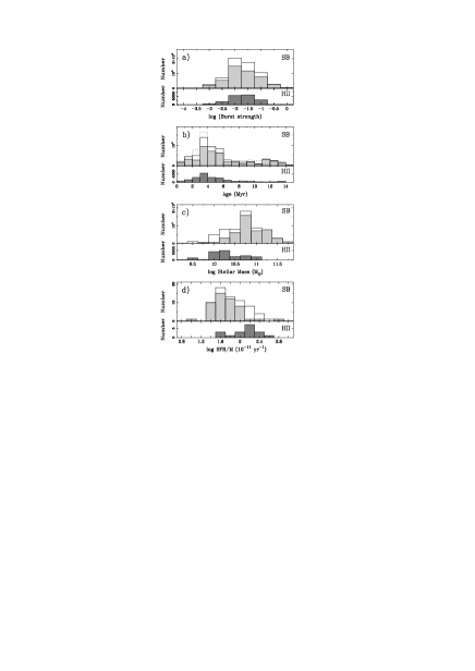
Figure 4: Frequency histograms of the derived physical properties; a) Burst strength, b) age, c) $K$-band stellar mass, and d) specific SFR (SFR per unit mass). Upper panels show the histograms for the whole sample (open histograms) and for the SB-like objects (light-grey filled histograms). Lower-panels are the frequency histograms of the HII-like galaxies (dark-grey filled histograms).

In Table LABEL:tablafin we give mean burst strengths and ages for the individual solutions with probability higher than 20 per cent. Errors given are the standard deviations of the data points in each solution. For the stellar masses, the error related with the uncertainty in the $K$-band absolute magnitude determination is also given (in parenthesis). Using these probability distributions we have derived the burst strength, age, mass and metallicity frequency histograms for the whole sample as well as for the SB-like and HII-like galaxies (see Figures 4a–d). The number of points in the $y$ axis of these figures corresponds to the number of Monte Carlo test particles with a given burst strength, age, mass or metallicity within the accepted high-probability solutions.

This analysis yields a typical burst strength of 2$\times$10^-2 with approximately 90 per cent of the sample having burst strengths between 10^-3 and 10^-1. Only seven objects in the sample show burst strengths higher than 10^-1 with a probability larger than 50 per cent, UCM0003$+$2200, UCM0145$+$2519, UCM1257$+$2808, UCM1259$+$3011, UCM1308$+$2958, UCM1432$+$2645 and UCM1440$+$2511.

Although the properties of the local star-forming galaxies seem to be well reproduced with an episodic star formation history (see also AH96), some of these objects may have evolved under more constant star formation rates (Glazebrook et al. 1999; Coziol 1996). In those objects the instantaneous burst assumption could yield very high burst strengths.

The burst strength histograms shown in Figure 4a give typically larger burst strengths for the HII-like objects, especially for the DHIIH and BCD type galaxies, than for the SB-like (see also Table LABEL:resmean). This segregation in burst strength is probably related to the difference in mean EW(H$\alpha$) pointed out in section 5.2.1 (see Table LABEL:datamean). In Table LABEL:resmean we also show the burst strengths and ages derived under the unrealistic assumption that the continuum extinction is as high as that measured for the ionized gas (see section 5.3).

The distribution of the burst ages is shown in Figure 4b. Since the probability of detection increases with EW(H$\alpha$) in objective-prism surveys (see García-Dabó et al. 1999), and the EW(H$\alpha$) continuously decreases with the the burst age, the number of objects detected with old burst ages is expected to be lower than with young ages, as observed. This behaviour is observed at ages older than 4 Myr, both for the SB and HII-like galaxies.

However, one would expect a reasonably flat distribution in the number of objects with young ages if the sample selection depended only on the H$\alpha$ equivalent width. But other factors such as the H$\alpha$ flux and continuum luminosity play an important role (see García-Dabó et al. 1999). Moreover, in our models we have estimated the H$\alpha$ luminosity ($L_{\mathrm{H}\alpha}$) from the number of Lyman continuum photons (Brocklehurst 1971) assuming that no ionizing photons escape from the galaxies. If some Lyman photons escape, the predicted H$\alpha$ luminosity would be lower and the derived ages could be significantly younger. Recent studies estimate the fraction of Lyman photons escaping from starburst galaxies to be about 3 per cent [Leitherer et al. 1995]. Bland-Hawthorn & Maloney [Bland-Hawthorn & Maloney 1997] estimated this quantity to be about 5 per cent for the Milky Way. Another feasible explanation could be that a significant fraction of these Lyman photons is absorbed by dust within the ionized gas (see, e.g., Armand et al. 1996). Both mechanisms would produce lower H$\alpha$ equivalent widths than those predicted by the standard super-ionizing models, and could explain the paucity of young star-forming bursts in Figure 4b. In this figure (dotted line) we also show the age distribution obtained assuming that 25 per cent of the Lyman continuum photons are missing. This distribution yields a larger number of objects at ages younger than 3 Myr, and a very steep decay at ages older than 4–5 Myr.

Finally, Bernasconi & Maeder [Bernasconi & Maeder 1996] have argued that, during the first 2–3 Myr in the main-sequence, stars more massive than 40 M_☉, are still accreting mass embedded in the molecular cloud, and do not contribute to the ionizing radiation. Therefore, due to this reduction in the number of Lyman photons, the predicted H$\alpha$ equivalent widths below 2-3 Myr will be significantly lower and the ages deduced for the bursts should be younger.

5.5 Total stellar masses

In order to determine the total galaxy stellar mass we have assumed that the burst strengths and mass-to-light ratios derived from our models at three disk scale-length apertures are representative of the galaxy global properties. Thus, using these $K$-band mass-to-light ratios and the total $K$-band absolute magnitudes we have obtained stellar masses for the whole sample.

The inferred galaxy stellar masses derived depend, in principle, on four quantities: the galaxy $K$-band absolute magnitude, burst strength, and the mass-to-light ratios of the burst and the old underlying population. Since the derived burst strengths are very low ($\sim$10^-2), the total mass-to-light ratios are dominated by the old stellar component. In fact, the ratio of the $K$-band luminosity of the old and young stellar populations is $\sim$20 for $t$=4 Myr, 4 for $t$=8 Myr and 7 for $t$=15 Myr (for $Z$=$Z_{\sun}$). Moreover, the absolute age of the old stellar component has a very small effect on the $K$-band mass-to-light ratio: there is only a 0.1 dex difference between 10 Gyr and 15 Gyr for solar metallicity, and the difference is even lower in the case of sub-solar metallicity models. In Figure 5 we show that the derived $K$-band stellar mass-to-light ratios span a very narrow range. Although statistically the SB- and HII-like mass-to-light ratio distributions are different with a probability of 95.3 per cent (from a K-S test), the difference in absolute value is only minor: the median mass-to-light ratios are 0.93 M_☉/L_K,☉ for the whole sample, and 0.93 M_☉/L_K,☉ and 0.91 M_☉/L_K,☉, for the SB and HII-like objects respectively. Consequently, the derived mass values mainly depend on the $K$-band absolute magnitude. In the upper-panel of Figure 5 we also show the range in $K$-band mass-to-light ratios given by Worthey [Worthey 1994] for 12 Gyr old modeled ellipticals. Thus, we can conclude that the $K$-band luminosity is a very good tracer of the stellar mass for both old stellar populations and local star-forming objects.

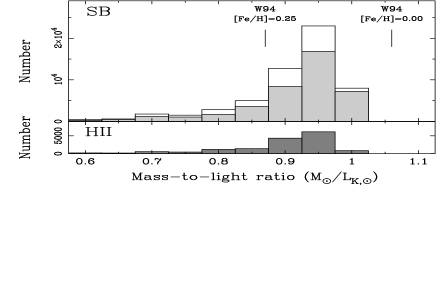
Figure 5: $K$-band mass-to-light ratio frequency histogram. The upper panel shows the distribution for the whole sample (open histogram) and SB-like objects (light-grey filled histogram). The lower-panel shows the frequency histogram of the HII-like galaxies (dark-grey filled histogram). Mass-to-light ratios for model ellipticals with different metallicities are taken from worthey (1994, w94).

The distribution of stellar masses is shown in Figure 4c. This frequency histogram indicates that a typical star forming galaxy in our Local Universe has a stellar mass of about 5$\times$10¹⁰ M_☉. This value is somewhat lower than the stellar mass expected for a local L^∗ galaxy. Assuming M${}^{*}_{K}$=$-$25.1 (for H₀=50 km s^-1 Mpc^-1; Mobasher, Sharples and Ellis, 1993) and a $K$-band mass-to-light ratio of 1 M_☉/L_K,☉ [Héraudeau & Simien 1997], the stellar mass inferred for an L^∗ galaxy is about 2$\times$10¹¹ M_☉. Thus, star-forming galaxies in the local universe are typically a factor 4 less massive than L^∗ galaxies.

In addition, a clear offset between the stellar mass histograms of the SB and HII-like objects is seen in Figure 4c. The distributions of their stellar masses are centred at 7$\times$10¹⁰ and 2$\times$10¹⁰ M_☉ respectively (Figure 4c). This difference is even more significant, about 1 dex, when DHIIH and BCD spectroscopic types (Dwarfs in Table LABEL:resmean) and SBN galaxies are compared. A K-S test analysis of the SB-like and HII-like objects indicates that these two samples come from different age, burst strength and stellar mass distributions with probabilities 98.8, 77.1 and 99.9 per cent respectively.

In Table LABEL:resmean we also present the mean properties that would be obtained using $E(B-V)_{\mathrm{continuum}}=E(B-V)_{\mathrm{gas}}$. In this case, although we obtain important differences in age and burst strength, very similar stellar masses are derived since the stellar mass depends mainly on the $K$-band magnitude, only weakly affected by extinction.

Table 5: Mean and median log($L_{\mathrm{H}\alpha}$/SFR) ratios obtained for different metallicities.

Metallicity	log ($L_{\mathrm{H}\alpha}$/SFR)
$Z$	Mean	Median	Std.dev.
1/50 Z☉	40.19	40.09	0.58
1/5 Z☉	40.38	40.35	0.36
2/5 Z☉	40.31	40.27	0.29
Z☉	40.24	40.29	0.31
2 Z☉	40.19	40.21	0.34
All $Z$	40.23	40.23	0.44

Table 6: Mean SFR and specific SFR for the sample, together with the corresponding standard deviations of the mean. Dwarfs includes DHIIH and BCD spectroscopic type galaxies.

	n	log(SFR)   $\sigma$	log(SFR/M)   $\sigma$
		(M☉ yr-1)	(10-11 yr-1)
Total	67	1.52       0.05	1.81        0.04
SBN	41	1.64       0.06	1.73        0.05
DANS	8	1.21       0.09	1.66        0.09
HIIH	13	1.60       0.08	2.16        0.07
Dwarfs	5	0.82       0.09	1.88        0.14
SB	49	1.57       0.05	1.72        0.04
HII	18	1.38       0.10	2.08        0.07

Figure 6: log ($L_{\mathrm{H}\alpha}$/SFR) frequency histograms for different metallicities and for the whole distribution. Thick marks give the position of the distribution median values.

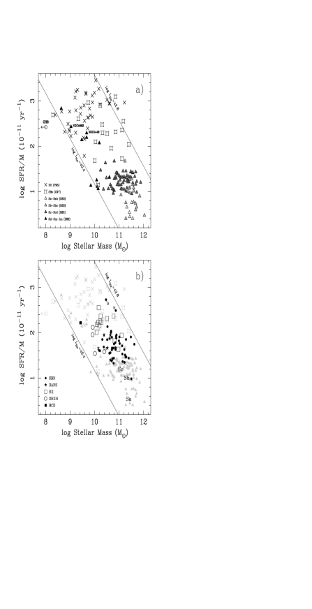
Figure 7: Stellar mass (in M_☉) vs. specific SFR (in 10^-11 yr^-1). a) Dynamical masses from Telles (1995), converted to stellar masses using a correction factor of 0.6 dex. Starburst galaxies from Calzetti (1997b) are also plotted. Data for spiral galaxies have been taken from Kennicutt (1983). b) SBN, DANS, HII, DHIIH and BCD UCM galaxies as classified by Gallego et al. (1996) are plotted. Straight lines define the limits in the H$\alpha$ luminosity function of the UCM survey.

5.6 Star formation rates

Since the star formation activity in the UCM galaxies is better described as a succession of episodic star formation events rather than continuous star formation (see also AH96), the current star formation rate (SFR) is not a meaningful quantity: the latest star formation event might have finished in many of the galaxies, and their current SFR would be zero. However, these galaxies have substantial H$\alpha$ luminosities, and it is accepted that the H$\alpha$ luminosity is a good measurement of the current SFR. In AH96 we showed that this is true, in a statistical sense, for a population of galaxies undergoing a series of star formation events, and we defined an ‘effective’ present-day SFR which coincides with the SFR we would derive if the galaxies were forming stars at a constant rate, producing the same mass in new stars as the ensemble of all the star-formation episodes (see AH96 for details). Here we will follow the same approach.

When estimating star formation rates (SFRs) in AH96 we used the BC93 models and a Salpeter IMF. In the present work, we have used the updated BC96 models with a Scalo IMF. Since the number of Lyman photons (N_Ly) predicted by the old models is about 0.94 dex higher than that predicted by the new ones (for solar metallicity and ages lower than 16 Myr), we need to re-compute the relation between the H$\alpha$ luminosity, $L_{\mathrm{H}\alpha}$, and star formation rate. In addition, we will investigate the change produced in this relation using different metallicity models.

In order to compute the $L_{\mathrm{H}\alpha}$/SFR ratio, we have used a very similar procedure to that employed by AH96: we simulated a population of galaxies undergoing random bursts of star-formation and computed their total H$\alpha$ luminosities and the mass in newly-formed stars. However, instead of considering a uniform age and burst strength probability distribution, we have considered the burst strength, age and metallicity distributions for our galaxy sample. We used 67$\times$1000 points in order to reproduce this distribution in our Monte Carlo simulations. The SFR was computed as the ratio between the stellar mass produced in the burst, i.e. $b$$\times$M, and the maximum age for which we could have detected the galaxy in the UCM sample, that is, the time while EW(H$\alpha$)$>$20Å [Gallego 1995]. The $L_{\mathrm{H}\alpha}$/SFR ratios obtained are shown in Figure 6 for different metallicities and for the total ($t$,$b$,$Z$) distribution. The mean, median, and standard deviation values are given in Table LABEL:fig6t.

Since the changes in this ratio for different metallicity models are quite small, we have adopted the median value of the whole distribution in order to determine the ’effective’ SFR of the galaxies from our sample. The difference between the value adopted here and that of AH96 is about 1 dex, which is very close to the difference in the number of Lyman photons predicted by the BC93 and BC96 models, as expected.

Therefore, we have evaluated the current ’effective’ SFR using the expression

$$\mathrm{SFR}={L_{\mathrm{H}\alpha}\over 1.7\times 10^{40}\mathrm{erg}\,\mathrm{s}^{-1}}\ \ \ \ \mathrm{M}_{\sun}\,\mathrm{yr}^{-1}$$ (4)

This expression assumes that every Lyman photon emitted effectively ionizes the surrounding gas. If, however, as is suggested in Section 5.4, we consider a fraction of non-ionizing Lyman photons of 25 per cent, the star formation rates computed should be 0.1 dex higher.

Specific star formation rates (SFR per unit mass; Guzmán et al. 1997) have been obtained using these SFR values and the stellar masses given by the highest probability solution cluster in Table LABEL:tablafin. The mean SFR and specific SFR for SB-like, HII-like, and whole sample are given in Table LABEL:tablasfrs (see also Figure 4d).

The specific SFR vs. stellar mass diagram is shown in Figure 7 (see Guzmán et al. 1997). In panel-a we show the stellar masses and star formation rates per unit mass for three reference samples. We have included the sample of Kennicutt (1983, K83 hereafter), taking the H$\alpha$ and $B$-band luminosities given by K83 and the stellar mass-to-light ratios of Faber & Gallagher [Faber & Gallagher 1979]. In addition, the sample of HII-galaxies of Telles [Telles 1995] was included, after converting virial masses to stellar masses using a correction of 0.6 dex (Gallego et al. 1999, in preparation) and assuming the H$\beta$-to-H$\alpha$ luminosity ratios used by Guzmán et al. [Guzmán et al. 1997] for this sample. Masses and specific SFRs for the Calzetti [Calzetti 1997b] sample are also shown. In this case, stellar masses were inferred subtracting the HI mass from the dynamical mass measured. The SFR values for the Calzetti [Calzetti 1997b] sample were obtained from their Br$\gamma$ luminosities assuming $L_{\mathrm{H}\alpha}$=102.8$\times$$L_{\mathrm{Br}\gamma}$ (Osterbrook 1989, for $T_{e}$=10⁴ K and $n_{e}$=100 cm^-3). Finally, the dwarf irregular galaxy GR8 [Reaves 1956] was included. Its H$\alpha$ luminosity was obtained from the H$\beta$ luminosity given by Gallagher, Hunter & Bushouse [Gallagher, Hunter & Bushouse 1989], assuming $L_{\mathrm{H}\alpha}$/$L_{\mathrm{H}\beta}$=2.86, and its stellar mass, 3.2$\times$10⁶ M_☉, from Carignan, Beaulieu & Freeman [Carignan, Beaulieu & Freeman 1990]. The limits in the H$\alpha$ luminosity function of Gallego et al. [Gallego et al. 1995], 10^40.4–10^42.8 erg s^-1, are also drawn.

Figure 7 shows that the UCM sample clearly represents a bridge between relaxed spiral galaxies and the most extreme HII galaxies from Telles [Telles 1995], that is, Sp$\rightarrow$SB-like$\rightarrow$HII-like$\rightarrow$HII galaxies. In fact, some of the HII galaxies from Telles [Telles 1995] have very similar properties to those of the less massive HII-like UCM galaxies, mainly DHIIH and BCD spectroscopic types, very rare in our sample (see section 5.1). In addition, most of the SBN type UCM galaxies seem to be normal late-type spirals with enhanced star formation. This star formation enhancement is about a factor of three, and is due to the ongoing nuclear starburst. Thus, the range in specific SFR spanned by the population of the star-forming galaxies that dominate the SFR in the local universe is (10–10³)$\times$10^-11 yr^-1, from the local relaxed spirals to the most extreme HII galaxies. In fact, this range is not very different from that obtained by Guzmán et al. [Guzmán et al. 1997] for a sample of intermediate/high-$z$ compact galaxies from the HDF. The high specific SFR region, where the HII galaxies from Telles [Telles 1995] are placed, is not very well covered by our sample due to the scarcity of very low-luminosity objects, basically DHIIH and BCD spectroscopic type galaxies, relative to the UCM whole sample.

6 Summary

Using new nIR observations and published optical data for 67 galaxies from the Universidad Complutense de Madrid (UCM) survey, we have derived the main properties of their star-forming events and underlying stellar populations. This sample represents about 35 per cent of the UCM galaxies covering the whole range of absolute magnitudes, H$\alpha$ luminosities and equivalent widths spanned by the survey. Burst strengths and ages, stellar masses, stellar mass-to-light ratios and, to a certain extent, metallicities, have been obtained by comparing the observed $r-J$ and $J-K$ colours, $K$-band magnitudes, and H$\alpha$ equivalent widths and luminosities with those predicted by evolutionary synthesis models. The comparison of the observations with the model predictions was carried out using a maximum-likelihood estimator in combination with Monte Carlo simulations which take into account the observational uncertainties. Our main results are:

1. The star-forming galaxies in the UCM sample (used to determine the SFR density of the local universe), show typical burst strengths of about 2 per cent and stellar masses of 5$\times$10¹⁰ M_☉. The current star formation in these galaxies is taking place in discrete star formation events rather than in a continuous fashion. If this is typical of the past star-formation history in the galaxies, many of such star formation events would be necessary to build up their stellar mass. However, our observations provide very little information on star-formation episodes that took place before the current one.

2. We have identified two separate classes of star-forming galaxies in the UCM sample: SB-like and HII-like galaxies. Within the HII-like class the DHIIH and BCD spectroscopic type galaxies, i.e. dwarfs, constitute the most extreme case. The mean burst strength deduced for the SB-like galaxies is about a 25 per cent lower than for the dwarf HII-like galaxies. The average stellar mass is an order of magnitude larger in the former than in the latter. The SB-like galaxies are relatively massive galaxies where the current star formation episode is a minor event in the build up of their stellar masses, while HII-like galaxies are less massive systems in which the present star formation could dominate in some cases their observed properties and contributes to a greater extent to their stellar population.

3. Because of the low burst strengths inferred, $K$-band luminosity is dominated by the old stellar populations, and the $K$-band stellar mass-to-light ratio is almost the same (within $\sim$20 per cent) for all the galaxies. Thus, the $K$-band luminosity is a very good estimator of the stellar mass for typical star-forming galaxies.

4. The average SFR of the galaxies is log(SFR)$\simeq$1.5, with the SFR expressed in M_☉ yr^-1, and it is similar for the SB-like and the HII-like galaxies. However, since the latter are typically less massive, their specific SFR (SFR per unit stellar mass) is significantly larger, in a factor 2.3, than that of the former.

5. The UCM galaxies represent a bridge in specific SFR between relaxed spirals and extreme HII galaxies. The range in specific star formation rate spanned by the local star-forming galaxies, (10–10³)$\times$10^-11 yr^-1, is very similar to that observed in higher redshift objects.

APPENDIX: Analysis of the space of solutions

In this appendix we briefly describe the analysis performed onto the ($t$,log $b$,log $Z$) space of solutions. For each galaxy we have 10³ ($t$,log $b$,log $Z$) points that correspond to the 10³ points generated in the ($r-J$,$J-K$,2.5$\times$log EW(H$\alpha$)) space using a Monte Carlo simulation method.

The mean values ($<t>$,$<$log $b$$>$,$<$log $Z$$>$) are primary indicators of the best ($t$,log $b$,log $Z$) solution, and their standard deviations ($\sigma_{t}$,$\sigma_{\mathrm{log}\,b}$,$\sigma_{\mathrm{log}\,Z}$) could be taken as estimators of the deviation of the data. However, due to the well known age-metallicity and age-burst strength degeneracies these standard deviations are not representative of the distribution of these solutions in the ($t$,log $b$,log $Z$) space. Fortunately, these degenaracies do not span the whole range in age, burst strength and metallicity given by the models, being relatively well constrained by the ($r-J$,$J-K$,2.5$\times$log EW(H$\alpha$)) data.

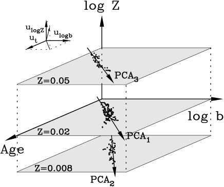
Figure 8: Hypothetical distribution of ($t$,log $b$,log $Z$) solutions. PCA1, PCA2, PCA3 are the principal components for each of the three solution clusters.

Therefore, we have studied the clustering of the ($t$,log $b$,log $Z$) solutions for each individual galaxy. We have used for this analysis a single linkage hierarchical clustering method [Murtagh & Heck 1987]. First, (1) we determine the distances between every couple of solutions, which represents a total of $N\times(N-1)/2$ dissimilarities (=distances), being N the number of solutions. The dissimilarity between the elements $j$ and $k$, $d_{j,k}$, is defined as

$$d_{j,k}^{2}=\sum_{i=1}^{n}(x_{ij}-x_{ik})^{2}$$ (5)

The matrix of dissimilarities is known as dendogram. Then, (2) we find the smallest dissimilarity, $d_{ik}$. These points, $i$ and $k$, (3) are therefore agglomerated and replaced with a new point, $i\cup k$, and the dissimilarities updated such that, for all objects $j\neq i,k$,

$$d_{i\cup k,j}=min\ \{d_{i,j},d_{k,j}\}$$ (6)

Then, (4) the dissimilarities $d_{i,j}$ and $d_{k,j}$, for all $j$, are deleted, as these are no longer used. Finally, we return to step (1) after reducing the dimension of the dissimilarities matrix and the number of clusters. Finally, we recover the last three clusters of solutions.

The clustering pattern obtained is basically produced by the discretization in metallicity of the original BC96 evolutionary synthesis models. Now, we analyze the solutions within each solution cluster. In this case, the discretizations in burst strength and age are comparable and a Principal Component Analysis (PCA hereafter) is the most suitable choice (0.04 dex in burst strength and $\sim$0.05 dex in age).

The PCA basically determines, in a Rⁿ data array, the set of $n$ orthogonal axes that better reproduces our data distribution. The first new axis, i.e. the principal component, will try to go as close as possible through all the data points, describing the larger fraction of the data variance. Figure 8 shows the principal component for each of the three solution clusters of a hypothetical ($t$,log $b$,log $Z$) distribution.

Formally, following the PCA (see, e.g., Morrison 1976), (1) we construct the variance-covariance and the correlation matrix of the sample, being the $(j,k)^{th}$ term of these matrixes, respectively,

$$c_{jk}={1\over n}\sum_{i=1}^{n}(r_{ij}-\overline{r}_{j})(r_{ik}-\overline{r}_{k})$$ (7)

$$\rho_{jk}={1\over n}\sum_{i=1}^{n}{{(r_{ij}-\overline{r}_{j})(r_{ik}-\overline{r}_{k})}\over{s_{j}s_{k}}}$$ (8)

where

$$s_{j}^{2}={1\over n}\sum_{i=1}^{n}(r_{ij}-\overline{r}_{j})^{2}.$$ (9)

Then, (2) solving the eigenvector equation, $\rho u$=$\lambda u$, we obtain the eigenvalues and eigenvectors of the correlation matrix. The ratio between an eigenvalue and the sum of all the eigenvalues, $\lambda_{i}/\sum_{i=1}^{n}\lambda_{i}$, gives us the contribution of the new axis, determined by the corresponding eigenvector, to the total data variance. Therefore, the eigenvector with higher eigenvalue is the principal component and will indicate which is the dominant degeneracy inside each solution cluster.

References

- [Abraham et al. 1999] Abraham R. G., Ellis R. S., Fabian A. C., Tanvir N. R., Glazebrook K., 1999, MNRAS, 303, 641
- [Alonso et al. 1995] Alonso O., Zamorano J., Rego M., Gallego J., 1995, A&AS, 113, 399
- [Alonso et al. 1999] Alonso O., García-Dabó C. E., Zamorano J., Gallego J., Rego M., 1999, ApJS, 122, 415
- [Alonso-Herrero et al. 1996] Alonso-Herrero A., Aragón-Salamanca A., Zamorano J., Rego M., 1996, MNRAS, 278, 417 (AH96)
- [Aragón-Salamanca et al. 1993] Aragón-Salamanca A., Ellis R. S., Couch W. J., Carter D., 1993, MNRAS, 262, 764
- [Armand et al. 1996] Armand C., Baluteau J.-P., Joubert M., Gry C., Cox P., 1996, A&A, 306, 593
- [Balzano 1983] Balzano V. A., 1983, ApJ, 268, 602
- [Barger et al. 1998] Barger A. J. et al., 1998, Nature, 394, 24
- [Baugh et al. 1998] Baugh C. M., Cole S., Frenk C. S., Lacey C. G., 1998, ApJ, 498, 504
- [Bernasconi & Maeder 1996] Bernasconi P. A., Maeder A., 1996, A&A, 307, 829
- [Bershady et al. 1998] Bershady M. A., Haynes M. P., Giovanelli R., Andersen D. R., 1999, in Galaxy Dynamics, ASP conference series, 146, 235
- [Bland-Hawthorn & Maloney 1997] Bland-Hawthorn J., Maloney P. R., 1997, PASA, 14, 59
- [Brocklehurst 1971] Brocklehurst M., 1971, MNRAS, 153, 471
- [Bruzual & Charlot 1993] Bruzual A. G., Charlot S., 1993, ApJ, 405, 538 (BC93)
- [Calzetti et al. 1996] Calzetti D., Kinney A. L., Storchi-Bergmann, T., 1996, ApJ, 458, 132
- [Calzetti 1997a] Calzetti D., 1997a, in Waller H. et al., eds, AIP Conf. Proceedings, Vol.408, The Ultraviolet Universe at Low and High Redshift: Probing the Progress of Galaxy Evolution. American Institute of Physics, New York, p. 403
- [Calzetti 1997b] Calzetti D., 1997b, AJ, 113, 162
- [Cardelli et al. 1989] Cardelli J. A., Clayton G. C., Mathis J. S., 1989, ApJ, 345, 245
- [Carignan, Beaulieu & Freeman 1990] Carignan C., Beaulieu S., Freeman K. C., 1990, AJ, 99, 178
- [Charlot 1998] Charlot S., 1998, in Benvenuti P. et al., eds., The Next Generation Space Telescope: Science Drivers and Technological Challenges, 34th Liége Astrophysics Colloquium, ESA-SP, 429, 135
- [Connolly et al. 1997] Connolly A. J., Szalay A. S., Dickinson M., Subbarao M. U., Brunner R. J., 1997, ApJ, 476, L11
- [Courteau 1995] Courteau S., A compilation of the UKIRT Faint JHK Standars, NOAO, 1995
- [Coziol 1996] Coziol R., 1996, A&A, 309, 345
- [Driver, Windhorst & Griffiths 1995 1995] Driver S. P., Windhorst R. A., Griffiths R. E., 1995, ApJ, 453, 48
- [Elias et al. 1982] Elias J. H., Frogel J. A., Matthews K., Neugebauer G., 1982, AJ, 87, 1029
- [Ellis 1997] Ellis R. S., 1997, ARA&A, 35, 389
- [Faber & Gallagher 1979] Faber S. M., Gallagher J. S., 1979, ARA&A, 17, 135
- [Fernie 1983] Fernie J. D., 1983, PASP, 95, 782
- [Fioc & Rocca-Volmerange 1999] Fioc M., Rocca-Volmerange B., 1999, A&A, 344, 393
- [Gallagher, Hunter & Bushouse 1989] Gallagher J. S., Hunter D. A., Bushouse H., 1989, AJ, 97, 700
- [Gallego 1995] Gallego J., 1995, Ph.D. thesis, Universidad Complutense de Madrid
- [Gallego et al. 1995] Gallego J., Zamorano J., Aragón-Salamanca A., Rego M., 1995, ApJ, 455, L1
- [Gallego et al. 1996] Gallego J., Zamorano J., Rego M., Alonso O., Vitores A. G., 1996, A&AS, 120, 323 (GAL96)
- [Gallego et al. 1997] Gallego J., Zamorano J., Rego M., Vitores A. G., 1997, ApJ, 475, 502
- [Gallego 1998] Gallego J., 1998, in Thuan T. X., Balkowski C., Cayette V., Tran Tranh Van J., eds., Dwarf Galaxies and Cosmology. Proceedings of the XVIIIth Moriond astrophysics meeting, Editions Frontieres. Gif-sur-Yvette, France
- [Glazebrook et al. 1999] Glazebrook K., Blake C., Economou F., Lilly S., Colless M., 1999, MNRAS, 306, 843
- [Guzmán et al. 1996] Guzmán R., Koo D. C., Faber S. M., Illingworth G. D., Takamiya M., Kron R. G., Bershady M. A., 1996, ApJ, 460, L5
- [Guzmán et al. 1997] Guzmán R. et al., 1997, ApJ, 489, 559
- [Hammer et al. 1997] Hammer F. et al., 1997, ApJ, 481, 49
- [Héraudeau & Simien 1997] Héraudeau P., Simien F., 1997, A&A, 326, 897
- [Herbst et al. 1993] Herbst T. M., Beckwith S. V., Birk C., Hippler S., McCaughrean M. J., Mannucci F., Wolf J., 1993, in Fowler A. M., ed., Proc. SPIE, Vol. 1946, Infrared Detectors and Instrumentation. The International Society for Optical Engineering, p.605
- [Hu, Cowie & McMahon 1998] Hu E. M., Cowie L., McMahon R. G., 1998, ApJ, 502, 99
- [Hughes et al. 1998] Hughes D. et al., 1998, Nature, 394, 241
- [Kennicutt 1983] Kennicutt R. C., 1983, ApJ, 272, 54
- [Kennicutt 1992] Kennicutt R. C., 1992, ApJ, 388, 310
- [Kent 1985] Kent S. M., 1985, PASP, 97, 165
- [Krüger, Fritze-v. Alvensleben & Loose 1995] Krüger H., Fritze-v. Alvensleben U., Loose H.-H., 1995, A&A, 303, 41
- [Leitherer et al. 1995] Leitherer C., Ferguson H. C., Heckman T. M., Lowenthal J. D., 1995, ApJ, 454, L19
- [Lilly et al. 1995] Lilly S. J., Le Fevre O., Crampton D., Hammer F., Tresse L., 1995, ApJ, 455, 60
- [Lilly et al. 1998] Lilly S. J. et al., 1998, ApJ, 500, 75
- [Lowenthal et al. 1997] Lowenthal J. D., Koo D. C., Guzmán R., Gallego J., Phillips A. C., Faber S. M., Vogt N. P., Illingworth G. D., Gronwall C., 1997, ApJ, 481, 673
- [Madau 1997] Madau P., 1997, in Holt S. S. & Mundy L. G., eds., AIP Conf. Proceedings, Vol.393, Star Formation Near and Far. American Institute of Physics, New York, p.481
- [Madau et al. 1996] Madau P., Ferguson H. C., Dickinson M. E., Giavalisco M., Steidel C. C., Fruchter A., 1996, MNRAS, 283, 1388
- [Madau et al. 1998] Madau P., Dickinson M. E., Pozzeti L., 1998, ApJ, 498, 106
- [Mathis 1990] Mathis J. S., 1990, ARA&A, 28, 37
- [Misch et al. 1995] Misch A., Gilmore K., Rank D., 1995, UCO-Lick Technical Reports, 77, Sta. Cruz, California
- [Mobasher et al. 1993] Mobasher B., Sharples R. M., Ellis R. S., 1993, MNRAS, 263, 560
- [Morrison 1976] Morrison D. F., 1976, Multivariate Statistical Methods, McGraw-Hill Book Co., Singapore
- [Murtagh & Heck 1987] Murtagh F., Heck A., 1987, Multivariate Data Analysis, D. Reidel Publishing Co., Dordrecht, Holland
- [Osterbrock 1989] Osterbrock D. E., 1989, Astrophysics of Gaseous Nebulae and Active Galactic Nuclei. University Science Books, Mill Valley, California
- [Pei & Fall 1995] Pei Y. C., Fall S. M., 1995, ApJ, 454, 69
- [Peletier & Balcells 1996] Peletier R. F., Balcells M., 1996, AJ, 111, 2238
- [Poggianti 1997] Poggianti B. M., 1997, A&AS, 122, 399
- [Reaves 1956] Reaves G., 1956, AJ, 61, 69
- [Rowan-Robinson et al. 1997] Rowan-Robinson M. et al., 1997, MNRAS, 289, 490
- [Salzer et al. 1989] Salzer J. J., MacAlpine G. M., Boroson T. A., 1989, ApJS, 70, 479
- [Scalo 1986] Scalo J. M., 1986, Fund. Cosmic Phys., 11, 1
- [Somerville et al. 1999] Somerville R. S., Primack J. R., Faber S. M., 1999, MNRAS, in press
- [Steidel et al. 1996] Steidel C. C., Giavaliso M., Pettini M., Dickinson M., Adelberger K. L., 1996, ApJ, 462, 17
- [Steidel et al. 1999] Steidel C. C., Adelberger K. L., Giavaliso M., Dickinson M., Pettini M., 1999, ApJ, 519, 1
- [Storchi-Bergmann, Calzetti & Kinney 1994] Storchi-Bergmann T., Calzetti D., Kinney A. L., 1994, ApJ, 429, 572
- [Telles 1995] Telles E., 1995, Ph.D. thesis, Cambridge University
- [Thuan & Gunn 1976] Thuan T. X., Gunn J. E., 1976, PASP, 88, 543
- [Tresse & Maddox 1998] Tresse L., Maddox S. J., 1998, ApJ, 495, 691
- [Treyer et al. 1998] Treyer M. A., Ellis R. S., Milliard B., Donas J., Bridges T. J., 1998, MNRAS, 300, 303
- [Vitores 1994] Vitores A. G., 1994, Ph.D. thesis, Universidad Complutense de Madrid
- [Vitores et al. 1996a] Vitores A. G., Zamorano J., Rego M., Alonso O., Gallego J., 1996a, A&AS, 118, 7
- [Vitores et al. 1996b] Vitores A. G., Zamorano J., Rego M., Gallego J., Alonso O., 1996b, A&AS, 120, 385
- [Wainscoat & Cowie 1992] Wainscoat R. J., Cowie L. L., 1992, AJ, 103, 332
- [Williams et al. 1996] Williams R. E. et al., 1996, AJ, 112, 1335
- [Worthey 1994] Worthey G., 1994, ApJS, 95, 107
- [Zamorano et al. 1994] Zamorano J., Rego M., Gallego J., Vitores A. G., González-Riestra R., Rodríguez G., 1994, ApJS, 95, 387
- [Zamorano et al. 1996] Zamorano J., Gallego J., Rego M., Vitores A. G., Alonso O., 1996, ApJS, 462, 1