CMB $B$-polarization to map the Large-scale Structures of the Universe

Abstract

We explore the possibility of using the $B$-type polarization of the Cosmic Microwave Background to map the large-scale structures of the Universe taking advantage of the lens effects on the CMB polarization. The functional relation between the $B$ component with the primordial CMB polarization and the line-of-sight mass distribution is explicited. Noting that a sizeable fraction (at least 40%) of the dark halo population which is responsible of this effect can also be detected in galaxy weak lensing survey, we present statistical quantities that should exhibit a strong sensitivity to this overlapping. We stress that it would be a sound test of the gravitational instability picture, independent on many systematic effects that may hamper lensing detection in CMB or galaxy survey alone. Moreover we estimate the intrinsic cosmic variance of the amplitude of this effect to be less than 8% for a $100\,\textrm{deg}^{2}$ survey with a $10^{\prime}$ CMB beam. Its measurement would then provide us with an original mean for constraining the cosmological parameters, more particularly, as it turns out, the cosmological constant $\Lambda$.

]

I Introduction

In the new era of precision cosmology we are entering in, the forthcoming experiments will provides us with accurate data on Cosmic Microwave Background anisotropies[1]. This should lead to accurate determinations of the cosmological parameters, provided the large-scale structures of the Universe indeed formed from gravitational instabilities of initial adiabatic scalar perturbations. It has been soon realized however that even with the most precise experiments, the cosmological parameter space is degenerate when the primary CMB anisotropies alone are considered[2]. Complementary data, that may be subject to more uncontrollable systematics are thus required, such as supernovae surveys[3] (but see [4]) or constraints derived from the large-scale structure properties. Among the latter, weak lensing surveys are probably the safer[5], but still have not yet proved to be accurate enough with the present day observations.

Secondary CMB anisotropies (i.e. induced by a subsequent interaction of the photons with the mass or matter fluctuations) offer opportunities for raising this degeneracy. Lens effects[6] are particularly attractive since they are expected to be one of the most important.They also are entirely driven by the properties of the dark matter fluctuations, the physics of which involve only gravitational dynamics, and are therefore totally controlled by the cosmological parameters and not by details on galaxy or star formation rates. More importantly an unambiguous detection of the lens effects on CMB maps would be a precious confirmation of the gravitational instability picture. Methods to detect the lens effects on CMB maps have been proposed recently. High order correlation functions[7], peak ellipticities[8] or large scale lens induced correlators[9] have been proposed for detecting such effects. All of them are however very sensitive to cosmic variance since lens effect is only a sub-dominant alteration of the CMB temperature patterns. The situation is different when one considers the polarization properties. The reason is that in standard cosmological models temperature fluctuations at small scale are dominated by scalar perturbations. Therefore the pseudo-scalar part, the so called $B$ component, of the polarization is negligible compared to its scalar part (the $E$ component) and can only be significant when CMB lens couplings are present. This mechanism has been recognized in earlier papers[10, 11]. The aim of this paper is to study systematically the properties of the lens induced B field and uncover its properties.

In section II, we perturbatively compute the lens effect on the CMB polarization $E$ and $B$ field. This first order equation is illustrated by numerical experiments. Possibility of direct reconstruction of the projected mass distribution is also examined. As it has already been noted a significant fraction of the potential wells that deflect the CMB photons can actually be mapped in local weak lensing surveys[12, 13]. This feature has been considered so far in relation to the CMB temperature fluctuations. We extend in Section III these studies to the CMB polarization exploiting the specificities of the field found in previous section. In particular we propose two quantities that can be built from weak lensing and Cosmic Microwave Background polarization surveys, the average value of which does not vanish in presence of CMB lens effects. Compared to direct analysis of the CMB polarization, such tools have the joint advantage of being less sensitive to systematics –systematic errors coming from CMB mapping on one side and weak lensing measurement on the other side have no reason to correlate!– and so emerge even in presence of noisy data, and of being an efficient probe of the cosmological constant. Indeed the expected amplitude of correlation is directly sensitive to the relative length of the optical bench, from the galaxy source plane to the CMB plane, which is mainly sensitive to the cosmological constant. Filtering effects and cosmic variance estimation of such quantities are considered in this section as well.

II Lens effects on CMB polarization

II.1 First order effect

Photons emerging from the last scattering surface are deflected by the large scale structures of the Universe that are present on the line-of-sights. Therefore photons observed from apparent direction $\vec{\alpha}$ must have left the last scattering surface from a slightly different direction, $\vec{\alpha}+\vec{\xi}(\vec{\alpha})$, where $\vec{\xi}$ is the lens induced apparent displacement at that distance. The displacement field is related to the angular gradient of the projected gravitational potential. In the following, the lens effect will be described by the deformation effects it induces, encoded in the amplification matrix,

$${\cal A}^{-1} = \left(\begin{array}[]{cc}1-\kappa-\gamma_{1}&-\gamma_{2}\\ -\gamma_{2}&1-\kappa+\gamma_{1}\end{array}\right)$$ (3)

$$= \delta_{i}^{j}+\xi^{j}_{,i}$$ (4)

so that

$$\kappa = -\frac{1}{2}(\xi^{x}_{,x}+\xi_{,y}^{y})$$

$$\gamma_{1} = -\frac{1}{2}(\xi^{x}_{,x}-\xi_{,y}^{y})$$

$$\gamma_{2} = -\xi_{,x}^{y}=-\xi_{,y}^{x}.$$ (5)

The lens effect affects the local polarization just by moving the apparent direction of the line of sight[15]. Thus, if we use the Stokes parameters $Q$ and $U$ to describe the local polarization vector,

$$\vec{P}=\left(\begin{array}[]{c}Q\\ U\end{array}\right)$$

we can relate the observed polarization $\hat{\vec{P}}$ to the primordial one by the relation

$$\hat{Q}(\vec{\alpha})=Q(\vec{\alpha}+\vec{\xi}),\qquad\hat{U}(\vec{\alpha})=U(\vec{\alpha}+\vec{\xi}).$$ (6)

From now on we will denote $\hat{x}$ an observed quantity and $x$ the primordial one. $\overrightarrow{\alpha}^{\prime}=\vec{\alpha}+\vec{\xi}$ is the sky coordinate system for the observer, therefore the amplification matrix ${\cal A}$ is also the Jacobian of the transformation between the source plane and the image plane. We will restrain here our computation to the weak lensing effect so observed quantity will not take into account any other secondary effect. It is very important at this point to note that the lensing effect does not produce any polarization nor rotate the Stokes parameter. In this regime its effect reduces to a simple deformation of the polarization patterns, similar to the temperature maps. This is the mechanism by which the geometrical properties of the polarization field are changed.

To see that we have to consider the electric ($E$) and magnetic ($B$) components instead of the Stokes parameters. At small angular scales (we assume that a small fraction of the sky can be described by a plane), these two quantities are defined as,

$$E \equiv \Delta^{-1}\left[\left(\partial_{x}^{2}-\partial_{y}^{2}\right)\,Q+2\partial_{x}\partial_{y}\,U\right]$$ (7)

$$B \equiv \Delta^{-1}\left[\left(\partial_{x}^{2}-\partial_{y}^{2}\right)\,U-2\partial_{x}\partial_{y}\,Q\right].$$

This fields reflect non-local geometrical properties of the polarization field. The electric component accounts for the scalar part of the polarization and the magnetic one, the pseudo-scalar part: by parity change $E$ is conserved, whereas $B$ sign is changed. As it has been pointed out in previous papers[10, 11, 14], lens effects partly redistribute polarization power in these two fields.

We explicit this latter effect in the weak lensing regime where distortions, $\kappa$ and $\gamma_{i}$ components are small. This is indeed expected to be the case when lens effects by the large-scale structures are considered, for which the typical value of the convergence field $\kappa$ is expected to be $\sim 1\%$ at 1 degree scale. The leading order effect is obtained by simply pluging (6) in (7) and by expanding the result at leading order in $\xi$ , $\kappa$, and $\gamma$ . Noting that (these calculations are very similar to those done in [13]),

$$\partial_{i}\hat{X} = \widehat{\partial_{k}X}\cdot\left(\delta_{i}^{k}+\xi^{k}_{,i}\right)$$ (8)

$$\partial_{i}\partial_{j}\hat{X} = \widehat{\partial_{k}\partial_{l}X}\cdot(\delta_{i}^{k}+\xi^{k}_{,i})(\delta_{j}^{l}+\xi_{,j}^{l})$$

$$\qquad+\widehat{\partial_{k}X}\cdot\xi_{,ij}^{k}$$

we can write a perturbation description of the lensing effect on electric and magnetic components of the polarization. At leading order one obtains:

$$\Delta\hat{E} = \Delta E+\xi^{i}\partial_{i}\Delta E-2\kappa\Delta E$$

$$\quad-2\delta_{ij}\left(\gamma^{i}\Delta P^{j}+\gamma^{i}_{,k}P^{j,k}\right)+O(\gamma^{2})$$

$$\Delta\hat{B} = \Delta B+\xi^{i}\partial_{i}\Delta B-2\kappa\Delta B$$

$$\quad-2\epsilon_{ij}\left(\gamma^{i}\Delta P^{j}+\gamma^{i}_{,k}P^{j,k}\right)+O(\gamma^{2}),$$

Where we used the fact that $\widehat{\Delta X}=\Delta X+\xi^{i}\partial_{i}\Delta X$ at the leading order. The formulas for $E$ and $B$ are alike. The only difference stands in the $\delta_{ij}$ and $\epsilon_{ij}$ (the latter is the totally antisymmetric tensor, $\epsilon_{11}=\epsilon_{22}=0,$ $\epsilon_{12}=-\epsilon_{21}=1$) that reflects the geometrical properties of the two fields. The first three terms of each of these equations represent the naive effect: the lens induced deformation of the $E$ or $B$ fields. This effect is complemented by an enhancement effect (respectively $\kappa\,\Delta E$ and $\kappa\,\Delta B$) and by shear-polarization mixing terms.The latter effects consist in two parts. One which we will call the ${\tiny\Delta}$-term that couples the shear with second derivative of the polarization field. The other one, hereafter the ${\tiny\nabla}$-term, mixes gradient of the shear and polarization. Although terms like ${\tiny\nabla}$ have been neglected in similar computations[13] we cannot do that here a priori. We will indeed show later that these two terms have similar amplitudes.

One consequence of standard inflationary models on CMB anisotropies is the unbalanced distribution of power between the electric ($E$) and magnetic ($B$) component of its polarization. Adiabatic scalar fluctuations do not induce $B$-type polarization and they dominate at small scales over the tensor perturbations (namely the gravity waves). So, even though gravity waves induce $E$ and $B$ type polarization in a similar amount, primary CMB sky is expected to be completely dominated by $E$ type polarization at small scales. Then for this class of models the actual magnetic component of the polarization field is generated by the corrective part of eq. (II.1),

$$\Delta\hat{B}=-2\epsilon_{ij}\left(\gamma^{i}\Delta\hat{P}^{j}+\gamma^{i}_{,k}\hat{P}^{j,k}\right)$$ (10)

This result extends the direct lens effects described in Benabed & Bernardeau[11] who focused their analysis on the lens effect due to the discontinuity of the polarization field in case of cosmic strings. Previous studies of the weak lensing effect on CMB showed that with lensing, the $B$ component becomes important at small scales[18]. We obtain here the same result but with a different method; eq. (10) means that the polarization signal $P$ is redistributed by the lensing effect in a way that breaks the geometrical properties of the primordial field. Note here that it is mathematically possible to build a shear field that preserves these geometrical properties and that does not create any $B$ signal at small scales. We will discuss this problem in Sec. II.3. It also means that $B$ directly reflects the properties of the shear map. We will take advantage of this feature to probe the correlation properties of $B$ with the projected mass distribution in next sections.

II.2 Lens-induced $B$ maps

We show examples of lens induced $B$ maps. These maps have been calculated using “CMBSlow” code developed by A. Riazuelo (see [19]) to compute primordial polarization maps (we use realizations of standard CDM model to illustrate lens effects). Then various shear maps are applied. We present both true distortions, (obtained by Delaunay triangulation used to shear the $Q$ and $U$ fields), and the first order calculations given by eq. (10).

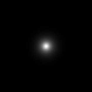
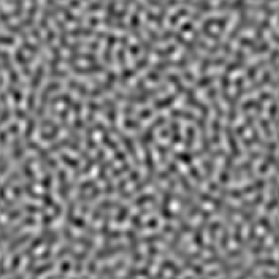
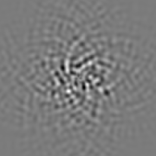
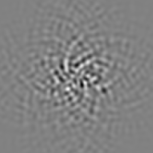
Figure 1: Lens effect induced by a large isothermal sphere with finite core radius. The $\kappa$ map of the lens is shown on left panel. The primordial $E$ sky is presented in the middle left panel. It has been generated for a $\Omega_{0}=0.3$, $\Lambda=0.7$ model, without tensor modes. The middle right panel displays the true reconstructed $\Delta\hat{B}$ field in a $4.5\times 4.5$ degree map and the right panel shows the first order approximation. Note that the rosette-like shape the eye seams to catch in $B$ fields is a numerical coincidence and has no special significance.

Fig. 1 presents the shear effect induced by an isothermal sphere with finite core radius (and the lens edges have been suppressed by an exponential cutoff to minimize numerical noise). The agreement between true distortion (central panel ) and first order formula (right panel) is good. However, a close examination of the maps reveals that some structures in the true map are slightly wider than their counterparts in the first order map. This error is more severe in the center, where the distortion is bigger, which is to be expected since the limits of the validity region of first order calculations are reached.

Fig. 2 shows the $B$ field induced by a realistic distortion. We use second order Lagrangian dynamics[21] to create a $2.5\times 2.5$ degree map that mimics a realistic projected mass density up to $z=1000$ and used its gravitational distortion to compute a typical weak lensing-induced $B$ map. Again we compare the exact effect (i.e. left panel where Delaunay triangulation is used) and the first order formula (middle panel). Right panel shows the difference between the two maps. It reveals the locations where the two significantly disagree. In fact most disagreements are due to slight mismatch of the $B$ patch positions, which lead to dipole like effects in this map.

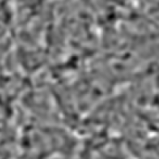
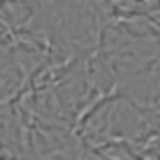
Figure 2: The effect of a realistic weak lensing field on B. $2.2\times 2.2$ degree survey with $1.8^{\prime}$ resolution.The left panel shows exact distortion obtained by Delaunay triangulation. The middle one, the first order formula result, and the right gives the difference between the two. The three panels share the same color table. The mean amplitude in the difference map is about 3 times smaller.

We also show here a comparison of the two parts of the first order formula eq. (10) in order to see which of the ${\tiny\Delta}$ or ${\tiny\nabla}$ terms dominates. It would be more comfortable if one of the two terms was dominant, however, Fig. 3 shows that it is not the case. Even if the ${\tiny\Delta}$-term dominates at low ($<1000)$ $\ell$, it is only twice bigger than ${\tiny\nabla}$-one at this scale. The inverse is true for higher ($3000\sim 5000)$ $\ell$s. This can be seen by looking at Fig. 4 where we show the relative amplitudes of the ${\tiny\Delta}$ and ${\tiny\nabla}$ contributions. The ${\tiny\Delta}$ part gives birth to large patches (around $10^{\prime}$) while ${\tiny\nabla}$ panel shows a lot more of small features.

Figure 3: The $C_{\ell}$ of a $100$ square degree $B$ map. The solid line is the full first order approximation formula. The dotted line gives the contribution of the ${\tiny\nabla}$-term. The dash-dotted one represents the ${\tiny\Delta}$-term. The latter is dominant at small $\ell$s, around $\ell=1000$, that is to say for structures around $10^{\prime}$. The ${\tiny\nabla}$ contribution gives birth to smaller structures in the $1\sim 2$ arc-minute range.

II.3 Direct reconstruction – Kernel problem

The fact that the observable $B$ is at leading order proportional to the weak lensing signal invites us to try a direct reconstruction, similar to the lensing mass reconstruction. In fact, we can write

$$\Delta\hat{B}=-2\epsilon_{ij}\left(\gamma^{i}\Delta\hat{P}^{j}+\gamma^{i}_{,k}\hat{P}^{j,k}\right)\equiv{\mathrm{F}}[\gamma]$$ (11)

and our reconstruction problem becomes an inversion problem for the operator ${\mathrm{F}}$. Unfortunately, one can prove that this problem has no unique solution. It is due to the fact that $\mathrm{F}$ admits a huge kernel, in the sense that, given a polarization map, there is a wide class of shear fields that will conserve a null $B$ polarization. The demonstration of this property is sketched in the following.

Since the unlensed polarization is only electric in our approximation, we can describe it by the Laplacian of a scalar field ;

$$E\equiv\Delta\varphi\textrm{ so }\left\{\begin{array}[]{l}Q=\left(\partial_{x}^{2}-\partial_{y}^{2}\right)\,\varphi\\ U=2\,\partial_{x}\partial_{y}\,\varphi\end{array}.\right.$$ (12)

The same holds for the shear and convergence fields

$$\kappa\equiv\frac{\Delta\psi}{2},\>\gamma_{1}=\frac{1}{2}\left(\partial_{x}^{2}-\partial_{y}^{2}\right)\,\psi\textrm{ },\>\gamma_{2}=\partial_{x}\partial_{y}\,\psi.$$ (13)

Thus we need to know, for a given $\varphi$ field, whether there is any $\psi$ that fulfills the equation

$$\gamma_{2}\,\Delta Q-\gamma_{1}\,\Delta U+\partial_{i}\gamma_{2}\,\partial^{i}Q-\partial_{i}\gamma_{1}\,\partial^{i}U=0.$$ (14)

$\varphi$ and $\psi$ can be written as polynomial decompositions

$$\varphi(x,y) = \sum_{n,l}\,a_{nl}\,x^{n}y^{l}$$

$$\psi(x,y) = \sum_{m,k}\,b_{mk}\,x^{m}y^{k}.$$ (15)

Using (15) in (14) we are left with a new polynomial whose coefficients $c_{ij}$ are sums of $a_{nl}\times b_{mk}$ and have to be all put to zero. With the coefficient equations in hand, it is easy to prove that assuming all the $b_{mk}$ coefficient up to $m+k=N$ are known and writing the equations $\forall\,i+j=(N+1)-3,\,c_{ij}=0$, we can compute out of all the $a_{nl}$ all but three $b_{mk}$ with $m+k=N+1$. This is somewhat similar to mass reconstruction problems from galaxy surveys where one cannot avoid the mass sheet degeneracy. The situation is however worse in our case since not only constant convergence but also translations and a whole class of $a_{nk}$ realization dependent complex deformations are indiscernible. Thus, with the only knowledge of the $B$ component of the polarization one cannot, with the first order eq. (10), recover the projected mass distribution.

III Cross-correlating CMB maps and weak lensing surveys

III.1 Motivations

Even with the most precise experiments it is clear that clean detections of $B$ component will be difficult to obtain. The magnetic polarization amplitude induced with such a mechanism is expected to be one order of magnitude below the electric one[18]. Besides even if we know that there is a window in angular scale where the other secondary effects will not interfere too much with the detection of the lens-induced $B$[23], few is known about removing the foregrounds[22] to obtain clean maps reconstruction algorithms would require.

These considerations lead us to look for complementary data sets to compare $B$ with. Although the source plane for weak lensing surveys[5] is much closer than for the lensed CMB fluctuations, we expect to have a significant overlapping region in the two redshift lens distributions, so that weak lensing surveys can map a fair fraction of the line-of-sight CMB lenses. Consequently, weak lensing surveys can potentially provide us with shear maps correlated with $B$, but which have different geometrical degeneracy, noise sources and systematics than the polarization field.

The correlation strength between the lensing effects at two different redshifts can be evaluated. We define $r$ as the cross-correlation coefficient between two lens planes:

$$r(z_{\mathrm{\textsc{\tiny gal}}})=\frac{\left\langle\kappa\,\kappa_{\mathrm{\textsc{\tiny gal}}}\right\rangle}{\sqrt{\left\langle\kappa^{2}\right\rangle\left\langle\kappa_{\mathrm{\textsc{\tiny gal}}}^{2}\right\rangle}}.$$ (16)

In a broad range of realistic cases (see tab. 1), $r\sim 40\%$. To take advantage of this large overlapping we will consider quantity that cross correlates the CMB $B$ field and galaxy surveys. Moreover, cross-correlation observations are expected to be insensitive to noises in weak lensing surveys and in CMB polarization maps. This idea has already been explored for temperature maps[13]. We extend this study here taking advantage of the specific geometrical dependences uncovered in the previous section.

$r$ coefficient	$z_{\mathrm{\textsc{\tiny gal}}}=1$	$z_{\mathrm{\textsc{\tiny gal}}}=2$
EdS, Linear	0.42	0.60
$\Omega=0.3$, $\Lambda=0.7$, Linear	0.31	0.50
$\Omega=0.3$, $\Lambda=0.7$, Non Linear	0.40	0.59

Table 1: values of $r$, the cross-correlation between two source planes ($z_{\mathrm{\textsc{\tiny gal}}}$ and $z_{\mathrm{\textsc{\tiny cmb}}}=1100$) for different models. The adopted filter scale (see Sect. III.3 for details) is 2 arcmin for both weak lensing survey and Cosmic Microwave Background observations.Non-linear $P(k)$ has been computed using Peacock and Doddsmethod [17].

III.2 Definition of $b_{{\tiny\Delta}}$ and $b_{{\tiny\nabla}}$.

The magnetic component of the polarization in eq. (10) appears to be built from a pure CMB part, which comes from the primordial polarization, and a gravitational lensing part. It is natural to define $b$, in such a way that mimics the $\Delta\hat{B}$ fonction dependance, by replacing the CMB shear field by the galaxy one.

$$b = \epsilon_{ij}\left(\gamma_{\mathrm{\textsc{\tiny gal}}}^{i}\Delta\hat{P}^{j}+\gamma^{i}_{\mathrm{\textsc{\tiny gal}},k}\hat{P}^{j,k}\right)$$

$$= \epsilon_{ij}\left(\gamma_{\mathrm{\textsc{\tiny gal}}}^{i}\Delta P^{j}+\gamma_{\mathrm{\textsc{\tiny gal}},k}^{i}P^{j,k}\right)+O(\kappa^{2}).$$

In the following, we will label local lensing quantities, such as what one can obtain from lensing reconstruction on galaxy surveys, with a gal index. This new quantity can be viewed as a guess for the CMB polarization $B$ component if lensing was turned on only in a redshift range matching the depth of galaxy surveys. The correlation coefficient of this guess with the true $\Delta B$ field, that is $\left\langle\Delta\hat{B}\,b\right\rangle$, is expected to be quadratic both in $P$ and in $\gamma$ and to be proportional to the cross-coefficient $r$.

For convenience, and in order to keep the objects we manipulate as simple as possible, we will not exactly implement this scheme, as it will lead to uneven angular derivative degrees in the two terms of resulting equations. We can, instead, decompose the effect in the ${\tiny\Delta}$ and ${\tiny\nabla}$-part. These two are not correlated, since their components do not share the same degrees of angular derivation. Hence, we can play the proposed game, considering the two terms of eq. (10) as if they were two different fields, creating two guess-quantities that should correlate independently with the observed $B$ field. Following this idea we build $b_{{\tiny\Delta}}$ as,

$$b_{{\tiny\Delta}} \equiv \epsilon_{ij}\gamma_{\mathrm{\textsc{\tiny gal}}}^{i}\Delta\widehat{P}^{j}$$

$$= \epsilon_{ij}\gamma_{\mathrm{\textsc{\tiny gal}}}^{i}\Delta P^{j}+O(\kappa^{2})$$

which corresponds to the ${\tiny\Delta}$-term in eq. (10). The amplitude of the cross-correlation between $\Delta B$ and $b_{{\tiny\Delta}}$ can easily be estimated. At leading order, we have

$$\left\langle\Delta\widehat{B}\,b_{{\tiny\Delta}}\right\rangle=-2\epsilon_{ij}\epsilon_{kl\,}\left\langle\gamma^{k}\gamma^{i}_{\mathrm{\textsc{\tiny gal}}}\right\rangle\left\langle\Delta P^{l}\Delta P^{j}\right\rangle.$$ (19)

The corresponding ${\tiny\nabla}$ correlation is

$$\left\langle\Delta\widehat{B}\,b_{{\tiny\nabla}}\right\rangle=-2\epsilon_{ij}\epsilon_{kl\,}\left\langle\partial_{m}\gamma^{k}\partial_{n}\gamma^{i}_{\mathrm{\textsc{\tiny gal}}}\right\rangle\left\langle\partial_{m}P^{l}\partial_{n}P^{j}\right\rangle$$ (20)

where we have defined

$$b_{{\tiny\nabla}}\equiv\epsilon_{ij}\partial_{k}\gamma_{\mathrm{\textsc{\tiny gal}}}^{i}\partial_{k}\widehat{P}^{j}.$$ (21)

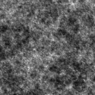
(a)

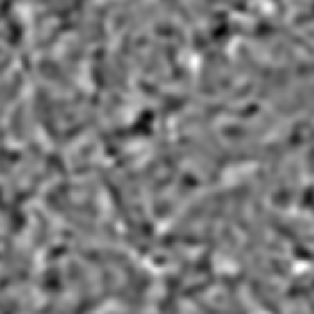
(b)

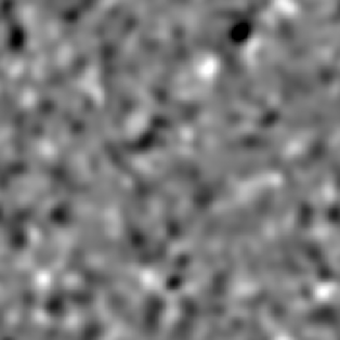
(c)

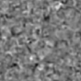
(d)

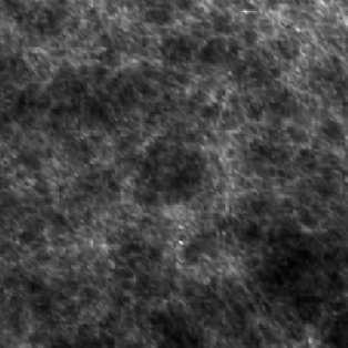
(e)

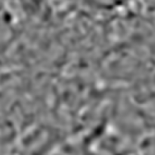
(f)

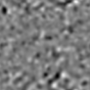
(g)

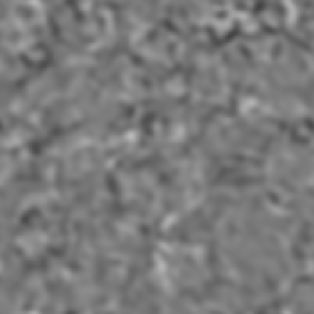
(h)

Figure 4: The effect of the two terms of the perturbation formula. Top row, the lens effect is the sum of the lenses up to recombination. Bottom row, we use the same line -of-sight mass fluctuations but only up to redshift unity, it represent our ’local’ lensing survey. The convergence fields (left panels) have been computed by slicing the $z$-axis and summing up the lensing effect in each slice. Lens-lens coupling (including departure from Born approximation) terms have been neglected, which is consistent with our first order approximation. The convergence in each slice has been created by using second order Lagrangian dynamics. The middle-left panels show the leading order contribution, the middle right the ${\tiny\Delta}$ contribution and the right the ${\tiny\nabla}$ one. In this example, the correlation coefficient between the two convergence maps, $r$ is equal to 0.48 at $1.8^{\prime}$. The cross correlation coefficient between the guess map (f) and the real one (b) is 0.47. It is 0.37 between the real (b) and ${\tiny\Delta}$ (g) maps and goes down to 0.16 for the real (b) and ${\tiny\nabla}$ (h).

Fig. 4 shows numerical simulations presenting maps of first order $\Delta\widehat{B}$, its ${\tiny\Delta}$ and ${\tiny\nabla}$ contributions and the corresponding guess maps one can build with a low $z$ shear map. The similarities between the top maps and the bottom maps are not striking. Yet, under close examination one can recognize individual patterns shared between the maps. This is confirmed by the computation of the correlation coefficient between the maps, that shows significant overlapping, between 50% and 15%, depending correlation and filtering strategy. The calculations hereafter will evaluate the theoretical correlation structure between maps given in figs. 4-b and 4-g & h.

For galaxy surveys, the amplification matrix is[16],

$${\cal A}_{\mathrm{\textsc{\tiny gal}}}^{-1}(\vec{\alpha})-\textrm{Id}=-\int_{0}^{z_{\mathrm{\textsc{\tiny gal}}}}{\mathrm{d}}\chi\,w_{\mathrm{\textsc{\tiny gal}}}(\chi)$$ (22)

$$\qquad\times\int\frac{{\mathrm{d}}^{3}k}{(2\pi)^{\frac{3}{2}}}\delta(\vec{k}){\mathrm{e}}^{{\mathrm{i}}\left(k_{r}\chi+\vec{k}_{\bot}D(\chi)\vec{\alpha}\right)}$$

$$\qquad\times\left(\begin{array}[]{cc}1+\cos(2\phi_{k_{\perp}})&\sin(2\phi_{k_{\perp}})\\ \sin(2\phi_{k_{\perp}})&1-\cos(2\phi_{k_{\perp}})\end{array}\right)$$ (25)

where $\delta(k)$ is the Fourier transform of the density contrast at redshift $z(\chi)$, $w$ is the lens efficiency function, $\mathrm{D}$ is the angular distance, and $\phi_{k_{\perp}}$is the position angle of the transverse wave-vector $k_{\perp}$in the $k_{\perp}=(k_{x},\,\,k_{y})$ plane. Assuming a Dirac source distribution the efficiency function is given by

$$w_{\mathrm{\textsc{\tiny gal}}}(z)=\frac{3}{2}\Omega_{{\mathrm{o}}}\frac{\mathrm{D}_{z}\mathrm{D}_{z\rightarrow z_{\mathrm{\textsc{\tiny gal}}}}}{a\,\mathrm{D}_{z_{\mathrm{\textsc{\tiny gal}}}}}.$$ (26)

Note that the Fourier components $\delta(k)$ include the density time evolution. They are thus proportional to the growth factor in the linear theory. The time evolution of these components is much more complicated in the nonlinear regime (see [17]).

Then, $b_{\natural}$ is

$$b_{\natural}(\vec{\alpha})=\int^{\chi_{\mathrm{\textsc{\tiny gal}}}}{\cal D}(\chi,\vec{l},\vec{k})\,\tilde{E}(l)\,\delta(k)\,{\mathcal{G}}^{\rm Ker}_{\natural}\left(\vec{l},\vec{k}_{\perp}\right)$$ (27)

with the integration element defined as,

$${\cal D}(\chi,\vec{l},\vec{k})={\mathrm{d}}\chi\,w_{\mathrm{\textsc{\tiny gal}}}(\chi)\,\frac{{\mathrm{d}}^{3}k}{(2\pi)^{3/2}}\frac{{\mathrm{d}}^{2}l}{2\pi}\,\mathrm{e}^{\mathrm{i}\left[k_{r}\chi+\left(\vec{k}_{\bot}{\mathrm{D}}(\chi)+\vec{l}\right)\cdot\vec{\alpha}\right]},$$

(it actually depends on the position of the source plane through the efficiency function $w(z)$) and where $\natural$ stands for either ${\tiny\Delta}$ or ${\tiny\nabla}$. The geometrical kernel ${\mathcal{G}}^{\rm Ker}$ is given by (using eq. (12))

$${\mathcal{G}}^{\rm Ker}_{{\tiny\Delta}}\left(\vec{l},\vec{k}\right) \equiv l^{2}\sin 2\left(\phi_{k}-\phi_{l}\right)$$ (28)

$${\mathcal{G}}^{\rm Ker}_{{\tiny\nabla}}\left(\vec{l},\vec{k}\right) \equiv lk\cos\left(\phi_{k}-\phi_{l}\right)\sin 2\left(\phi_{k}-\phi_{l}\right).$$ (29)

This function contains all the geometrical structures of the ${\tiny\Delta}$ and ${\tiny\nabla}$ terms. We can write the same kind of equation for $\Delta\hat{B}$. Then, the cross-correlation is

$$\left\langle\Delta\hat{B}\,b_{\natural}(\vec{\alpha})\right\rangle = -2\int^{\chi_{\mathrm{\textsc{\tiny gal}}}}{\cal D}(\chi_{\mathrm{\textsc{\tiny gal}}},\vec{l}_{\mathrm{\textsc{\tiny gal}}},\vec{k}_{\mathrm{\textsc{\tiny gal}}})$$

$$\times\,\int^{\chi_{\mathrm{\textsc{\tiny cmb}}}}{\cal D}(\chi_{\mathrm{\textsc{\tiny cmb}}},\vec{l}_{\mathrm{\textsc{\tiny cmb}}},\vec{k}_{\mathrm{\textsc{\tiny cmb}}})\,\,{\mathcal{G}}^{\rm Ker}_{\natural}(\vec{l}_{\mathrm{\textsc{\tiny gal}}},\vec{k}_{\mathrm{\textsc{\tiny gal}}})\,$$

$$\times\,{\mathcal{G}}^{\rm Ker}_{\natural}(\vec{l}_{\mathrm{\textsc{\tiny cmb}}},\vec{k}_{\mathrm{\textsc{\tiny cmb}}})\,\left\langle\delta(\vec{k}_{\mathrm{\textsc{\tiny gal}}})\delta(\vec{k}_{\mathrm{\textsc{\tiny cmb}}})\right\rangle\left\langle\tilde{E}(\vec{l}_{\mathrm{\textsc{\tiny gal}}})\tilde{E}(\vec{l}_{\mathrm{\textsc{\tiny cmb}}})\right\rangle.$$

The completion of this calculation requires the use of the small angle approximation,

$$\left\langle\delta(\vec{k}_{\mathrm{\textsc{\tiny gal}}})\delta(\vec{k}_{\mathrm{\textsc{\tiny cmb}}})\right\rangle = P(k)\delta^{3}(k_{\mathrm{\textsc{\tiny gal}}}+k_{\mathrm{\textsc{\tiny cmb}}})$$

$$\sim P(k_{\perp})\,\delta^{2}(k_{\mathrm{\textsc{\tiny gal}}_{\bot}}+k_{\mathrm{\textsc{\tiny cmb}}_{\bot}})\,\delta(k_{\mathrm{\textsc{\tiny gal}}_{r}}+k_{\mathrm{\textsc{\tiny cmb}}_{r}})$$

which implies

$$\vec{k}_{\mathrm{\textsc{\tiny gal}}}=-\vec{k}_{\mathrm{\textsc{\tiny cmb}}}=\vec{k}$$ (32)

and after the radial components have been integrated out,

$$\chi_{\mathrm{\textsc{\tiny gal}}}=\chi_{\mathrm{\textsc{\tiny cmb}}}=\chi.$$ (33)

We also define the $C_{E}(l)$ as the angular power spectrum of the $E$ field,

$$\left\langle\tilde{E}(\vec{l}_{\mathrm{\textsc{\tiny gal}}})\tilde{E}(\vec{l}_{\mathrm{\textsc{\tiny cmb}}})\right\rangle=C_{E}(l)\delta^{2}(l_{\mathrm{\textsc{\tiny gal}}}-l_{\mathrm{\textsc{\tiny cmb}}})$$ (34)

Eventually one gets,

$$\left\langle\Delta\hat{B}\,b_{\natural}(\vec{\alpha})\right\rangle = -2\int^{z_{\mathrm{\textsc{\tiny gal}}}}\!\!\!\!{\mathrm{d}}\chi\>{w}_{\mathrm{\textsc{\tiny gal}}}{w}_{\mathrm{\textsc{\tiny cmb}}}\int\frac{{\mathrm{d}}^{2}k{\mathrm{d}}^{2}l}{(2\pi)^{4}}$$

$$\times\>C_{E}(l)P(k)\,{\mathcal{G}}^{\rm Ker}_{\natural}\left(\vec{l},\vec{k}\right)^{2}$$

Then, integrating on the geometrical dependencies in ${\mathcal{G}}^{\rm Ker}_{\natural}$, we have

$$\left\langle\Delta\hat{B}\,b_{{\tiny\Delta}}(\vec{\alpha})\right\rangle = -2\int^{z_{\mathrm{\textsc{\tiny gal}}}}{\mathrm{d}}\chi\,{w}_{\mathrm{\textsc{\tiny gal}}}{w}_{\mathrm{\textsc{\tiny cmb}}}$$ (36)

$$\times\int\frac{{\mathrm{d}}k{\mathrm{d}}l}{2(2\pi)^{2}}\>kl^{5}C_{E}(l)P(k)$$

$$= -\left\langle\Delta E^{2}\right\rangle\left\langle\kappa\kappa_{\mathrm{\textsc{\tiny gal}}}\right\rangle,$$

and

$$\left\langle\Delta\hat{B}\,b_{{\tiny\nabla}}(\vec{\alpha})\right\rangle = -\int^{z_{\mathrm{\textsc{\tiny gal}}}}{\mathrm{d}}\chi\,{w}_{\mathrm{\textsc{\tiny gal}}}{w}_{\mathrm{\textsc{\tiny cmb}}}$$ (37)

$$\times\int\frac{{\mathrm{d}}k{\mathrm{d}}l}{2(2\pi)^{2}}\>k^{3}l^{3}C_{E}(l)P(k)$$

$$= -\frac{1}{2}\left\langle(\vec{\nabla}E)^{2}\right\rangle\left\langle\vec{\nabla}\kappa\cdot\vec{\nabla}\kappa_{\mathrm{\textsc{\tiny gal}}}\right\rangle,$$

implying that, ignoring filtering effects, we are able to measure directly the correlation between lensing effect at $z_{\mathrm{\textsc{\tiny cmb}}}$ and any $z_{\mathrm{\textsc{\tiny gal}}}$ a weak lensing survey can access. Since $\Delta\hat{E}=\Delta E\cdot(1+O(\kappa))$ we get, for the ${\tiny\Delta}$ type quantity,

$$\left\langle\Delta\hat{E}^{2}\right\rangle = \left\langle\Delta E^{2}\cdot\left(1+O(\kappa)\right)^{2}\right\rangle$$

$$= \left\langle\Delta E^{2}\right\rangle\cdot\left(1+O\left(\left\langle\kappa^{2}\right\rangle\right)\right).$$

The same holds for ${\tiny\nabla}.$ We are then able to construct two quantities insensitive to the normalization of CMB and $\sigma_{8}$

$${\cal X}_{{\tiny\Delta}} \equiv \frac{\left\langle\Delta\hat{B}\,b_{{\tiny\Delta}}(\vec{\alpha})\right\rangle}{\left\langle\Delta\hat{E}^{2}\right\rangle\left\langle\kappa_{\mathrm{\textsc{\tiny gal}}}^{2}\right\rangle}=-\frac{\left\langle\kappa\kappa_{\mathrm{\textsc{\tiny gal}}}\right\rangle}{\left\langle\kappa_{\mathrm{\textsc{\tiny gal}}}^{2}\right\rangle}$$

$$\sim -r\sqrt{\frac{\left\langle\kappa^{2}\right\rangle}{\left\langle\kappa_{\mathrm{\textsc{\tiny gal}}}^{2}\right\rangle}}.$$

and

$${\cal X}_{{\tiny\nabla}} = \frac{\left\langle\Delta\hat{B}\,b_{{\tiny\nabla}}(\vec{\alpha})\right\rangle}{\left\langle(\vec{\nabla}\hat{E})^{2}\right\rangle\left\langle(\vec{\nabla}\kappa_{\mathrm{\textsc{\tiny gal}}})^{2}\right\rangle}=-\frac{1}{2}\frac{\left\langle\vec{\nabla}\kappa\cdot\vec{\nabla}\kappa_{\mathrm{\textsc{\tiny gal}}}\right\rangle}{\left\langle\vec{\nabla}\kappa_{\mathrm{\textsc{\tiny gal}}}^{2}\right\rangle}$$

$$\sim -\frac{1}{2}r_{{\tiny\nabla}}\sqrt{\frac{\left\langle\nabla\kappa^{2}\right\rangle}{\left\langle\nabla\kappa_{\mathrm{\textsc{\tiny gal}}}^{2}\right\rangle}}.$$

We implicitly defined $r_{{\tiny\nabla}}$ like $r$ but with $\nabla\kappa$ instead of $\kappa$

$$r_{{\tiny\nabla}}(z_{\mathrm{\textsc{\tiny gal}}})=\frac{\left\langle\vec{\nabla}\kappa\cdot\vec{\nabla}\kappa_{\mathrm{\textsc{\tiny gal}}}\right\rangle}{\sqrt{\left\langle(\nabla\kappa)^{2}\right\rangle\left\langle(\nabla\kappa_{\mathrm{\textsc{\tiny gal}}})^{2}\right\rangle}}.$$ (41)

We will see in Sect. III.4 that they behave very much alike. This result is to be compared with the formula for $\left\langle\cos(\theta_{g})\right\rangle$ established in [13] where the obtained quantity was going like $r\sqrt{\left\langle\kappa^{2}\right\rangle}$. These calculations however have neglected the filtering effects that may significantly affect our conclusions. These effects are investigated in next section.

III.3 Filtering effects

In above section we conduct our calculations assuming no filtering. Obviously we have to take it into account! We will show here that the results obtained before hold, in certain limits, when one adds filtering effects.

In the following, we consider, for simplicity, top-hat filters only. It is expected that other window functions will show very similar behaviors and this simplification does not restrain the generality of our results. Let us call $W(x)$ the top-hat filter function in Fourier space

$$W(x)\equiv 2\frac{{\mathrm{J}}_{1}(x)}{x}.$$ (42)

${\mathrm{J}}_{1}$ is the first ${\mathrm{J}}$-Bessel function. We will also define $W_{i}(x)$ a general function

$$W_{i}(x)\equiv 2\frac{{\mathrm{J}}_{i}(x)}{x}$$ (43)

where ${\mathrm{J}}_{i}$ is the $i^{\mathrm{th}}$ ${\mathrm{J}}$-Bessel function, so that $W=W_{1}$. Then, if $X(\vec{\alpha})$ is the value of any quantity $X$ at position $\vec{\alpha}$ on the sky, its top-hat filtered value can be computed as

$$X_{(\theta)}(\vec{\alpha})=\int\frac{{\mathrm{d}}^{2}k}{2\pi}\,\tilde{X}_{k}\,W(k\theta)\,\mathrm{e}^{\mathrm{i}\vec{k}\cdot\vec{\alpha}},$$ (44)

where $\tilde{X}$ is $X$ Fourier transform. In the following we will note $X_{(\theta)}$ the filtered quantity at scale $\theta$.

The tricky thing for $\left\langle\Delta\hat{B}b_{\natural}\right\rangle$ is that the CMB part and the low-redshift weak lensing part are a priori filtered at different scale. For $\Delta\hat{B}$, which is a measured value, its pure CMB part and its weak lensing part are filtered at the same scale $\theta$. Hence, $\hat{B}$ reads,

$$\Delta\hat{B}(\vec{\alpha})_{(\theta)} = -2\int^{\chi_{\mathrm{\textsc{\tiny cmb}}}}{\cal D}(\chi,\vec{l},\vec{k})\,\tilde{E}(l)\,\delta(k)$$ (45)

$$\times\left[{\mathcal{G}}^{\rm Ker}_{{\tiny\Delta}}\left(\vec{l},\vec{k}_{\perp}\right)+{\mathcal{G}}^{\rm Ker}_{{\tiny\Delta}}\left(\vec{l},\vec{k}_{\perp}\right)\right]\,\,W\left(|\vec{k}_{\bot}{\mathrm{D}}+\vec{l}|\theta\right)$$

A contrario $b_{\natural}$ is a composite value. The CMB part is still filtered at $\theta$ whereas the weak lensing part (which comes from a weak lensing survey of galaxies) is filtered independently at another scale which we denote $\theta_{\mathrm{\textsc{\tiny gal}}}$. It implies that,

$$b_{\natural}(\vec{\alpha})_{(\theta)} = -2\int^{\chi_{\mathrm{\textsc{\tiny gal}}}}{\cal D}(\chi,\vec{l},\vec{k})\,\tilde{E}(l)\,\delta(k)$$ (46)

$$\times{\mathcal{G}}^{\rm Ker}_{\natural}\left(\vec{l},\vec{k}_{\perp}\right)\,\,W(k{\mathrm{D}}\theta_{\mathrm{\textsc{\tiny gal}}})W(l\theta).$$

Taking filtering into account, the cross-correlation coefficient becomes,

$$\left\langle\Delta\hat{B}_{(\theta)}\,b_{\natural(\theta,\theta_{\mathrm{\textsc{\tiny gal}}})}\right\rangle = -2\int^{z_{\mathrm{\textsc{\tiny gal}}}}{\mathrm{d}}\chi\,{w}_{\mathrm{\textsc{\tiny gal}}}{w}_{\mathrm{\textsc{\tiny cmb}}}$$

$$\times\int\frac{{\mathrm{d}}^{2}k{\mathrm{d}}^{2}l}{(2\pi)^{4}}\>C_{E}(l)P(k){\mathcal{G}}^{\rm Ker}_{\natural}(\vec{l},\vec{k})$$

$$\times W(k{\mathrm{D}}\,\theta_{\mathrm{\textsc{\tiny gal}}})W(l\theta)W(|\vec{k}{\mathrm{D}}+\vec{l}|\theta).$$

It can be shown (from the summation theorems of the Bessel functions) that,

$$W_{1}(|\vec{k}{\mathrm{D}}+\vec{l}|\theta)=$$ (48)

$$\qquad-\sum_{i=1}i\,W_{i}(k{\mathrm{D}}\theta)W_{i}(l\theta)(-\!1)^{i}\frac{\sin i(\phi_{k}-\phi_{l})}{\sin(\phi_{k}-\phi_{l})}$$

It is then possible to break the $W\left(|\vec{k}{\mathrm{D}}+\vec{l}|\theta\right)$ into a sum of $W_{i}(k{\mathrm{D}}\theta)W_{i}(l\theta)$ with coefficients that depend on the geometrical properties of our problem. Integrating over the geometrical dependencies of ${\mathcal{G}}^{\rm Ker}_{\natural}$, leaves us with only a few non vanishing terms in our sum,

$$\int{\mathrm{d}}\phi\,\sin^{2}(2\phi)\frac{\sin(i\phi)}{\sin\phi}=\left\{\begin{array}[]{ll}\pi&i\textrm{ }=\textrm{ }1\textrm{ or }i=3\\ 0&\textrm{elsewhere}\end{array}\right.,$$ (49)

for the ${\tiny\Delta}$-term and

$$\int{\mathrm{d}}\phi\,\cos\phi\sin^{2}(2\phi){\sin(i\phi)}{\sin\phi}=\left\{\begin{array}[]{cl}{\pi/2}&i=1\\ {3\pi/4}&i=3\\ {\pi/4}&i=5\\ 0&\textrm{elsewhere}\end{array}\right.,$$ (50)

for the ${\tiny\nabla}$-term. Each term can be computed exactly, and it turns out that the terms built from $W_{i},\,\,i>1$ are always negligible compared to the ones coming from $W_{1}$. It implies that we can safely ignore the $W_{3}$ and $W_{5}$ in both ${\tiny\Delta}$ and ${\tiny\nabla}$ expressions, therefore it is reasonable to assume that $W\left(|\vec{k}{\mathrm{D}}+\vec{l}|\theta\right)=W(k{\mathrm{D}}\theta)W(l\theta).$ It is expected that other windows, in particular the Gaussian window function, share similar properties. Then, taking into accounts the filtering effects, the equations for the cross-correlations reduce to

$$\left\langle\Delta\hat{B}_{(\theta)}b_{{\tiny\Delta}(\theta,\theta_{\mathrm{\textsc{\tiny gal}}})}\right\rangle=-\left\langle\Delta E_{(\theta)}^{2}\right\rangle\left\langle\kappa_{(\theta)}\kappa_{\mathrm{\textsc{\tiny gal}}(\theta_{\mathrm{\textsc{\tiny gal}}})}\right\rangle$$ (51)

and

$$\left\langle\Delta\hat{B}_{(\theta)}b_{{\tiny\nabla}(\theta,\theta_{\mathrm{\textsc{\tiny gal}}})}\right\rangle=-\frac{1}{2}\left\langle\nabla E_{(\theta)}^{2}\right\rangle\left\langle\nabla\kappa_{(\theta)}\nabla\kappa_{\mathrm{\textsc{\tiny gal}}(\theta_{\mathrm{\textsc{\tiny gal}}})}\right\rangle,$$ (52)

so that our correlation coefficients can be written,

$${\cal X}_{{\tiny\Delta}(\theta,\theta_{\mathrm{\textsc{\tiny gal}}})}=-r_{(\theta,\theta_{\mathrm{\textsc{\tiny gal}}})}\sqrt{\frac{\left\langle\kappa^{2}_{(\theta)}\right\rangle}{\left\langle\kappa^{2}_{\mathrm{\textsc{\tiny gal}}(\theta_{\mathrm{\textsc{\tiny gal}}})}\right\rangle}}$$ (53)

and

$${\cal X}_{{\tiny\nabla}(\theta,\theta_{\mathrm{\textsc{\tiny gal}}})}=-\frac{1}{2}r_{{\tiny\nabla}(\theta,\theta_{\mathrm{\textsc{\tiny gal}}})}\sqrt{\frac{\left\langle\nabla\kappa^{2}_{(\theta)}\right\rangle}{\left\langle\nabla\kappa^{2}_{\mathrm{\textsc{\tiny gal}}(\theta_{\mathrm{\textsc{\tiny gal}}})}\right\rangle}}.$$ (54)

The results obtained in eqs. (III.2-III.2) are thus still formally valid. Actually, eqs. (53-54) simply tell that filtering effects can simply be assumed to act independently on the lensing effects and on the primary Cosmic Microwave Background maps. We are left with two quantities that only reflects the line-of-sight overlapping effects of lensing distortions.

III.4 Sensitivity to the cosmic parameters

We quickly explore here the behavior of ${\cal X}_{\natural}$ in different sets of cosmological parameters. These quantities only depend on weak lensing quantities. Ignoring the $\Omega_{0}$ dependence in the angular distances and growing factor, one would expect $\left\langle\kappa^{2}\right\rangle$ to scale like $\Omega^{2}_{0}$. Yet, because of the growth factor, the convergence field exhibits a weaker sensitivity to $\Omega_{0}$. Assuming $\Lambda=0$ and a power law spectrum, we know from [16] that $\left\langle\kappa_{\mathrm{\textsc{\tiny gal}}}^{2}\right\rangle\propto\Omega^{1.66}_{0}$ for $z_{\mathrm{\textsc{\tiny gal}}}=1$. The same calculation leads to $\left\langle\kappa_{\mathrm{\textsc{\tiny cmb}}}\kappa_{\mathrm{\textsc{\tiny gal}}}\right\rangle\propto\Omega^{1.68}_{0}$, $\left\langle(\nabla\kappa_{\mathrm{\textsc{\tiny gal}}})^{2}\right\rangle\propto\Omega^{1.91}_{0}$ and $\left\langle\vec{\nabla}\kappa_{\mathrm{\textsc{\tiny cmb}}}\cdot\vec{\nabla}\kappa_{\mathrm{\textsc{\tiny gal}}}\right\rangle\propto\Omega^{1.915}_{0}$. Then, in this limit, the quantities ${\cal X}_{\natural}$ have a very low dependence on $\Omega_{0}$ :

$${\cal X}_{{\tiny\Delta}}\propto\Omega^{0.02}_{0}\textrm{ and }{\cal X}_{{\tiny\nabla}}\propto\Omega^{0.005}_{0}.$$

Eventually, the ${\cal X}_{\natural}$ quantities should exhibit a seizable sensitivity to $\Lambda$; changing $\Lambda$ increases or reduces the size of the optic bench and accordingly the overlapping between $\kappa_{\mathrm{\textsc{\tiny cmb}}}$ and $\kappa_{\mathrm{\textsc{\tiny gal}}}$.

Figs. 5 and 6 present contour plots of the amplitude of ${\cal X}_{{\tiny\Delta}}$ and ${\cal X}_{{\tiny\nabla}}$ in the $(\Omega_{0},\Lambda)$ plane for CDM models. They show the predicted low $\Omega_{0}$ sensitivity and the expected $\Lambda$ dependency. Both figures are very alike. This is due to the fact that the dominant features are contained in the efficiency function dependences on the angular distances.

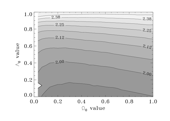
Figure 5: $\left\langle\kappa_{(\theta)}\kappa_{\mathrm{\textsc{\tiny gal}}(\theta_{\mathrm{\textsc{\tiny gal}}})}\right\rangle/\left\langle\kappa_{\mathrm{\textsc{\tiny gal}}(\theta_{\mathrm{\textsc{\tiny gal}}})}^{2}\right\rangle$ for a CDM model consistent with the values of ($\Omega_{0},\Lambda)$. $\theta=\theta_{\mathrm{\textsc{\tiny gal}}}=2^{\prime}$.

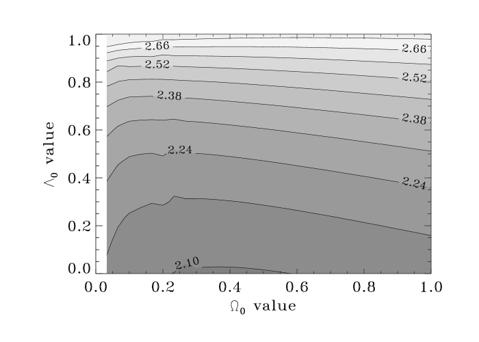
Figure 6: $\left\langle\vec{\nabla}\kappa_{(\theta)}\cdot\vec{\nabla}\kappa_{\mathrm{\textsc{\tiny gal}}(\theta_{\mathrm{\textsc{\tiny gal}}})}\right\rangle/\left\langle(\vec{\nabla}\kappa_{\mathrm{\textsc{\tiny gal}}(\theta_{\mathrm{\textsc{\tiny gal}}})})^{2}\right\rangle$ for a CDM model. $\theta=\theta_{\mathrm{\textsc{\tiny gal}}}=2^{\prime}$.

III.5 Cosmic variance

In previous sections we looked at the sensitivity of observable quantities which mixed galaxy weak lensing surveys and CMB polarization detection. It is very unlikely that both surveys will be able to cover, with a good resolution and low foreground contamination, a large fraction of the sky. It seems however reasonable to expect to have at our disposal patches of at least a few hundreds square degrees. The issue we address in this section is to estimate the cosmic variance of such a detection in joint surveys in about 100 square degrees.

The computation of cosmic variance is a classical problem in cosmological observation [20]. A natural estimate for an ensemble average $\left\langle X\right\rangle$ is its geometrical average. If the survey has size $\Sigma$ then,

$$\overline{X}=\frac{1}{\Sigma}\int_{\Sigma}{\mathrm{d}}^{2}\alpha\,X(\vec{\alpha})$$ (55)

For a compact survey with circular shape of radius $\Xi$ we formally have,

$$\overline{X}=\int\frac{{\mathrm{d}}^{2}k}{2\pi}\,\,\widetilde{X}(\vec{k})\,W(k\,\Xi).$$ (56)

For sake of simplicity this is what we use in the following but we will see that the shape of the survey has no significant consequences.

Taking $\overline{X}$ as an estimate of $\langle X\rangle$ (the ensemble average of $X$), leads to an error of the order $\sqrt{\left\langle\overline{X}^{2}\right\rangle-\left\langle\overline{X}\right\rangle^{2}}$which usually scales like $1/\sqrt{\Sigma}$ if the survey is large enough.

When we are measuring ${\cal X}_{\natural}$ on a small patch of the sky, we are apart from the statistical value by the same kind of error. We can neglect the errors on $\left\langle\Delta\hat{E}^{2}\right\rangle$, $\left\langle(\nabla\hat{E})^{2}\right\rangle$, $\left\langle(\nabla\kappa_{\mathrm{\textsc{\tiny gal}}})^{2}\right\rangle$and $\left\langle\kappa_{\mathrm{\textsc{\tiny gal}}}^{2}\right\rangle$; those may not be the dominant source of discrepancy and can even be measured on wider and independent samples. The biggest source of error is the measure of $\left\langle\Delta\hat{B}b_{\natural}\right\rangle$. It is given by,

$$C_{\natural}=\sqrt{\left\langle\left(\overline{\Delta\hat{B}b_{\natural}}-{\overline{\Delta\hat{B}}}\,{\overline{b_{\natural}}}\right)^{2}\right\rangle-\left\langle\overline{\Delta\hat{B}b_{\natural}}-{\overline{\Delta\hat{B}}}\,{\overline{b_{\natural}}}\right\rangle^{2}}.$$ (57)

The computation of (57) is made easier if we write explicitly the geometrical average as a summation over $N$ measurement points ($N$ can be as large as we want),

$$\overline{X}=\frac{1}{N}\sum^{N}_{i=1}X(\theta_{i}),$$ (58)

we then developed (57), and replace the ensemble average of the summation sign by the geometrical average over the survey size. We are left with a sum of correlators containing $8$ fields taken at 2, 3 and 4 different points. The calculations can be carried out analytically if we assume that all our fields follow Gaussian statistics, which is reasonable at the scale we are working on. In that case indeed, we can take advantage of the Wick theorem to contract each of the $8$ fields correlators in products of $2$ points correlation functions. By definition, (57) contains only connected correlators, moreover the ensemble averages $\langle\Delta\hat{B}\rangle$ and $\langle b_{\natural}\rangle$ vanish, therefore only a small fraction of correlators among all the possible combination of the $8$ fields survive. We can use a simple diagrammatic representations to describe their geometrical shape. All the non vanishing terms in $C_{\natural}$ are given in Fig. 7. Each line between two vertex represents a $2$ points correlation function such as $\langle X(\vec{\alpha}_{1})X(\vec{\alpha}_{2})\rangle$, and the different symbols at the vertex correspond to different $X$ fields (the cross stands for $\Delta P$, the dot for $\gamma_{\mathrm{\textsc{\tiny cmb}}}$, and the open dot stands for $\gamma_{\mathrm{\textsc{\tiny gal}}}$). The $\mathcal{A}$-terms represent terms where the two top (and the two bottom) $\Delta B$ and $b_{\natural}$ are taken at the same point, but top and bottom fields are not at the same place. The $\mathcal{B}$-terms are three points diagrams: the top $\Delta B$ and $b_{\natural}$ are at the same point whereas the right and left bottom vertexes are at two different locations. The $\mathcal{C}$ terms are four-points diagrams, where each vertex is at a different point. To illustrate our notations, let us write ${\mathcal{B}}^{\natural}_{2c}$ as an example,

$$\begin{array}[]{ccc}{\mathcal{B}}^{\natural}_{2c}&=&\langle\gamma_{\mathrm{\textsc{\tiny cmb}}}(\vec{\alpha}_{1})\gamma_{\mathrm{\textsc{\tiny gal}}}(\vec{\alpha}_{2})\rangle\langle\gamma_{\mathrm{\textsc{\tiny gal}}}(\vec{\alpha}_{3})\gamma_{\mathrm{\textsc{\tiny cmb}}}(\vec{\alpha}_{1})\rangle\times\\ &&\langle\Delta P(\vec{\alpha}_{1})\Delta P(\vec{\alpha}_{1})\rangle\langle\Delta P(\vec{\alpha}_{2})\Delta P(\vec{\alpha}_{3})\rangle\end{array}$$

$$C_{\natural} = \framebox{$2\times\underbrace{\parbox{39.83385pt}{\vspace{2mm}\hskip 2.84526pt\diagrm\char 1\relax\vspace{2mm}}}_{{\mathcal{A}}^{\natural}_{1}}+\underbrace{\parbox{39.83385pt}{\vspace{2mm}\hskip 2.84526pt\diagrm\char 2\relax\vspace{2mm}}}_{{\mathcal{A}}_{2n}^{\natural}}+\underbrace{\parbox{39.83385pt}{\vspace{2mm}\hskip 2.84526pt\diagrm\char 3\relax\vspace{2mm}}}_{{\mathcal{A}}^{\natural}_{2c}}$}$$

$$+2\times\underbrace{\parbox{39.83385pt}{\vspace{2mm}\hskip 2.84526pt\diagrm\char 4\relax\vspace{2mm}}}_{{\mathcal{A}}_{3n}^{\natural}}+2\times\underbrace{\parbox{39.83385pt}{\vspace{2mm}\hskip 2.84526pt\diagrm\char 5\relax\vspace{2mm}}}{\mathcal{A}}_{3c}^{\natural}$$

$$-2\times\underbrace{\parbox{39.83385pt}{\vspace{2mm}\hskip 2.84526pt\diagrm\char 6\relax\vspace{2mm}}}_{{\mathcal{B}}_{1}^{\natural}}+\underbrace{\parbox{39.83385pt}{\vspace{2mm}\hskip 2.84526pt\diagrm\char 7\relax\vspace{2mm}}}_{{\mathcal{B}}_{2n}^{\natural}}+\underbrace{\parbox{39.83385pt}{\vspace{2mm}\hskip 2.84526pt\diagrm\char 8\relax\vspace{2mm}}}_{{\mathcal{B}}_{2c}^{\natural}}$$

$$+2\times\underbrace{\parbox{39.83385pt}{\vspace{2mm}\hskip 2.84526pt\diagrm\char 9\relax\vspace{2mm}}}_{{\mathcal{B}}_{3n}^{\natural}}+2\times\underbrace{\parbox{39.83385pt}{\vspace{2mm}\hskip 2.84526pt\diagrm\char 10\relax\vspace{2mm}}}_{{\mathcal{B}}_{3c}^{\natural}}$$

$$+2\times\underbrace{\parbox{39.83385pt}{\vspace{2mm}\hskip 2.84526pt\diagrm\char 11\relax\vspace{2mm}}}_{{\mathcal{C}}_{n}^{\natural}}+4\times\underbrace{\parbox{39.83385pt}{\vspace{2mm}\hskip 2.84526pt\diagrm\char 12\relax\vspace{2mm}}}_{{\mathcal{C}}_{c}^{\natural}}$$

Figure 7: Diagrammatic representation of the terms contributing to the cosmic variance of the correlation coefficients. In this representation the vertex      ‚    represents $\Delta\hat{B}$; the cross stands for the $\Delta P$ part, the dot for $\gamma_{\mathrm{\textsc{\tiny cmb}}}$. The other vertex      ‹    represents any $b_{\natural}$; the open dot stands for $\gamma_{\mathrm{\textsc{\tiny gal}}}.$ The solid lines connect $\Delta P$ terms and the dashed ones the $\gamma$-s

We only focus on the calculation of the $\mathcal{A}$ terms because we can use the approximation that

$${\mathcal{A}}\gg{\mathcal{B}}\gg{\mathcal{C}}.$$ (59)

Indeed, in perturbative theory, if the survey is large enough, the $n$-points correlation functions naturally dominates over the $n+1$-points correlation function. This is true as long as the local variance is much bigger than the autocorrelation at survey scale and we assume the surveys are still large enough to be in this case.

The general expression for any $\mathcal{A}$ diagram is

$${\mathcal{A}}^{\natural}_{i} = 4\int^{\mathrm{\textsc{\tiny cmb}}}{\cal D}(\chi_{\mathrm{\textsc{\tiny cmb}}1},\vec{l}_{\mathrm{\textsc{\tiny cmb}}1},\vec{k}_{\mathrm{\textsc{\tiny cmb}}1})\,{\cal D}(\chi_{\mathrm{\textsc{\tiny cmb}}2},\vec{l}_{\mathrm{\textsc{\tiny cmb}}2},\vec{k}_{\mathrm{\textsc{\tiny cmb}}2})$$

$$\times\int^{\mathrm{\textsc{\tiny gal}}}{\cal D}(\chi_{\mathrm{\textsc{\tiny gal}}1},\vec{l}_{\mathrm{\textsc{\tiny gal}}1},\vec{k}_{\mathrm{\textsc{\tiny gal}}1})\,{\cal D}(\chi_{\mathrm{\textsc{\tiny gal}}2},\vec{l}_{\mathrm{\textsc{\tiny gal}}2},\vec{k}_{\mathrm{\textsc{\tiny gal}}2})$$

$$\times{\mathcal{G}}^{\rm Ker}_{\natural}(\vec{l}_{\mathrm{\textsc{\tiny cmb}}1},\vec{k}_{\mathrm{\textsc{\tiny cmb}}1_{\bot}})\,{\mathcal{G}}^{\rm Ker}_{\natural}(\vec{l}_{\mathrm{\textsc{\tiny cmb}}2},\vec{k}_{\mathrm{\textsc{\tiny cmb}}2_{\bot}})$$

$$\times{\mathcal{G}}^{\rm Ker}_{\natural}(\vec{l}_{\mathrm{\textsc{\tiny gal}}1},\vec{k}_{\mathrm{\textsc{\tiny gal}}1_{\bot}})\,{\mathcal{G}}^{\rm Ker}_{\natural}(\vec{l}_{\mathrm{\textsc{\tiny gal}}2},\vec{k}_{\mathrm{\textsc{\tiny gal}}2_{\bot}})\,{{\mathcal{M}}}_{i}\left\langle\vec{k}_{i}\mid\vec{l}_{j}\right\rangle$$

$$\times W(|\vec{k}_{\mathrm{\textsc{\tiny cmb}}1_{\perp}}{\mathrm{D}}+\vec{l}_{\mathrm{\textsc{\tiny cmb}}1}|\theta)\,\,W(|\vec{k}_{\mathrm{\textsc{\tiny cmb}}2_{\perp}}{\mathrm{D}}+\vec{l}_{\mathrm{\textsc{\tiny cmb}}2}|\theta)$$

$$\times W(k_{\mathrm{\textsc{\tiny gal}}1_{\perp}}{\mathrm{D}_{1}}\theta_{\mathrm{\textsc{\tiny gal}}})W(l_{\mathrm{\textsc{\tiny gal}}1}\theta)\,\,W(k_{\mathrm{\textsc{\tiny gal}}2_{\perp}}{\mathrm{D}_{2}}\theta_{\mathrm{\textsc{\tiny gal}}})W(l_{\mathrm{\textsc{\tiny gal}}2}\theta)$$

$$\times W\left(|\vec{k}_{\mathrm{\textsc{\tiny gal}}1_{\perp}}{\mathrm{D}_{1}}+\vec{l}_{\mathrm{\textsc{\tiny gal}}1}+\vec{k}_{\mathrm{\textsc{\tiny cmb}}1_{\perp}}{\mathrm{D}_{1}}+\vec{l}_{\mathrm{\textsc{\tiny cmb}}1}|\Xi\right)$$

$$\times W\left(|\vec{k}_{\mathrm{\textsc{\tiny gal}}2_{\perp}}{\mathrm{D}_{2}}+\vec{l}_{\mathrm{\textsc{\tiny gal}}2}+\vec{k}_{\mathrm{\textsc{\tiny cmb}}2_{\perp}}{\mathrm{D}_{2}}+\vec{l}_{\mathrm{\textsc{\tiny cmb}}2}|\Xi\right)$$

where ${\mathcal{M}}_{i}$ gives the 2-point correlations associated with the lines of the diagram. For example :

$${\mathcal{M}}_{1} = \!\!\left\langle\delta(\vec{k}_{\mathrm{\textsc{\tiny gal}}1})\delta(\vec{k}_{\mathrm{\textsc{\tiny cmb}}1})\right\rangle\left\langle\delta(\vec{k}_{\mathrm{\textsc{\tiny gal}}2})\delta(\vec{k}_{\mathrm{\textsc{\tiny cmb}}2})\right\rangle$$ (61)

$$\!\!\!\!\times\left\langle\tilde{E}(l_{\mathrm{\textsc{\tiny gal}}1})\tilde{E}(l_{\mathrm{\textsc{\tiny gal}}2})\right\rangle\left\langle\tilde{E}(l_{\mathrm{\textsc{\tiny cmb}}1})\tilde{E}(l_{\mathrm{\textsc{\tiny cmb}}2})\right\rangle$$

We explicit in the following the computation of ${\mathcal{A}}^{\natural}_{1}$. The other terms follow the same treatment or can be neglected. The lines in the ${\mathcal{A}}^{\natural}_{1}$ diagram give us the relations

$$\vec{k}_{\mathrm{\textsc{\tiny cmb}}1} = -\vec{k}_{\mathrm{\textsc{\tiny gal}}1}=\vec{k}_{1}$$

$$\vec{k}_{\mathrm{\textsc{\tiny cmb}}2} = -\vec{k}_{\mathrm{\textsc{\tiny gal}}2}=\vec{k}_{2}$$ (62)

$$\vec{l}_{\mathrm{\textsc{\tiny cmb}}1} = -\vec{l}_{\mathrm{\textsc{\tiny cmb}}2}=\vec{l}_{\mathrm{\textsc{\tiny cmb}}}$$

$$\vec{l}_{\mathrm{\textsc{\tiny gal}}1} = -\vec{l}_{\mathrm{\textsc{\tiny gal}}2}=\vec{l}_{\mathrm{\textsc{\tiny gal}}}$$

Then, using these relations and the small angular approximation, we have :

$${\mathcal{A}}^{\natural}_{1} = 4\int^{\mathrm{\textsc{\tiny gal}}}{\mathrm{d}}\chi_{1}{\mathrm{d}}\chi_{2}\,{w}_{\mathrm{\textsc{\tiny cmb}}1}{w}_{\mathrm{\textsc{\tiny gal}}1}{w}_{\mathrm{\textsc{\tiny cmb}}2}{w}_{\mathrm{\textsc{\tiny gal}}2}$$

$$\times\int\frac{{\mathrm{d}}^{2}k_{1}{\mathrm{d}}^{2}k_{2}}{(2\pi)^{4}}\frac{{\mathrm{d}}^{2}l_{\mathrm{\textsc{\tiny gal}}}{\mathrm{d}}^{2}l_{\mathrm{\textsc{\tiny cmb}}}}{(2\pi)^{4}}$$

$$\times C_{E}(l_{\mathrm{\textsc{\tiny gal}}})C_{E}(l_{\mathrm{\textsc{\tiny cmb}}})P(k_{1})P(k_{2})$$

$$\times{\mathcal{G}}^{\rm Ker}_{\natural}(\vec{l}_{\mathrm{\textsc{\tiny cmb}}},\vec{k}_{1}){\mathcal{G}}^{\rm Ker}_{\natural}(-\!\vec{l}_{\mathrm{\textsc{\tiny cmb}}},\vec{k}_{2})$$

$$\times{\mathcal{G}}^{\rm Ker}_{\natural}(\vec{l}_{\mathrm{\textsc{\tiny gal}}},-\!\vec{k}_{1}){\mathcal{G}}^{\rm Ker}_{\natural}(-\!\vec{l}_{\mathrm{\textsc{\tiny gal}}},-\!\vec{k}_{2})$$

$$\times W(|\vec{k}_{1}{\mathrm{D}}+\vec{l}_{\mathrm{\textsc{\tiny cmb}}}|\theta)W(|\vec{k}_{2}{\mathrm{D}}+\vec{l}_{\mathrm{\textsc{\tiny cmb}}}|\theta)$$

$$\times W(k_{1}{\mathrm{D}}\theta_{\mathrm{\textsc{\tiny gal}}})W(k_{2}{\mathrm{D}}\theta_{\mathrm{\textsc{\tiny gal}}})W^{2}(l_{\mathrm{\textsc{\tiny gal}}}\theta)$$

$$\times W^{2}(|\vec{l}_{\mathrm{\textsc{\tiny gal}}}+\vec{l}_{\mathrm{\textsc{\tiny cmb}}}|\Xi).$$

We apply the decomposition of $W_{1}\left(|\vec{k}{\mathrm{D}}(\chi)+\vec{l}|\theta\right)$ we used in eq. (48). The geometry of our problem is the same and the result (49) still holds for the terms in $W_{1}\left(|\vec{k}_{1}{\mathrm{D}}(\chi_{1})+\vec{l}_{\mathrm{\textsc{\tiny cmb}}}|\theta\right)$ and $W_{1}\left(|\vec{k}_{2}{\mathrm{D}}(\chi_{2})+\vec{l}_{\mathrm{\textsc{\tiny cmb}}}|\theta\right)$. This however is not true for $W_{1}^{2}\left(|\vec{l}_{\mathrm{\textsc{\tiny gal}}}+\vec{l}_{\mathrm{\textsc{\tiny cmb}}}|\Xi\right)$ for which the application of the re-summation theorem does not bring any simplification. Then, neglecting all the $W_{3}$ parts and after integration on the $\phi_{k_{i}}$, for the ${\tiny\Delta}$-term, we have,

$${\mathcal{A}}_{1}^{{\tiny\Delta}} = \int^{\mathrm{\textsc{\tiny gal}}}{\mathrm{d}}\chi_{1}{\mathrm{d}}\chi_{2}\,{w}_{\mathrm{\textsc{\tiny cmb}}1}{w}_{\mathrm{\textsc{\tiny gal}}1}{w}_{\mathrm{\textsc{\tiny cmb}}2}{w}_{\mathrm{\textsc{\tiny gal}}2}$$

$$\times\int\frac{{\mathrm{d}}k_{1}{\mathrm{d}}k_{2}}{(2\pi)^{2}}\frac{{\mathrm{d}}^{2}l_{\mathrm{\textsc{\tiny gal}}}{\mathrm{d}}^{2}l_{\mathrm{\textsc{\tiny cmb}}}}{(2\pi)^{4}}\>\,{l_{\mathrm{\textsc{\tiny gal}}}^{4}l_{\mathrm{\textsc{\tiny cmb}}}^{4}}\>k_{1}k_{2}$$

$$\times C_{E}(l_{\mathrm{\textsc{\tiny gal}}})C_{E}(l_{\mathrm{\textsc{\tiny cmb}}})P(k_{1})P(k_{2})$$

$$\times W^{2}(|\vec{l}_{\mathrm{\textsc{\tiny gal}}}+\vec{l}_{\mathrm{\textsc{\tiny cmb}}}|\Xi)\cos^{2}2\left(\phi_{l_{\mathrm{\textsc{\tiny cmb}}}}-\phi_{l_{\mathrm{\textsc{\tiny gal}}}}\right)$$

$$\times W(k_{1}{\mathrm{D}}\theta_{\mathrm{\textsc{\tiny gal}}})W(k_{2}{\mathrm{D}}\theta_{\mathrm{\textsc{\tiny gal}}})W^{2}(l_{\mathrm{\textsc{\tiny gal}}}\theta)$$

$$\times W(k_{1}{\mathrm{D}}\theta)W(k_{2}{\mathrm{D}}\theta)W^{2}(l_{\mathrm{\textsc{\tiny cmb}}}\theta).$$

Note that for the evaluation of the ${\tiny\nabla}$ part, using the same kind of method, we obtain the same equation as eq. (III.5) where ${l_{\mathrm{\textsc{\tiny gal}}}^{4}l_{\mathrm{\textsc{\tiny cmb}}}^{4}}$ is replaced by ${l_{\mathrm{\textsc{\tiny gal}}}^{2}l_{\mathrm{\textsc{\tiny cmb}}}^{2}k_{1}^{2}k_{2}^{2}}/2$.

We can get rid of the remaining $W^{2}\!\left(|\vec{l}_{\mathrm{\textsc{\tiny gal}}}+\vec{l}_{\mathrm{\textsc{\tiny cmb}}}|\Xi\right)$ with another approximation. The power spectrum $C_{E}(l)$ favors large values of $l$ whereas $W^{2}(|\vec{l}_{\mathrm{\textsc{\tiny gal}}}+\vec{l}_{\mathrm{\textsc{\tiny cmb}}}|\Xi)$ will be non-zero for $|\vec{l}_{\mathrm{\textsc{\tiny gal}}}+\vec{l}_{\mathrm{\textsc{\tiny cmb}}}|\sim{1/\Xi}$. Then for typical survey size of about one hundred square-degrees, $|\vec{l}_{\mathrm{\textsc{\tiny gal}}}+\vec{l}_{\mathrm{\textsc{\tiny cmb}}}|\ll l_{i}$ and we can assume $\vec{l}_{\mathrm{\textsc{\tiny gal}}}\sim-\vec{l}_{\mathrm{\textsc{\tiny cmb}}}$ and $\vec{l}_{\mathrm{\textsc{\tiny gal}}}+\vec{l}_{\mathrm{\textsc{\tiny cmb}}}=\vec{\epsilon}$. In this limit, $\cos^{2}2\left(\phi_{l_{\mathrm{\textsc{\tiny cmb}}}}-\phi_{l_{\mathrm{\textsc{\tiny gal}}}}\right)=1$ and ${\mathcal{A}}^{\natural}_{1}$ can be written

$${\mathcal{A}}^{{\tiny\Delta}}_{1} = \int\frac{l\,{\mathrm{d}}l}{(2\pi)^{2}}\,{l^{8}}C_{E}^{2}(l)W^{4}(l\theta)\,\int\frac{{\mathrm{d}}^{2}\epsilon}{2\pi}\,{l^{8}}W_{1}^{2}(\epsilon\,\,\Xi)$$

$$\times\left[\int^{\mathrm{\textsc{\tiny gal}}}\!\!{\mathrm{d}}\chi{w}_{\mathrm{\textsc{\tiny cmb}}}{w}_{\mathrm{\textsc{\tiny gal}}}\int\frac{k\,{\mathrm{d}}k}{2\pi}\,P(k)\,W(k{\mathrm{D}}\theta)\,W(k{\mathrm{D}}\theta_{\mathrm{\textsc{\tiny gal}}})\right]^{2}$$

which is essentially the cosmic variance of $\left\langle\Delta E^{2}\right\rangle$, for the ${\tiny\Delta}$ part and of $\left\langle(\nabla E)^{2}\right\rangle$ for the ${\tiny\nabla}$ one (where $l^{8}$ in eq. (III.5) is replaced by $l^{4}k_{1}^{2}k_{2}^{2}/2$). Finally we have,

$$\!\!\!\!\!\!\!\!\frac{{\mathcal{A}}^{{\tiny\Delta}}_{1}}{\left\langle B_{(\theta)}b_{{\tiny\Delta}(\theta,\theta_{\mathrm{\textsc{\tiny gal}}})}\right\rangle^{2}} = \frac{2\pi}{\Sigma}\frac{\int{\mathrm{d}}l\,l^{9}C_{E}^{2}(l)W_{1}^{4}(l\,\theta)}{\left(\int{\mathrm{d}}l\,l^{5}C_{E}(l)W_{1}^{2}(l\,\theta)\right)^{2}}$$

$$\propto \textrm{Cosmic variance of }\Delta E^{2}$$

where $\Sigma=\pi\Xi^{2}$ in case of a disc shape survey. We show in Fig. 8 numerical results for a $100\,\mathrm{deg}^{2}$ survey although the numerical calculations were done with a Gaussian window function instead of a top-hat.

Figure 8: Comparison between $\sqrt{2\,A_{1}^{{\tiny\Delta}}/\mathrm{signal}_{{\tiny\Delta}}}$ (solid line) and $\sqrt{2\,A_{1}^{{\tiny\nabla}}/\mathrm{signal}_{{\tiny\nabla}}}$ (dashed line). The $C_{\ell}$ are from a $\Omega=0.3$, $\Lambda=0.7$ model. The survey size is $100\,\mathrm{deg}^{2}$, and Gaussian filters were used.

Numerically, for $\theta=10^{\prime}$, we get

$$\frac{{\mathcal{A}}^{\natural}_{1}}{\left\langle B_{(\theta)}b_{\natural(\theta,\theta_{\mathrm{\textsc{\tiny gal}}})}\right\rangle^{2}}\sim\frac{(3.7\%)^{2}}{\Sigma/100\textrm{ deg}^{2}}.$$ (67)

We expect that for the same reasons, the ${\mathcal{A}}^{\natural}_{2}$ terms will be dominated by the weak lensing variance. Yet a correct evaluation here is harder to reach. We have made this estimation within the framework of a power law $P(k)$. With this simplification in hand, we can write for ${\mathcal{A}}_{2n}^{\natural}$ (we focus only the ${\tiny\Delta}$ part, but the same discussion holds for the ${\tiny\nabla}$ observable.)

$$\frac{{\mathcal{A}}_{2n}^{{\tiny\Delta}}}{\left\langle B_{(\theta)}b_{{\tiny\Delta}(\theta,\theta_{\mathrm{\textsc{\tiny gal}}})}\right\rangle^{2}} =$$

$$\frac{1}{r^{2}}\int{\mathrm{d}}^{2}k_{1}{\mathrm{d}}^{2}k_{2}\,P(k_{1})P(k_{2})\cos^{2}\left(\phi_{k_{1}}-\phi_{k_{2}}\right)$$

$$\times\frac{W_{1}^{2}(k_{1}\theta)W_{1}^{2}(k_{2}\theta_{\mathrm{\textsc{\tiny gal}}})W_{1}^{2}(|\vec{k}_{1}+\vec{k}_{2}|\Xi)}{\left[\int{\mathrm{d}}^{2}k\,P(k)W_{1}(k\theta)W_{1}(k\theta_{\mathrm{\textsc{\tiny gal}}})\right]^{2}}.$$

The last integral behaves essentially like the cosmic variance of $\left\langle\kappa^{2}\right\rangle$. More exactly, it goes like $1/\sqrt{2}$ this variance. It should even be smaller, because of the extra $\cos^{2}$ factor. We evaluated this cosmic variance using the ray-tracing simulations described in [24]. These simulations provide us with realistic convergence maps (for the cosmological models we are interested in) with a resolution of 0.1’, and a survey size of 9 square degrees. The sources have been put at a redshift unity, and the ray-lights are propagated through a simulated Universe whose the density field has been evolved from an initial CDM power spectrum. The measured cosmic variance of $\langle\kappa_{(\theta)}\kappa_{(\theta_{\mathrm{\textsc{\tiny gal}}})}\rangle$ is about $3\%$ (see Table 2) when filtered at scales $\theta_{\mathrm{\textsc{\tiny gal}}}=5^{\prime}$ and $\theta=10^{\prime}$ for a $\Omega_{0}=0.3$ cosmology.

	${\mathrm{C}osVar}\left(\left\langle\kappa^{2}\right\rangle\right)$		${\mathrm{C}osVar}\left(\left\langle(\vec{\nabla}\kappa)^{2}\right\rangle\right)$
	$\Omega_{0}=0.3$	$\Omega_{0}=1$	$\Omega_{0}=0.3$	$\Omega_{0}=1$
$\theta=5^{\prime},\,\theta_{\mathrm{\textsc{\tiny gal}}}=2.5^{\prime}$	2.94%	1.86%	2.88%	2.07%
$\theta=5^{\prime},\,\theta_{\mathrm{\textsc{\tiny gal}}}=5^{\prime}$	3.02%	1.87%	2.23%	1.75%
$\theta=10^{\prime},\,\theta_{\mathrm{\textsc{\tiny gal}}}=5^{\prime}$	3.54%	2.03%	4.25%	3.02%

Table 2: Values of the cosmic variance of $\left\langle\kappa^{2}\right\rangle$ and $\left\langle(\vec{\nabla}\kappa)^{2}\right\rangle$ for different models and different filtering radius. The size of the survey is $100\,\textrm{deg}^{2}$. For the $\Omega_{0}=0.3$ ($\Omega_{0}=1$) model, we use 5 (7) independent ray-tracing realizations (see [24]) to estimate the cosmic variance in a $9\,$deg² survey, which is then rescaled to the cosmic variance we should obtain for a $100\,$deg² survey. Given the low number of realizations, the values here can only be used as a good estimation of the order of magnitude of ${\mathrm{C}osVar}\left(\left\langle\kappa^{2}\right\rangle\right)$ and ${\mathrm{C}osVar}\left(\left\langle(\vec{\nabla}\kappa)^{2}\right\rangle\right)$. It also seems, from these figures that the cosmic variance of $\left\langle(\vec{\nabla}\kappa)^{2}\right\rangle$ is more degraded by the difference in filtering beams than the other.

An estimation of ${\mathcal{A}}^{{\tiny\Delta}}_{2n}$ is then given by,

$$\frac{{\mathcal{A}}^{{\tiny\Delta}}_{2n}}{\left\langle B_{(\theta)}b_{{\tiny\Delta}(\theta,\theta_{\mathrm{\textsc{\tiny gal}}})}\right\rangle^{2}}\sim\left(\frac{2.12\%}{r}\right)^{2}\frac{1}{\Sigma/100\textrm{ deg}^{2}}.$$ (70)

Since $r_{{\tiny\nabla}}$ is very comparable to $r$, we very roughly estimate ${\mathcal{A}}^{{\tiny\nabla}}_{2n}$

$$\frac{{\mathcal{A}}^{{\tiny\nabla}}_{2n}}{\left\langle B_{(\theta)}b_{{\tiny\nabla}(\theta,\theta_{\mathrm{\textsc{\tiny gal}}})}\right\rangle^{2}}\sim\left(\frac{2.12\%}{r}\right)^{2}\frac{1}{\Sigma/100\textrm{ deg}^{2}}.$$ (71)

The same considerations gives

$$\frac{{\mathcal{A}}^{\natural}_{2n}}{\left\langle B_{(\theta)}b_{\natural(\theta,\theta_{\mathrm{\textsc{\tiny gal}}})}\right\rangle^{2}} = \frac{(2.12\%)^{2}}{\Sigma/100\textrm{ deg}^{2}}.$$ (72)

There is no $r$ dependency here; the diagram cross-correlates $\kappa_{\mathrm{\textsc{\tiny cmb}}}$ and $\kappa_{\mathrm{\textsc{\tiny gal}}}$.

We can approximate the remaining $\mathcal{A}$-terms. They should be smaller than the former. We have

$${\mathcal{A}}^{\natural}_{3n} \sim \frac{1}{r_{\natural}^{2}}\frac{(2.12\%\times 3.7\%)^{2}}{\Sigma/100\textrm{ deg}^{2}}\left\langle B_{(\theta)}b_{\natural(\theta,\theta_{\mathrm{\textsc{\tiny gal}}})}\right\rangle^{2}$$

$$\ll {\mathcal{A}}^{\natural}_{2n}$$

and

$${\mathcal{A}}^{\natural}_{3c} \sim \frac{(2.12\%\times 3.7\%)^{2}}{\Sigma/100\textrm{ deg}^{2}}\left\langle B_{(\theta)}b_{\natural(\theta,\theta_{\mathrm{\textsc{\tiny gal}}})}\right\rangle^{2}$$

$$\ll {\mathcal{A}}^{\natural}_{2c}.$$

Then, only the ${\mathcal{A}}^{\natural}_{1}$ and ${\mathcal{A}}^{\natural}_{2}$ terms (boxed on Fig. 7) contribute substantially to the cosmic variance of ${\cal X}_{\natural}$. Since ${\mathcal{A}}^{\natural}_{1}$ and ${\mathcal{A}}^{\natural}_{2}$ are respectively the cosmic variance of $\left\langle\Delta E^{2}\right\rangle$ (resp. $\left\langle(\vec{\nabla}E)^{2}\right\rangle)$ and of $\left\langle\kappa^{2}\right\rangle$ (resp. $\left\langle(\vec{\nabla}\kappa)^{2}\right\rangle$), we can write the variance of ${\cal X}_{\natural}$ as

$${\mathrm{C}osVar}({\cal X}_{{\tiny\Delta}}) =$$

$${\mathrm{C}osVar}\left(\left\langle\Delta E^{2}\right\rangle\right)+\left(\frac{1+r^{2}}{2\,r^{2}}\right){\mathrm{C}osVar}\left(\left\langle\kappa^{2}\right\rangle\right).$$

and

$${\mathrm{C}osVar}({\cal X}_{{\tiny\nabla}}) =$$

$${\mathrm{C}osVar}\left(\left\langle(\vec{\nabla}E)^{2}\right\rangle\right)+\left(\frac{1+r_{{\tiny\nabla}}^{2}}{2\,r_{{\tiny\nabla}}^{2}}\right){\mathrm{C}osVar}\left(\left\langle(\vec{\nabla}\kappa)^{2}\right\rangle\right).$$

Table 3 presents numerical results for various filtering scenarii and models.

	${\mathrm{C}osVar}\left({\cal X}_{{\tiny\Delta}}\right)$		${\mathrm{C}osVar}\left({\cal X}_{{\tiny\nabla}}\right)$
	$\Omega_{0}=0.3$	$\Omega_{0}=1$	$\Omega_{0}=0.3$	$\Omega_{0}=1$
$\theta=5^{\prime},\,\theta_{\mathrm{\textsc{\tiny gal}}}=2.5^{\prime}$	6.44%	4.77%	6.06%	4.72%
$\theta=5^{\prime},\,\theta_{\mathrm{\textsc{\tiny gal}}}=5^{\prime}$	6.58%	4.79%	4.99%	4.23%
$\theta=10^{\prime},\,\theta_{\mathrm{\textsc{\tiny gal}}}=5^{\prime}$	8.71%	6.73%	9.49%	7.62%

Table 3: Values of the cosmic variance of ${\cal X}_{\natural}$. The survey size is $100\,\textrm{deg}^{2}$. We used the results presented in Table2 and Fig. 8. The $r_{\natural}$ parameters are assumed to be equal and set to 0.4. We didn’t take into account the filtering effects in the definition of $r$. The difference due to filtering correction is small, though. From this estimations, we can expect a cosmic variance for ${\cal X}_{\natural}$of less than 10% for realistic scenarii.

The two quantities, $b_{{\tiny\Delta}}$ and $b_{{\tiny\nabla}}$, lead to similar cosmic variance that are rather small. Obviously it would be even better to use $b=b_{{\tiny\Delta}}+b_{{\tiny\nabla}}$. For such a quantity the resulting cosmic variance for the cross-correlation coefficient should even be smaller, by a factor $\sqrt{2}$, although a detailed analysis is made complicated because of the complex correlation patterns it contains.

IV Conclusion

We have computed a first order mapping that describes, in real space, the weak lensing effects on the CMB polarization. In particular we derived the explicit mathematical relation between the primary CMB polarization and the shear field at leading order in lens effect. It demonstrates that a $B$-component of the polarization field can be induced by lens couplings. We have shown however that the $B$-map alone cannot lead to a non-ambiguous reconstruction of the projected mass map.

Nonetheless, the $B$-component can potentially exhibit a significant correlation signal with local weak lensing surveys. This opens a new window for detecting lens effects on CMB maps. In particular, and contrary to previous studies involving the temperature maps alone, we found that such a correlation can be measured with a rather high signal to noise ratio even in surveys of rather modest size and resolution. Anticipating data sets that should be available in the near future, ($100\,\textrm{deg}^{2}$ survey, with $5^{\prime}$ resolution for galaxy survey and $10^{\prime}$ Gaussian beam size for CMB polarization detection), we have obtained a cosmic variance around $8\%$. Needless is to say that this estimation does not take into account systematics and possible foreground contaminations. It shows anyway that Cosmic Microwave Background polarization contains a precious window for studying the large scale mass distribution and consequently putting new constraints on the cosmological parameters.

In this paper we have investigated specific quantities that would accessible to observations. They both would permit to put constraint on the cosmological constant. The simulated maps we presented here are only of illustrative interest. We plan to complement this study with extensive numerical experiments to validate our results (in particular on the cosmic variance), and explore the effect of realistic ingredients we did not include in our simple analytical framework, a shear non-gaussianity, lens-lens coupling and so forth.

- [1] Among the current and future high precision observations, the most promising are probably the BOOMERanG balloon experiment (P. de Bernardis et al. astro-ph/9911461); the MAP satellite mission, (C.L. Bennett et al. AAS 187 (1995) 7109) and Planck Surveyor satellite mission (M. Bersanelli et al., COBRAS/SAMBA report on the phase A study, ESA report D/SCI(96)3).
- [2] M. Zaldarriaga, D. Spergel, U. Seljak, ApJ. 488 (1997) 1-13, G. Efstathiou, J. R. Bond MNRAS 304 (1999) 75.
- [3] S. Perlmutter et al., ApJ 517 (1999) 565-586; A. G. Riess et al., Astron.J. 116 (1998) 1009-1038.
- [4] A. Aguirre, ApJ 525 (1999) 583; T. Totani & C. Kobayashi, ApJL 526 (1999) 65; M. Livio, astro-ph/9903264; K. Nomoto, astro-ph/9907386;P. Valageas, astro-ph/9904300.
- [5] Y. Mellier, ARAA 37 (1999) 127.
- [6] A. Blanchard, J. Schneider A&A 184 (1987) 1 ; U. Seljak ApJ 463 (1996) 1 .
- [7] F. Bernardeau, A&A 324 (1997) 15 ; M. Zaldarriaga, astro-ph/9910498.
- [8] F. Bernardeau, A&A 338 (1998) 767.
- [9] U. Seljak, M. Zaldarriaga, Phys.Rev.Lett. 82 (1999) 2636; M. Zaldarriaga, U. Seljak, Phys.Rev. D; J. Guzik, U. Seljak & M. Zaldarriaga, astro-ph/9912505.
- [10] M. Zaldarriaga, U. Seljak, Phys.Rev. D58 (1998) 023003.
- [11] K. Benabed & F. Bernardeau, astro-ph/9906161, Phys. Rev D, in press.
- [12] M. Suginohara, T. Suginohara, D. N. Spergel, ApJ 495 (1998) 511 ; H. V. Peiris & D. N. Spergel, astro-ph/0001393.
- [13] L. Van Waerbeke, F. Bernardeau & K. Benabed, astro-ph/9910366.
- [14] W. Hu, astro-ph/0001303.
- [15] V. Faraoni, Astron.Astrophys. 272 (1993) 385.
- [16] F. Bernardeau, L. Van Waerbeke, Y. Mellier Astronomy and Astrophysics, 322 (1997) 1.
- [17] J.A. Peacock, S.J. Dodds, MNRAS, 280 (1996) L19.
- [18] U. Seljak, ApJ 482 (1997) 6; W. Hu & M. White, New Astronomy 2 (1997) 323; J. Lesgourgues, D. Polarski, S. Prunet, A. A. Starobinsky gr-qc/9906098.
- [19] A. Riazuelo, PhD thesis, University of Paris 11.
- [20] M. Srednicki, ApJL 416 (1993) 1.
- [21] L. Van Waerbeke, F. Bernardeau, Y. Mellier, astro-ph/9807007.
- [22] F. R. Bouchet, S. Prunet & S. K. Sethi MNRAS 302 (1999) 663 ; S. Prunet, S. K. Sethi & F. R. Bouchet astro-ph/9911243.
- [23] W. Hu, astro-ph/9907103.
- [24] B. Jain, U. Seljak, S. White, To appear in ApJ, astro-ph/9901191.