Boltzmann equations for neutrinos with flavor mixings

Abstract

With a view of applications to the simulations of supernova explosion and proto neutron star cooling, we derive the Boltzmann equations for the neutrino transport with the flavor mixing based on the real time formalism of the nonequilibrium field theory and the gradient expansion of the Green function. The relativistic kinematics is properly taken into account. The advection terms are derived in the mean field approximation for the neutrino self-energy whiles the collision terms are obtained in the Born approximation. The resulting equations take the familiar form of the Boltzmann equation with corrections due to the mixing both in the advection part and in the collision part. These corrections are essentially the same as those derived by Sirera et al. for the advection terms and those by Raffelt et al. for the collision terms, respectively, though the formalism employed here is different from theirs. The derived equations will be easily implemented in numerical codes employed in the simulations of supernova explosions and proto neutron star cooling.

I introduction

The neutrino transport plays an important role in some astrophysical phenomena such as supernova explosions and the following proto neutron star cooling (e.g. [1, 2, 3, 4] and references therein). In their studies, the Boltzmann equation or its approximate versions are commonly employed to describe the temporal variations of neutrino distributions in the phase space. These equations are usually derived from the following assumptions[5, 6, 7]: (1) the neutrinos are propagating along the geodesics for a massless particle, $p^{\mu}p_{\mu}=0$, and the volume in the phase space occupied by these neutrinos is not varied along their world line if there is no reaction. (2) the variation of the neutrino population due to reactions is described by the so-called collision terms obtained with the stohszahl ansatz. With the masses non-diagonal in the neutrino flavor space, the neutrino oscillation occurs among different flavors of neutrinos(e.g. [8] and references therein). It is thus interesting from an academic point of view how this oscillation phenomenon is described by the generalized Boltzmann equations[9, 10, 11, 12, 13, 14]. It is also important from a practical point of view for those who are interested in the possible significant consequences the oscillation might give in astrophysical events[15, 16, 17, 18]. In collapse-driven supernova explosions, for example, this is particularly the case if the resonance of oscillation occurs near a neutrino sphere where neutrinos are interacting with other particles and thus the oscillation should be treated simultaneously with these reactions and possibly with the evolution of the matter distribution as well. The purpose of this paper is to provide the formulation which can be easily implemented in those numerical simulations.

In considering the transport equation with the oscillation, we have to rely on a more formal derivation of the Boltzmann equation. This might be done in a couple of ways. Sirera and Pérez[14], for instance, based their derivation on the relativistic Wigner function approach in the mean field approximation. Although they took the relativistic kinematics properly into account, they did not obtain the collision terms, since it is difficult to go beyond the mean field approximation in their formalism. Raffelt et al.[10, 11], on the other hand, obtained their transport equation via the density matrix approach. Although they derived the collision terms, they did not consider the spatially inhomogeneous system. In this paper, we derive the relativistic Boltzmann equation including corrections due to the oscillation both in the advection terms and the collision terms by employing the real time formalism of the nonequilibrium field theory[19, 20, 21]. In this approach, the dispersion relation and the collision terms are derived on the same basis, that is, a particular approximation for the self-energy of neutrinos, which is conveniently represented with Feynman diagrams.

The paper is organized as follows. We first derive a generic form of the transport equation without specifying particular equations of motion of fields. Then, the formulation is applied to the neutrino flavor oscillations. In so doing, we ignore small corrections of the order of $m^{2}_{\nu}/E_{\nu}$ except for the terms responsible for the flavor conversion, as is usually the case. Here $m_{\nu}$ and $E_{\nu}$ are typical mass and energy of neutrinos in the observer’s inertial frame. In this limit, as shown later, the left handed neutrinos are decoupled from the right handed ones and the difference between Majorana mass and Dirac mass never shows up in the flavor mixing. The general relativistic corrections are obtained up to the leading order of $\lambda_{\nu}/R$, where $\lambda_{\nu}$ is a typical wave length of neutrino and $R$ is a scale height of the background matter distribution.

II formulation

A general derivation of transport equations

In this section we derive general transport equations for multi-component fields based on the real time formalism of nonequilibrium field theory by Keldysh[19, 20, 21]. In this formalism, we introduce path-ordered products of operators on the closed time-path, which extends from $t=-\infty$ to $t=+\infty$ then back to $t=-\infty$. In this product, the operator with a time argument which comes later on the above time-path is put to the left of other operators whose time arguments come earlier. Accordingly the path-ordered Green function is defined as

$$i\,G_{pij}(t_{1},t_{2})\ \equiv\ \langle\,T_{p}\ \psi_{i}(t_{1})\ \psi_{j}^{\dagger}(t_{2})\,\rangle\quad.$$ (1)

Here $T_{p}$ stands for the path-ordered product of the following operators. The subscript $ij$ of the Green function denotes the components of the field. The bracket $\langle\cdots\rangle$ represents that arguments are averaged over the ensemble specified by a density operator $\rho$ as $T\!r\{\cdots\rho\}$, where $T\!r$ is a trace operator. We define a generating functional of the Green function as

$$Z(J,J^{\dagger})\ \equiv\ T\!r\left\{T_{p}\,\left[\exp\left(i\,\sum_{i}\int_{p}\!d^{4}\!x\ \left(\,J^{\dagger}_{i}(x)\psi_{i}(x)\ +\ J_{i}(x)\psi^{\dagger}_{i}(x)\right)\right)\right]\,\rho\right\}\ \equiv\ \exp\left[\,i\,W(J,J^{\dagger})\,\right]\quad.$$ (2)

The Green function is obtained by the functional derivative, $i\,G_{pij}(x,y)\,=\,\frac{\delta\ \ \ }{i\,\delta\!J^{\dagger}_{i}(x)}\frac{\delta\ \ \ }{i\,\delta\!J^{\rule{0.0pt}{4.0pt}}_{j}(y)}\,Z(J,J^{\dagger})|_{J,J^{\dagger}=0}$. The generating functional for the connected Green function is denoted as $W(J,J^{\dagger})$. Going to the interaction representation, we obtain

$$Z(J,J^{\dagger}) = T\!r\left\{T_{p}\,\left[\exp\left(i\,\sum_{i}\int_{p}\!d^{4}\!x\ \left(\,J^{\dagger}_{i}(x)\psi_{\text{\it I}i}(x)\ +\ J_{i}(x)\psi_{\text{\it I}i}^{\dagger}(x)\ +\ {\cal L}_{int}(\psi_{\text{\it I}}(x),\psi_{\text{\it I}}^{\dagger}(x))\right)\right)\right]\,\rho_{\text{\it I}}\right\}$$ (3)

$$= \exp\left[\,i\,\int_{p}\!d^{4}\!y\ {\cal L}_{int}\left(\frac{\delta}{i\delta J^{\dagger}},\frac{\delta}{i\delta J}\right)\right]\ T\!r\left\{\,T_{p}\,\left[\,\exp\left(i\,\sum_{i}\int_{p}\!d^{4}\!x\ \left(\,J^{\dagger}_{i}(x)\psi_{\text{\it I}i}(x)\ +\ J_{i}(x)\psi_{\text{\it I}i}^{\dagger}(x)\right)\right)\right]\,\rho_{\text{\it I}}\right\}\quad,$$ (4)

where the Lagrangian density for interactions is denoted as ${\cal L}_{int}$ and the subscript $I$ indicates that the variables are given in the interaction representation. The last factor of the right hand side of Eq. (4) is the generating functional for the no interaction case, $Z_{0}(J,J^{\dagger})$, and is given as

$$Z_{0}(J,J^{\dagger})\ =\ Z_{vac}(J,J^{\dagger})\ T\!r\left\{\,\text{:}\,\exp\left(i\,\sum_{i}\int_{p}\!d^{4}\!x\ \left(\,J^{\dagger}_{i}(x)\psi_{\text{\it I}i}(x)\ +\ J_{i}(x)\psi_{\text{\it I}i}^{\dagger}(x)\right)\right)\,\text{:}\ \rho_{\text{\it I}}\right\}\quad,$$ (5)

with the generating functional for vacuum,

$$Z_{vac}(J,J^{\dagger})\ =\ \exp\left(-\,i\,\sum_{ij}\int\!\!\int_{p}\!d^{4}\!xd^{4}\!y\ J_{j}(y)\,G^{0}_{pij}(x,y)\,J^{\dagger}_{i}(x)\right)\quad.$$ (6)

Here $G^{0}_{pij}(x,y)$ is the path-ordered Green function for vacuum. The normal order product is represented by $\text{:}\cdots\text{:}$ in Eq. (5). All the information of the ensemble is included in the last term of Eq. (5), $N_{p}(J,J^{\dagger})=\exp[\,i\,W_{p}^{N}(J,J^{\dagger})\,]$. Its connected part $W_{p}^{N}(J,J^{\dagger})$ is in general expanded to cumulants as

$$W_{p}^{N}(J,J^{\dagger}) = \sum_{m,n=1}^{\infty}\frac{1}{m!\,n!}\int\cdots\int_{p}\!d^{4}\!y_{1}\cdots d^{4}\!y_{n}\,d^{4}\!x_{1}\cdots d^{4}\!x_{m}\ J(y_{1})\cdots J(y_{n})\,J^{\dagger}(x_{1})\cdots J^{\dagger}(x_{m})$$ (8)

$$\qquad\qquad\qquad\qquad\qquad\qquad\qquad\qquad\qquad\qquad\times\ W_{p}^{Nmn}(\,x_{1},\cdots,x_{m}\ |\ y_{1},\cdots,y_{n})\quad.$$

In the following we assume that the expansion is terminated at the quadratic order. This is true, for example, for the thermal equilibrium and the more general condition for this to be true can be found in the paper by Danielewicz[22]. With this assumption, we can expand as usual the Green functions by the propagator which have corrections originating from a particular ensemble.

The Dyson equations are obtained by the Legendre transformations:

$$\Gamma(\psi_{c},\psi^{\dagger}_{c})\ =\ W(J,J^{\dagger})\ -\ J^{\dagger}\cdot\psi_{c}\ -\ J\cdot\psi_{c}^{\dagger}$$ (9)

with $\psi_{c}(x)=\frac{\delta\ \ \ \ }{\delta J^{\dagger}(x)}W$ and $\psi_{c}^{\dagger}(x)=\frac{\delta\ \ \ }{\delta J(x)}W$. We use the abbreviation $J^{\dagger}\cdot\psi_{c}=\sum_{i}\int_{p}\!d^{4}\!xJ_{i}^{\dagger}(x)\psi_{ci}(x)$. Then the following relations hold: $\delta\Gamma/\delta\psi_{c}(x)=-J^{\dagger}(x)$, $\delta\Gamma/\delta\psi^{\dagger}_{c}(x)=-J(x)$. The Dyson equations take the integral form on the closed time-path as

$$\int_{p}\!d^{4}\!z\ G_{p}^{c}(x,z)\,\Gamma_{p}(z,y)\ =\ \int_{p}\!d^{4}\!z\ \Gamma_{p}(x,z)\,G_{p}^{c}(z,y)\ =\ \delta_{p}(x-y)\quad,$$ (10)

where the connected Green function and the vertex function are defined as $i\,G^{c}_{p}(x,y)\,=\,\frac{\delta\ \ \ }{i\,\delta\!J^{\dagger}(x)}\frac{\delta\ \ \ }{i\,\delta\!J^{\rule{0.0pt}{4.0pt}}(y)}\,W(J,J^{\dagger})$ and $\Gamma_{p}(x,y)\,=\,\delta^{2}\Gamma\,/\,\delta\psi_{c}(y)\delta\psi_{c}^{\dagger}(x)$, respectively. The $\delta$-function is extended on the closed time-path as follows: $\delta_{p}(x-y)=\delta(x-y)$ for $t_{x}$ and $t_{y}$ on the positive branch of the time-path extending from $t=-\infty$ to $t=+\infty$ and $\delta_{p}(x-y)=-\delta(x-y)$ for $t_{x}$ and $t_{y}$ on the negative branch of the time-path that runs from $t=+\infty$ to $t=-\infty$. Introducing the matrix representations for the Green function and the vertex function as

$$\hat{G}\ =\ \left(\begin{array}[c]{cc}G_{F}&G_{+}\\ G_{-}&G_{\bar{F}}\end{array}\right)\quad,\qquad\hat{\Gamma}\ =\ \left(\begin{array}[c]{cc}\Gamma_{F}&\Gamma_{+}\\ \Gamma_{-}&\Gamma_{\bar{F}}\end{array}\right)\quad,$$ (11)

we can recast the Dyson equation in a single time representation:

$$\int\!d^{4}\!z\ \hat{G}^{c}(x,z)\,\sigma_{3}\,\hat{\Gamma}(z,y)\ =\ \int\!d^{4}\!z\ \hat{\Gamma}(x,z)\,\sigma_{3}\,\hat{G}^{c}(z,y)\ =\ \sigma_{3}\,\delta(x-y)\quad.$$ (12)

In the above equations, the time integration runs from $t=-\infty$ to $t=+\infty$, and $\sigma_{3}=\left(\begin{array}[c]{cc}1&0\\ 0&-1\end{array}\right)$ is the Pauli matrix. The subscripts $F$ and $\bar{F}$ indicate that the time arguments are both on the positive branch and on the negative branch, respectively, while the subscript $+$ means that the first argument is located on the positive branch and the second on the negative branch, and the subscript $-$ represents the other way around. It is clear that $G_{F}$ is an ordinary Green function defined from the chronologically ordered product while $G_{\bar{F}}$ is obtained from the anti-chronological ordering. From these quantities, we further define the retarded, advanced and correlation functions as

$$G_{r} \ =\ G_{F}\ -\ G_{+}\quad,$$ (13)

$$G_{a} \ =\ G_{F}\ -\ G_{-}\quad,$$ (14)

$$G_{c} \ =\ G_{F}\ +\ G_{\bar{F}}\quad.$$ (15)

The counter parts for the vertex functions are defined in an analogous way. Using the identity $\Gamma_{F}+\Gamma_{\bar{F}}=\Gamma_{+}+\Gamma_{-}$, we can express $\Gamma$’s in general as

$$\Gamma_{\pm} \ =\ i\,(B\ \pm\ \ \,A)\ \ ,$$ (16)

$$\Gamma_{F} \ =\ \ \ \,D\ +\ i\,B\quad,$$ (17)

$$\Gamma_{\bar{F}} \ =\ -\,D\ +\ i\,B\quad,$$ (18)

$$\Gamma_{r} \ =\ \ \ \,D\ +\ i\,A\quad,$$ (19)

$$\Gamma_{a} \ =\ \ \ \,D\ -\ i\,A\quad,$$ (20)

where $A$, $B$ and $D$ are three Hermitian matrices. Solving the Dyson equations using these quantities, we obtain the general form of the Green functions as

$$G_{r} \ =\ \quad\ \ \left[\,D\ +\ i\,A\,\right]^{-1}\quad,$$ (21)

$$G_{a} \ =\ \quad\ \ \left[\,D\ -\ i\,A\,\right]^{-1}\quad,$$ (22)

$$G_{\pm} \ =\ -\,i\,\left[\,D\ +\ i\,A\,\right]^{-1}\left[\,B\ \pm\ \ \,A\,\right]\left[\,D\ -\ i\,A\,\right]^{-1}\quad,$$ (23)

$$G_{F} \ =\ \quad\ \ \left[\,D\ +\ i\,A\,\right]^{-1}\left[\,D\ -\ i\,B\,\right]\left[\,D\ -\ i\,A\,\right]^{-1}\quad,$$ (24)

$$G_{\bar{F}} \ =\ -\ \ \left[\,D\ +\ i\,A\,\right]^{-1}\left[\,D\ +\ i\,B\,\right]\left[\,D\ -\ i\,A\,\right]^{-1}\quad.$$ (25)

The dispersion relation is obtained from $D$ and $A$, while the distribution function is found from $B$ as shown shortly.

$D$, $A$ and $B$ can be represented in turn by the self-energy $\Sigma_{p}$ which is defined from the two point vertex function as

$$\Gamma_{p}\ =\ \Gamma_{p0}\ -\ \Sigma_{p}\quad,$$ (26)

where the free vertex function is $\Gamma_{p0}(x-y)=S(\partial_{x})\,\delta_{p}(x-y)$. Here the derivative operator is taken from the free Lagrangian, ${\cal L}_{0}=\psi^{\dagger}S(\partial)\,\psi$. Defining again the matrix components of the self-energy in the single time representation, we obtain

$$D \ =\ S(\partial_{x})\,\delta(x-y)\ -\ \frac{1}{2}\left(\,\Sigma_{F}\,-\,\Sigma_{\bar{F}}\,\right)$$ (27)

$$A \ =\ \frac{1}{2}\,i\,\left(\,\Sigma_{-}\,-\,\Sigma_{+}\,\right)$$ (28)

$$B \ =\ \frac{1}{2}\,i\,\left(\,\Sigma_{-}\,+\,\Sigma_{+}\,\right)\quad.$$ (29)

The self-energy, on the other hand, is given by the relation

$$\Sigma_{p}(x,y)\ =\ \left(-\,i\,\left\langle\ T_{p}\ j(x)\ j^{\dagger}(y)\ \right\rangle\ -\ \delta_{p}(x\,-\,y)\,\left\langle\,\frac{\delta^{2}\ \ \ \ \ \ }{\delta\psi(y)\,\delta\psi^{\dagger}(x)}\ {\cal L}_{int}\,\right\rangle\right)_{1PI}\quad,$$ (30)

where the currents are defined as $j(x)=\frac{\delta\ \ \ }{\delta\psi^{\dagger}(x)}\,{\cal L}_{int}$ and $j^{\dagger}(x)=\delta{\cal L}_{int}/\delta\psi(x)$, and the subscript $1PI$ means the one particle irreducible part.

Now we introduce the distribution function, $n$. First we define another Hermitian matrix $N$ from $B$ as

$$G_{c}\ =\ -\ \Gamma_{r}^{-1}\ 2\,i\,B\ \Gamma_{a}^{-1}\ =\ \Gamma_{r}^{-1}\,N\ -\ N\,\Gamma_{a}^{-1}.$$ (31)

Then it satisfies the following equation

$$N\,D\ -\ D\,N\ -\ i\,(\,N\,A\ +\ A\,N\,)\ =\ -\,2\,i\,B\quad.$$ (32)

The matrix distribution function is finally defined as

$$N\ =\ 1\ \mp\ 2\,n\quad,$$ (33)

where the upper and lower signs are taken for Fermion and Boson, respectively. It is easily shown that this distribution function becomes Fermi- or Bose-distribution function in the thermal equilibrium case. In that case, $n$ can be simultaneously diagonalized with $D$ and gives the distribution functions of quasi-particles. In general, however, $n$ has non-diagonal components even in the representation which diagonalizes $D$. These non-diagonal components are responsible for the flavor mixing as discussed below. Eq. (32) gives the equation satisfied by $n$:

$$n\,D\ -\ D\,n\ -\ i\,(\,n\,A\ +\ A\,n\,)\ =\ \pm\ i\,(\,B\,-\,A\,)\ =\ \mp\ \Sigma_{+}\quad.$$ (34)

Using Eq. (28), we can rewrite the above equation,

$$n\,D\ -\ D\,n\ =\ \frac{1}{2}\left[\,(1\,\mp\,n)\,(\,\mp\,\Sigma_{+}\,)\ +\ (\,\mp\,\Sigma_{+}\,)\,(1\,\mp\,n)\,\right]\ -\ \frac{1}{2}\left[\,n\,\Sigma_{-}\ +\ \Sigma_{-}\,n\,\right]\quad.$$ (35)

It is already clear that the right hand side of the above equation describes collisional processes among the quasi-particles. In fact, $\left(\pm\,i\,\Sigma_{+}\right)$ and $\left(-\,i\,\Sigma_{-}\right)$ can be interpreted as the emission and absorption rates of quasi-particle.

The transport equation as we know it is obtained by performing the so-called gradient expansion for the above equation. The Wigner representation of a quantity $F(x,y)$ is obtained by making Fourier transformation with respect to the relative coordinate as

$$F(k,X)\ =\ \int\!d^{4}(x-y)\ e^{ik(x-y)}\,F(x,y)\quad,$$ (36)

with the center of mass coordinate $X=(x+y)/2$. The gradient expansion is performed by taking the Wigner representation of both sides of Eq. (35) keeping only the leading order of the derivative with respect to $X$. Thus, we obtain the transport equation as

$$\frac{1}{2}\left[\,\frac{\partial D(k,X)}{\partial k_{\mu}}\,\cdot\,\frac{\partial n(k,X)}{\partial X^{\mu}}\right. + \left.\frac{\partial n(k,X)}{\partial X^{\mu}}\,\cdot\,\frac{\partial D(k,X)}{\partial k_{\mu}}\,\right]\ -\ \frac{1}{2}\left[\,\frac{\partial D(k,X)}{\partial X^{\mu}}\,\cdot\,\frac{\partial n(k,X)}{\partial k_{\mu}}\ +\ \frac{\partial n(k,X)}{\partial k_{\mu}}\,\cdot\,\frac{\partial D(k,X)}{\partial X^{\mu}}\,\right]$$ (37)

$$- i\,\left[\,D(k,X)\,n(k,X)\ -\ n(k,X)\,D(k,X)\,\right]$$ (38)

$$= \frac{1}{2}\left\{\,\left[1\,\mp\,n(k,X)\,\right]\left[\,\mp\,i\,\Sigma_{+}(k,X)\,\right]\ +\ \left[\,\mp\,i\,\Sigma_{+}(k,X)\,\right]\left[1\,\mp\,n(k,X)\,\right]\,\right\}$$ (39)

$$- \frac{1}{2}\left\{\,n(k,X)\,\left[\,i\,\Sigma_{-}(k,X)\,\right]\ +\ \left[\,i\,\Sigma_{-}(k,X)\,\right]\,n(k,X)\right\}\quad.$$ (40)

It is evident that the first row of the above equation represents ordinary advection terms while the right hand side stands for the collision terms. The second row, on the other hand, does not appear in the ordinary transport equation and we see below that this term causes the mixing among neutrino flavors. What remains now to do is to give the self-energy which determines not only the collision terms but also the dispersion relation, that is, $D$. We do this for the neutrino mixing in the next section.

B neutrino transport equation with flavor mixings

We apply the general formulation obtained so far to the neutrino transport. The following Lagrangian density is considered:

$${\cal L}\ =\ \left\{\begin{array}[c]{ll}\frac{i}{2}\,\overline{\psi}_{\mbox{\it L}}\gamma^{\mu}\!\!\stackrel{{\scriptstyle\leftrightarrow}}{{\partial}}_{\mu}\!\!\psi_{\mbox{\it L}}\ -\ \frac{1}{2}\,\overline{\psi}\rule[0.0pt]{0.0pt}{4.30554pt}^{c}_{\mbox{\it L}}M_{\mbox{\it M}}\psi_{\mbox{\it L}}\ -\ \frac{1}{2}\,\overline{\psi}_{\mbox{\it L}}M_{\mbox{\it M}}^{\dagger}\psi^{c}_{\mbox{\it L}}\ +\ {\cal L}_{int}&\mbox{for Majorana $\nu$}\\ \frac{i}{2}\,\overline{\psi}_{\mbox{\it L}}\gamma^{\mu}\!\!\stackrel{{\scriptstyle\leftrightarrow}}{{\partial}}_{\mu}\!\!\psi_{\mbox{\it L}}\ +\ \frac{i}{2}\,\overline{\psi}_{\mbox{\it R}}\gamma^{\mu}\!\!\stackrel{{\scriptstyle\leftrightarrow}}{{\partial}}_{\mu}\!\!\psi_{\mbox{\it R}}\ -\ \overline{\psi}_{\mbox{\it R}}M_{\mbox{\it D}}\psi_{\mbox{\it L}}\ -\ \overline{\psi}_{\mbox{\it L}}M^{\dagger}_{\mbox{\it D}}\psi_{\mbox{\it R}}\ +\ {\cal L}_{int}&\mbox{for Dirac $\nu$}\end{array}\right.\quad,$$ (41)

where the Majorana and Dirac masses are $M_{\mbox{\it M}}$ and $M_{\mbox{\it D}}$, respectively. The subscripts $L$ and $R$ stand for the spinor with left and right handed chirality, respectively, and $\psi^{c}_{\mbox{\it L}}=C\overline{\psi}\rule[0.0pt]{0.0pt}{4.30554pt}^{\mbox{\it T}}_{\mbox{\it L}}$ with $C$ the charge conjugation and the superscript $T$ representing the transposition. The interaction Lagrangian density is denoted as ${\cal L}_{int}$. In the above equation, the indices for spinor components and neutrino flavors are suppressed. In the following, the flavor is denoted by the superscript and the spinor component by the subscript as $\psi^{a}_{i}$ when necessary. The matrix Green functions of interest are $\langle\,T_{p}\psi_{\mbox{\it L}}\rule[0.0pt]{0.0pt}{4.30554pt}^{a}_{i}\,\overline{\psi}_{\mbox{\it L}}\rule[0.0pt]{0.0pt}{4.30554pt}^{b}_{j}\,\rangle$, $\langle\,T_{p}\,\psi_{\mbox{\it L}}\rule[0.0pt]{0.0pt}{4.30554pt}^{a}_{i}\,\overline{\psi}_{\mbox{\it R}}\rule[0.0pt]{0.0pt}{4.30554pt}^{b}_{j}\,\rangle$, $\langle\,T_{p}\psi_{\mbox{\it R}}\rule[0.0pt]{0.0pt}{4.30554pt}^{a}_{i}\,\overline{\psi}_{\mbox{\it L}}\rule[0.0pt]{0.0pt}{4.30554pt}^{b}_{j}\,\rangle$ and $\langle\,T_{p}\psi_{\mbox{\it R}}\rule[0.0pt]{0.0pt}{4.30554pt}^{a}_{i}\,\overline{\psi}_{\mbox{\it R}}\rule[0.0pt]{0.0pt}{4.30554pt}^{b}_{j}\,\rangle$. Here and in the following, $\psi_{\mbox{\it R}}$ should be replaced by $\psi_{\mbox{\it L}}^{c}$ for the Majorana neutrino. We discuss the advection part and collision part of the Boltzmann equation separately, since we apply different approximations to the self-energies included in them.

1 advection part

Following the common practice, we take the mean field approximation for the neutrino self-energy in the advection part, which is conveniently represented by a Feynman diagram shown in Fig. 1 and comes from the second term of Eq. (30). Only scattering processes contribute to this ensemble average. In the supernova core, the scatterings on free nucleons, nuclei and electrons are important. The former two of them occur only via neutral currents and as a result, the self-energies corresponding to them are proportional to the unit matrix in the flavor space:

$${\cal L}_{int}^{nsc} = \sum_{a,N}-\frac{G_{F}}{\sqrt{2}}\,\left[\,\overline{\psi}_{\mbox{\it L}}\!\!\rule[0.0pt]{0.0pt}{4.30554pt}^{a}\,\gamma^{\mu}\left(1\,-\,\gamma^{5}\right)\psi_{\mbox{\it L}}^{a}\,\right]\left[\,\overline{\psi}_{\mbox{\it N}}\,\gamma_{\mu}\left(h_{\mbox{\it N}}^{\mbox{\it V}}\,-\,h_{\mbox{\it N}}^{\mbox{\it A}}\,\gamma^{5}\right)\psi_{\mbox{\it N}}\,\right]\quad,$$ (42)

$$\Sigma^{ab}_{F\mbox{\it LL}} = \hskip 10.00002pt\delta^{ab}\,\frac{G_{F}}{\sqrt{2}}\,\gamma^{\mu}\left(1\,-\,\gamma^{5}\right)\sum_{N}h_{\mbox{\it N}}^{\mbox{\it V}}\,\rho_{\mbox{\it N}}(X)\,\delta_{\mu 0}\quad,$$ (43)

$$\Sigma^{ab}_{F\mbox{\it RR}} = -\,\delta^{ab}\,\frac{G_{F}}{\sqrt{2}}\,\gamma^{\mu}\left(1\,+\,\gamma^{5}\right)\sum_{N}h_{\mbox{\it N}}^{\mbox{\it V}}\,\rho_{\mbox{\it N}}(X)\,\delta_{\mu 0}\quad,$$ (44)

$$\Sigma^{ab}_{F\mbox{\it LR}} = \Sigma^{ab}_{F\mbox{\it RL}}\ =\ 0\quad,$$ (45)

where Eq. (44) is true only for the Majorana neutrino and $\Sigma^{ab}_{F\mbox{\it RR}}=0$ for the Dirac neutrino. In the above equations, the subscript $N$ runs over neutron and proton, and $\rho_{\mbox{\it N}}$ stands for the nucleon number density. The similar equations are obtained for the scattering on nuclei. Hence, in the following, the nucleon scattering is considered.

On the other hand, the scattering on electrons gives a non-trivial structure to the self-energy in the flavor space since the process occurs not only through the neutral current but also through the charged current, and the latter is relevant only for the electron-type neutrinos in the matter in which electrons are abundant but other charged leptons are not. In that case, the interaction Lagrangian density becomes

$${\cal L}_{int}^{esc} = -\,\frac{G_{F}}{\sqrt{2}}\,\left[\,\overline{\psi}_{\mbox{\it L}}\!\!\rule[0.0pt]{0.0pt}{4.30554pt}^{\nu_{e}}\,\gamma^{\mu}\left(1\,-\,\gamma^{5}\right)\psi_{\mbox{\it L}}^{\nu_{e}}\,\right]\left[\,\overline{\psi}_{e}\,\gamma_{\mu}\left(\tilde{g}^{\mbox{\it V}}\,-\,\tilde{g}^{\mbox{\it A}}\,\gamma^{5}\right)\psi_{e}\,\right]$$ (46)

$$+ \sum_{a}^{\nu_{\mu},\nu_{\tau}}-\,\frac{G_{F}}{\sqrt{2}}\,\left[\,\overline{\psi}_{\mbox{\it L}}\!\!\rule[0.0pt]{0.0pt}{4.30554pt}^{a}\,\gamma^{\mu}\left(1\,-\,\gamma^{5}\right)\psi_{\mbox{\it L}}^{a}\,\right]\left[\,\overline{\psi}_{e}\,\gamma_{\mu}\left(g^{\mbox{\it V}}\,-\,g^{\mbox{\it A}}\,\gamma^{5}\right)\psi_{e}\,\right]\quad.$$ (47)

In the above equation, $g^{\mbox{\it V}}=-1/2+2\sin^{2}\theta_{\mbox{\it W}}$ and $g^{\mbox{\it A}}--1/2$ denote the vector and axial vector coupling constants of the neutral current, while the charged current is also taken into account in $\tilde{g}^{\mbox{\it V}}=g^{\mbox{\it V}}+1$ and $\tilde{g}^{\mbox{\it A}}=g^{\mbox{\it A}}+1$. The Weinberg angle is referred to as $\theta_{\mbox{\it W}}$ here. We obtain the self-energy of neutrino in the mean field approximation as

$$\Sigma^{ab}_{F\mbox{\it LL}} \ =\ \delta^{a\nu_{e}}\delta^{b\nu_{e}}\,\frac{G_{F}}{\sqrt{2}}\,\gamma^{\mu}\left(1\,-\,\gamma^{5}\right)\,\tilde{g}^{\mbox{\it V}}\,\rho_{e}(X)\,\delta_{\mu 0}$$ (48)

$$\ +\ \delta^{a\nu_{\mu,\tau}}\delta^{b\nu_{\mu,\tau}}\,\frac{G_{F}}{\sqrt{2}}\,\gamma^{\mu}\left(1\,-\,\gamma^{5}\right)\,g^{\mbox{\it V}}\,\rho_{e}(X)\,\delta_{\mu 0}\quad,$$ (49)

for the unpolarized electrons[23, 24]. Here the electron number density is denoted as $\rho_{e}$. As for the other components of the self-energy, $\Sigma_{F\mbox{\it LR}}=\Sigma_{F\mbox{\it RL}}=0$ common to both types of neutrinos, and $\Sigma_{F\mbox{\it RR}}=-\Sigma_{F\mbox{\it LL}}$ with $(1-\gamma^{5})$ replaced with $(1+\gamma^{5})$ for the Majorana neutrino and $\Sigma_{F\mbox{\it RR}}=0$ for the Dirac neutrino. If the electrons are polarized in the magnetic field, the neutrino self-energy is modified to[25, 26]

$$\Sigma^{ab}_{F\mbox{\it LL}} \ =\ \delta^{a\nu_{e}}\delta^{b\nu_{e}}\,\frac{G_{F}}{\sqrt{2}}\,\gamma^{\mu}\left(1\,-\,\gamma^{5}\right)\left\{\tilde{g}^{\mbox{\it V}}\,\rho_{e}(X)\,\delta_{\mu 0}\,-\,\tilde{g}^{\mbox{\it A}}\,\rho^{0}_{e}(X)\,\delta_{\mu z}\right\}$$ (50)

$$\ +\ \delta^{a\nu_{\mu,\tau}}\delta^{b\nu_{\mu,\tau}}\,\frac{G_{F}}{\sqrt{2}}\,\gamma^{\mu}\left(1\,-\,\gamma^{5}\right)\left\{g^{\mbox{\it V}}\,\rho_{e}(X)\,\delta_{\mu 0}\,-\,g^{\mbox{\it A}}\,\rho^{0}_{e}(X)\,\delta_{\mu z}\right\}\quad,$$ (51)

where the magnetic field is parallel to the Z-axis. The electron number density in the lowest Landau level is represented as $\rho^{0}_{e}$. It is again true that the other components of the self-energy are zero except for $\Sigma_{F\mbox{\it RR}}=-\Sigma_{F\mbox{\it LL}}$ with $(1-\gamma^{5})\rightarrow(1+\gamma^{5})$ for the Majorana neutrino. It is easily understood that neutrino-neutrino scatterings can be treated just in the same way.

Now that we obtain the specific form of the neutrino self-energy, we can apply it to the left hand side of Eq. (37). Suppressing the flavor and spinor indices and writing only the chirality components in matrix form, we obtain $D$ in Eq. (37) using Eq. (27) as

$$D\ =\ \left(\begin{array}[c]{cc}D_{\mbox{\it LL}}&D_{\mbox{\it LR}}\\ D_{\mbox{\it RL}}&D_{\mbox{\it RR}}\end{array}\right)\ =\ \left(\begin{array}[c]{cc}k_{\mu}\gamma^{\mu}\,-\,\Phi\gamma^{0}\,-\,\Phi_{\mbox{\it B}}\gamma^{z}&-M^{\dagger}\\ -M&k_{\mu}\gamma^{\mu}\,+\,\Phi^{\prime}\gamma^{0}\,+\,\Phi^{\prime}_{\mbox{\it B}}\gamma^{z}\end{array}\right)\quad.$$ (52)

Here the potentials are defined as

$$\Phi \ =\ \ \ \,\delta^{a\nu_{e}}\delta^{b\nu_{e}}\,\sqrt{2}G_{F}\,\tilde{g}^{\mbox{\it V}}\,\rho_{e}\,+\,\delta^{a\nu_{\mu,\tau}}\delta^{b\nu_{\mu,\tau}}\sqrt{2}G_{F}\,g^{\mbox{\it V}}\,\rho_{e}\quad,$$ (53)

$$\Phi_{\mbox{\it B}} \ =\ -\,\delta^{a\nu_{e}}\delta^{b\nu_{e}}\,\sqrt{2}G_{F}\,\tilde{g}^{\mbox{\it A}}\,\rho^{0}_{e}\,-\,\delta^{a\nu_{\mu,\tau}}\delta^{b\nu_{\mu,\tau}}\sqrt{2}G_{F}\,g^{\mbox{\it A}}\,\rho^{0}_{e}\quad,$$ (54)

with $\Phi^{\prime}=\Phi$ and $\Phi^{\prime}_{\mbox{\it B}}=\Phi_{\mbox{\it B}}$ for the Majorana neutrino, and $\Phi^{\prime}=0$ and $\Phi^{\prime}_{\mbox{\it B}}=0$ for the Dirac neutrino. It is understood in the above equations that $\Phi_{\mbox{\it B}}=0$ in the case of no magnetic field. The dispersion relations for quasi-particles are obtained from the eigen values of $D$.

We first make an order estimate of each term in the advection part. Defining $R$ as a typical length scale of the matter distribution, the density scale height, for example, $E_{\nu}$ as a typical energy of neutrino, and $\Delta m_{\nu}^{2}$ as a square mass difference, we find

$$\frac{\partial D}{\partial k}\cdot\frac{\partial n}{\partial X} \ \sim\ \frac{n}{R}\quad,$$ (55)

$$\frac{\partial D}{\partial X}\cdot\frac{\partial n}{\partial k} \ \sim\ \frac{\Phi}{R}\cdot\frac{n}{E_{\nu}}\ \sim\ \frac{\Delta m_{\nu}^{2}}{E_{\nu}^{2}}\cdot\frac{n}{R}\quad,$$ (56)

$$D\cdot n \ \sim\ \frac{\Delta m_{\nu}^{2}}{E_{\nu}}\cdot n\ \sim\ \frac{R}{\lambda}\cdot\frac{n}{R}\quad.$$ (57)

Here $\lambda$ is a wave length corresponding to $\Delta m_{\nu}^{2}/E_{\nu}$ : $\lambda\sim 0.1{\rm cm}[\Delta m_{\nu}^{2}/1{\rm eV}^{2}]^{-1}[E_{\nu}/1{\rm MeV}]$. For the typical mass difference and energy of neutrino, $\Delta m_{\nu}^{2}/E_{\nu}^{2}\sim 10^{-12}$. Hence the second term in the left hand side of Eq. (37), which represents the potential force exerted on neutrino by surrounding matter, is much smaller than the first term, which corresponds to the ordinary advection term in the Boltzmann equation. We ignore the former in the following discussion.

Next we show that the $n_{\mbox{\it LL}}$ can be decoupled from the other components assuming that $\Delta m_{\nu}^{2}/E_{\nu}^{2}$ is neglected. We perform two matrix manipulations for $D\cdot n-n\cdot D$ : (1) multiply the first row with $k_{\mu}\gamma^{\mu}\,+\,\Phi^{\prime}\gamma^{0}\,+\,\Phi^{\prime}_{\mbox{\it B}}\gamma^{z}$ from the left and add to it the second row multiplied with $M^{\dagger}$ from the left. (2) then multiply the first column with $k_{\mu}\gamma^{\mu}\,+\,\Phi^{\prime}\gamma^{0}\,+\,\Phi^{\prime}_{\mbox{\it B}}\gamma^{z}$ from the right and add to it the second column multiplied with $M$ from the right. Taking into account that $n_{\mbox{\it LR}}\sim n_{\mbox{\it RL}}\sim(\Delta m_{\nu}/E_{\nu})\,n_{\mbox{\it LL}}$ and $\Phi/E_{\nu}\sim\Phi_{\mbox{\it B}}/E_{\nu}\sim\Delta m_{\nu}^{2}/E_{\nu}^{2}$, we obtain the equation for $n_{\mbox{\it LL}}$ as

$$\left[\,k_{\mu}k^{\mu}\,-\,M^{2}\right. - \left.k_{\mu}\gamma^{\mu}\left(\Phi\gamma^{0}\,+\,\Phi_{\mbox{\it B}}\gamma^{z}\right)\,+\,\left(\phi^{\prime}\gamma^{0}\,+\,\Phi^{\prime}_{\mbox{\it B}}\gamma^{z}\right)k_{\mu}\gamma^{\mu}\,\right]n_{\mbox{\it LL}}\,k_{\mu}\gamma^{\mu}$$ (58)

$$- k_{\mu}\gamma^{\mu}\,n_{\mbox{\it LL}}\left[\,k_{\mu}k^{\mu}\,-\,M^{2}\,+\,k_{\mu}\gamma^{\mu}\left(\Phi^{\prime}\gamma^{0}\,+\,\Phi^{\prime}_{\mbox{\it B}}\gamma^{z}\right)\,-\,\left(\Phi\gamma^{0}\,+\,\Phi_{\mbox{\it B}}\gamma^{z}\right)k_{\mu}\gamma^{\mu}\,\right]\quad.$$ (59)

The same manipulations are done for $\partial D/\partial k_{\mu}\cdot\partial n/\partial X^{\mu}+\partial n/\partial X^{\mu}\cdot\partial D/\partial k_{\mu}$ to obtain

$$k_{\mu}\gamma^{\mu}\ \gamma^{\nu}\frac{\partial\,n_{\mbox{\it LL}}}{\partial X^{\nu}}\ k_{\sigma}\gamma^{\sigma}\ +\ k_{\sigma}\gamma^{\sigma}\ \frac{\partial\,n_{\mbox{\it LL}}}{\partial X^{\nu}}\gamma^{\nu}\ k_{\mu}\gamma^{\mu}\quad.$$ (60)

In the next subsection, it is shown that $n_{\mbox{\it LL}}$ can be also separated from the other components in the collision terms by applying the same procedures.

To the leading order of $\Delta m_{\nu}/E_{\nu}$, $n_{\mbox{\it LL}}$ is a scalar with respect to the spinor index. The familiar form of advection terms in the Boltzmann equation is obtained by taking the trace with respect to the spinor indices after multiplying Eqs. (58) and (60) with $\gamma^{0}(1-\gamma^{5})/2$ from the left :

$$k^{\mu}\frac{\partial\,n^{ab}_{\mbox{\it LL}}}{\partial X^{\mu}}\ +\ ik^{0}\left\{\left(\frac{M^{2\,ac}}{2k^{0}}\,+\,\Phi^{ac}\,+\,\frac{k^{z}}{k^{0}}\Phi^{ac}_{\mbox{\it B}}\right)n^{cb}_{\mbox{\it LL}}\ -\ n^{ac}_{\mbox{\it LL}}\left(\frac{M^{2\,cb}}{2k^{0}}\,+\,\Phi^{cb}\,+\,\frac{k^{z}}{k^{0}}\Phi^{cb}_{\mbox{\it B}}\right)\right\}\quad.$$ (61)

Here the indices of flavor are explicitly included. From this equation we see that the resultant equation is identical for the Dirac and Majorana neutrinos up to the leading order of $\Delta m_{\nu}/E_{\nu}$ and that $D$ is effectively replaced by $D_{\mbox{eff}}$ in the flavor space of the left handed neutrinos :

$$D_{\mbox{eff}}\ =\ \frac{1}{2}\left(\,k_{\mu}k^{\mu}\ -\ M^{2}\ -\ 2k^{0}\Phi\ -\ 2k^{z}\Phi_{\mbox{\it B}}\,\right)\quad.$$ (62)

The positive and negative zeros of $D_{\mbox{eff}}$ correspond to the energies of the neutrino and the anti-neutrino, respectively. The transport equation for the anti-neutrino is obtained with the replacements : $k^{\mu}\rightarrow-\,k^{\mu}$, $n_{\mbox{\it LL}}\rightarrow-\,n_{\mbox{\it LL}}$ in Eq. (61). In the following, we consider only the transport of on-shell neutrinos. Since we are not interested in the small difference $\sim\Delta m_{\nu}^{2}/E_{\nu}$ of the on-shell energies among different flavors except in the terms responsible for the flavor mixing, we take $k^{0}=|\mbox{\boldmath$k$}|$ in Eq. (61).

In order to illuminate the structure of the advection part of the transport equation obtained above, we discuss only the two-flavor case of electron- and muon-neutrinos. Then Eq. (61) multiplied with $i$ becomes on the flavor basis

$$ik^{\mu}\frac{\partial\,n^{ab}}{\partial X^{\mu}}\ +\ k^{0}\,[\,H,\ n\,]^{ab}\quad,$$ (63)

with

$$H\ =\ -\frac{\Delta M^{2}}{2\,k^{0}}\ -\ \Phi\ -\ \frac{k^{z}}{k^{0}}\,\Phi_{\mbox{\it B}}\ =\ \frac{1}{2\,k^{0}}\left(\begin{array}[c]{ll}\displaystyle{\frac{\Delta_{0}}{2}}\cos 2\theta_{0}&\ \ \,\displaystyle{\frac{\Delta_{0}}{2}}\sin 2\theta_{0}\\ \displaystyle{\frac{\Delta_{0}}{2}}\sin 2\theta_{0}&-\,\displaystyle{\frac{\Delta_{0}}{2}}\cos 2\theta_{0}\rule[0.0pt]{0.0pt}{18.00005pt}\end{array}\right)\ -\ \left(\begin{array}[c]{cc}\sqrt{2}G_{F}\rho_{e}\,-\,\displaystyle{\frac{k^{z}}{k^{0}}}\,\sqrt{2}G_{F}\rho^{0}_{e}&0\\ 0&0\rule[0.0pt]{0.0pt}{18.00005pt}\end{array}\right)\ ,$$ (64)

where $\Delta M^{2}$ is a mass matrix with a diagonal matrix $(m_{1}^{2}+m_{2}^{2})/2\cdot{\bf 1}$ subtracted. The eigen values of $M^{2}$ are $m_{1}^{2}$ and $m_{2}^{2}$ with the latter larger than the former, and their difference is defined to be $\Delta_{0}=m_{2}^{2}-m_{1}^{2}$. The mixing angle in vacuum is denoted as $\theta_{0}$ and the following relation holds :

$$M^{2} \ =\ U\,\left(\begin{array}[c]{cc}m_{1}^{2}&0\\ 0&m_{2}^{2}\end{array}\right)\,U^{\dagger}\quad,$$ (67)

$$U \ =\ \left(\begin{array}[c]{ll}\cos\theta_{0}&-\,\sin\theta_{0}\\ \sin\theta_{0}&\ \ \ \cos\theta_{0}\end{array}\right)\quad.$$ (70)

Eqs. (63) and (64) are the same equations as obtained by Sirera and Pérez[14].

Taking the bases on which $H$ in Eq. (64) is diagonalized at each point in space,

$$U^{\dagger}_{\mbox{\it M}}(x)\ H(x)\ U_{\mbox{\it M}}(x)\ =\ -\,\displaystyle{\frac{\tilde{M}^{2}(x)}{2\,k^{0}}}\ \equiv\ \displaystyle{\frac{1}{2\,k^{0}}}\left(\begin{array}[c]{cc}\tilde{M}^{2}_{1}(x)&0\\ 0&\tilde{M}^{2}_{2}(x)\end{array}\right)\quad,$$ (71)

with

$$U_{\mbox{\it M}}(x)\ =\ \left(\begin{array}[c]{ll}\cos\theta_{\mbox{\it M}}(x)&-\,\sin\theta_{\mbox{\it M}}(x)\\ \sin\theta_{\mbox{\it M}}(x)&\ \ \ \cos\theta_{\mbox{\it M}}(x)\end{array}\right)\quad,$$ (72)

we obtain

$$U^{\dagger}_{\mbox{\it M}}(x)\ \left[ik^{\mu}\frac{\partial\,n}{\partial X^{\mu}}\right]\ U_{\mbox{\it M}}(x) \ = \ ik^{\mu}\frac{\partial\,\tilde{n}}{\partial X^{\mu}}\ -\ \left[\,\tilde{n},\ U^{\dagger}_{\mbox{\it M}}(x)\,ik^{\mu}\,\frac{\partial\,U_{\mbox{\it M}}(x)}{\partial X^{\mu}\ \ \ \ }\,\right]\quad,$$ (73)

$$\ = \ ik^{\mu}\frac{\partial\,\tilde{n}}{\partial X^{\mu}}\ -\ \left[\,\tilde{n},\ \left(\begin{array}[c]{rr}0&-1\\ 1&0\end{array}\right)ik^{\mu}\,\frac{\partial\,\theta_{\mbox{\it M}}(x)}{\partial X^{\mu}\ \ \ \ }\,\right]\quad.$$ (76)

Here the mass eigen values and mixing angle in matter are denoted as $\tilde{M}_{1}$, $\tilde{M}_{2}$ and $\theta_{\mbox{\it M}}$, respectively, and the distribution function in this representation is defined as $\tilde{n}$. In order to see the oscillation among different flavors, we write down each component of the above equation :

$$ik^{\mu}\,\frac{\partial\,\tilde{n}^{11}}{\partial X^{\mu}} \ -\ ik^{\mu}\,\frac{\partial\,\theta_{\mbox{\it M}}(x)}{\partial X^{\mu}\ \ \ \ }\left(\,\tilde{n}^{12}\,+\,\tilde{n}^{21}\,\right)\quad,$$ (77)

$$ik^{\mu}\,\frac{\partial\,\tilde{n}^{12}}{\partial X^{\mu}} \ +\ ik^{\mu}\,\frac{\partial\,\theta_{\mbox{\it M}}(x)}{\partial X^{\mu}\ \ \ \ }\left(\,\tilde{n}^{11}\,-\,\tilde{n}^{22}\,\right)\ +\ \frac{\Delta_{\mbox{\it M}}}{2}\,\tilde{n}^{12}\quad,$$ (78)

$$ik^{\mu}\,\frac{\partial\,\tilde{n}^{21}}{\partial X^{\mu}} \ -\ ik^{\mu}\,\frac{\partial\,\theta_{\mbox{\it M}}(x)}{\partial X^{\mu}\ \ \ \ }\left(\,\tilde{n}^{11}\,-\,\tilde{n}^{22}\,\right)\ -\ \frac{\Delta_{\mbox{\it M}}}{2}\,\tilde{n}^{21}\quad,$$ (79)

$$ik^{\mu}\,\frac{\partial\,\tilde{n}^{22}}{\partial X^{\mu}} \ +\ ik^{\mu}\,\frac{\partial\,\theta_{\mbox{\it M}}(x)}{\partial X^{\mu}\ \ \ \ }\left(\,\tilde{n}^{12}\,+\,\tilde{n}^{21}\,\right)\quad,$$ (80)

where the mass square difference in matter is defined as $\Delta_{\mbox{\it M}}=\tilde{M}_{2}^{2}-\tilde{M}_{1}^{2}$. Ignoring the collision terms for a moment and adding Eqs. (77) and (80), we obtain the relation

$$ik^{\mu}\,\frac{\partial\ \ }{\partial X^{\mu}}\,\left(\,\tilde{n}^{11}\,+\,\tilde{n}^{22}\,\right)\ =\ 0\quad,$$ (81)

which expresses the number conservation of neutrinos. From Eqs. (78) and (79) the following equations are obtained,

$$ik^{\mu}\,\frac{\partial\ \ }{\partial X^{\mu}}\,\left(\,\frac{\tilde{n}^{12}\,+\,\tilde{n}^{21}}{2}\,\right) \,+\, \frac{\Delta_{\mbox{\it M}}}{2}\,\left(\,\frac{\tilde{n}^{12}\,-\,\tilde{n}^{21}}{2}\,\right)\ +\ ik^{\mu}\,\frac{\partial\,\theta_{\mbox{\it M}}(x)}{\partial X^{\mu}\ \ \ \ }\left(\,\tilde{n}^{11}\,-\,\tilde{n}^{22}\,\right)\ =\ 0\quad,$$ (82)

$$ik^{\mu}\,\frac{\partial\ \ }{\partial X^{\mu}}\,\left(\,\frac{\tilde{n}^{12}\,-\,\tilde{n}^{21}}{2}\,\right) \,+\, \frac{\Delta_{\mbox{\it M}}}{2}\,\left(\,\frac{\tilde{n}^{12}\,+\,\tilde{n}^{21}}{2}\,\right)\ =\ 0\quad.$$ (83)

Although we can infer the oscillating nature of the solution, it is better seen by eliminating $\tilde{n}^{12}\,-\,\tilde{n}^{21}$ and taking only the leading terms of $\Delta m_{\nu}/E_{\nu}$. The resultant equation roughly becomes

$$\frac{d^{2}}{d\ell^{2}}\left(\,\tilde{n}^{12}\,+\,\tilde{n}^{21}\,\right)\ +\ \left(\frac{\Delta_{\mbox{\it M}}}{2E_{\nu}}\right)^{2}\left(\,\tilde{n}^{12}\,+\,\tilde{n}^{21}\,\right)\ +\ \frac{1}{R^{2}}\,\left(\,\tilde{n}^{11}\,-\,\tilde{n}^{22}\,\right)\ \sim\ 0\quad,$$ (84)

where $\ell$ is the path length and $R$ is the typical scale length of matter distribution. It is evident that $\tilde{n}^{12}\,+\,\tilde{n}^{21}$ have an oscillating part with an oscillation length of $\lambda^{-1}=\Delta_{\mbox{\it M}}\,/\,2\,E_{\nu}$ and a non-oscillating part which is negligible when the adiabatic condition $\lambda/R\ll 1$ is fulfilled. Hence we can ignore the non-diagonal components $\tilde{n}^{12}$ and $\tilde{n}^{21}$ of the matrix distribution function if we are interested only in the variation of the neutrino population on the length scale much longer than $\lambda$ and consider only the mass difference and energy of neutrino which satisfy the above adiabatic condition, as is usually true for the supernova cores and proto neutron stars. The non-diagonal components $\tilde{n}^{12}$ and $\tilde{n}^{21}$ can be ignored in the collision terms after taking the average of the rapidly oscillating terms over the length scale much larger than $\lambda$.

In the following, we set $\tilde{n}^{12}=\tilde{n}^{21}=0$ and consider the equations governing the diagonal components of the matrix distribution function for neutrinos. Following Raffelt et al.[11], we represent $\tilde{n}^{11}$ and $\tilde{n}^{22}$ in terms of $n^{\nu_{e}}$ and $n^{\nu_{\mu}}$, the diagonal components on the flavor basis. From the relation

$$U^{\dagger}_{\mbox{\it M}}\ n\ U_{\mbox{\it M}}\ =\ \tilde{n}\ =\ \left(\begin{array}[c]{cc}\tilde{n}^{11}&0\\ 0&\tilde{n}^{22}\end{array}\right)\quad,$$ (85)

we obtain the distribution functions on the flavor basis as

$$n\ =\ \left(\begin{array}[c]{cc}n^{\nu_{e}}&\frac{1}{2}\tan 2\theta_{\mbox{\it M}}\left(\,n^{\nu_{e}}\,-\,n^{\nu_{\mu}}\,\right)\\ \frac{1}{2}\tan 2\theta_{\mbox{\it M}}\left(\,n^{\nu_{e}}\,-\,n^{\nu_{\mu}}\,\right)&n^{\nu_{\mu}}\end{array}\right)\quad.$$ (86)

Inversely transforming the equation for $\tilde{n}$ in this approximation,

$$ik^{\mu}\,\frac{\partial\,\tilde{n}}{\partial X^{\mu}}\ =\ (\mbox{collision terms})\quad,$$ (87)

we finally obtain the equation for $n$ in the limit of the adiabatic oscillation between two flavors as

$$ik^{\mu}\,\frac{\partial\,n}{\partial X^{\mu}}\ +\ \left\{\tan 2\theta_{\mbox{\it M}}\,\left(\,n^{\nu_{e}}\,-\,n^{\nu_{\mu}}\,\right)\left(\begin{array}[c]{cc}1&0\\ 0&-1\end{array}\right)\right. \ -\ \left.\left(\,n^{\nu_{e}}\,-\,n^{\nu_{\mu}}\,\right)\left(\begin{array}[c]{cc}0&1\\ 1&0\end{array}\right)\right\}\,ik^{\mu}\,\frac{\partial\,\theta_{\mbox{\it M}}(X)}{\partial X^{\mu}\ \ \ \ }$$ (92)

$$\ =\ (\mbox{collision terms})\rule[0.0pt]{0.0pt}{15.00002pt}\quad.$$ (93)

Here the mixing angle in matter is given as $\tan 2\theta_{\mbox{\it M}}=\sin 2\theta_{0}\,/\,\{\,\cos 2\theta_{0}-[\,2\sqrt{2}\,G_{F}\,(\,\rho_{e}-k^{z}/k^{0}\,\rho^{0}_{e}\,)\,E_{\nu}\,]/\Delta_{0}\,\}$.

We briefly discuss here the general relativistic correction terms in the advection part. We take an arbitrary point in space-time and consider a small patch of space-time around it of the size of $\ell$ which satisfies the condition $R\gg\ell\gg 1/E_{\nu}$. Then we can take a local coordinates $X_{\mbox{\it R}}$ in this small region, which has a Minkowskian metric up to the second order of $\ell/R$. We also define an orthonormal tetrad $\mbox{\boldmath$e$}^{i}_{\mbox{\it R}}$ aligned to this coordinate and use it to project the four momentum of neutrino on it. On this coordinate in the small patch of space time, the above derivation for the advection terms in the Boltzmann equation is still valid, that is, we obtain Eq. (61) or Eq. (92) for the adiabatic two-flavor mixing with trivial replacements of $X^{\mu}$ with $X^{\mu}_{\mbox{\it R}}$ and $k^{\mu}$ with $k^{\mu}_{\mbox{\it R}}$. Thus, there is no additional mixing due to the general relativistic gravity under the current assumption that the tiny mass difference of neutrinos is ignored except for the mixing term, that is, the second terms of Eq. (61) or Eq. (92). All we have to do now is to make a coordinate transformation $X^{\mu}_{\mbox{\it R}}\rightarrow X^{\mu}$ and an associated momentum transformation $k^{\mu}_{\mbox{\it R}}\rightarrow k^{\mu}$. The latter is, in fact, induced by the transformation of the tetrads, $\mbox{\boldmath$e$}^{i}_{\mbox{\it R}}\rightarrow\mbox{\boldmath$e$}^{i}$, the latter of which is given globally. Employing the orthogonal transformation between two tetrads $\mbox{\boldmath$e$}^{i}(X)=T^{i}_{j}(X)\,\mbox{\boldmath$e$}^{j}_{\mbox{\it R}}$ and the transformation matrix

$$\left(\begin{array}[c]{cc}\displaystyle{\frac{\partial X^{\mu}}{\partial X^{\nu}_{\mbox{\it R}}}}&\displaystyle{\frac{\partial\,k^{j}}{\partial X^{\nu}_{\mbox{\it R}}}}\\ \displaystyle{\frac{\partial X^{\mu}}{\partial\,k^{i}_{\mbox{\it R}}}}&\displaystyle{\frac{\partial\,k^{j}}{\partial\,k^{i}_{\mbox{\it R}}}}\rule[0.0pt]{0.0pt}{17.22217pt}\end{array}\right)\ =\ \left(\begin{array}[c]{cc}\displaystyle{\frac{\partial X^{\mu}}{\partial X^{\nu}_{\mbox{\it R}}}}&-\,\displaystyle{\frac{\partial X^{\rho}}{\partial X^{\nu}_{\mbox{\it R}}}}\,\displaystyle{\frac{\partial\,k^{m}_{\mbox{\it R}}}{\partial X^{\rho}}}\,\left(\,T^{-1}\,\right)^{j}_{m}\\ 0&\left(\,T^{-1}\,\right)^{j}_{i}\rule[0.0pt]{0.0pt}{21.52771pt}\end{array}\right)\quad,$$ (94)

we can perform the transformation for the advection term as follows:

$$k^{i}_{\mbox{\it R}}\,\mbox{\boldmath$e$}_{\mbox{\it R}i}^{\mu}\,\frac{\partial\,n}{\partial X^{\mu}_{\mbox{\it R}}} \ =\ k^{i}\,\mbox{\boldmath$e$}_{i}^{\mu}\,\frac{\partial\,n}{\partial X^{\mu}}\ -\ k^{i}\,\mbox{\boldmath$e$}_{i}^{\mu}\,k^{m}\,\frac{\partial\,\langle\mbox{\boldmath$e$}_{m}\cdot\,\mbox{\boldmath$e$}_{\mbox{\it R}}^{j}\rangle}{\partial X^{\mu}\qquad\ \ \ }\,\langle\mbox{\boldmath$e$}_{\mbox{\it R}j}\cdot\,\mbox{\boldmath$e$}_{n}\rangle\,\frac{\partial\,n}{\partial\,k^{n}}\quad,$$ (95)

$$= k^{i}\,\mbox{\boldmath$e$}_{i}^{\mu}\,\frac{\partial\,n}{\partial X^{\mu}}\ -\ \omega^{n}_{im}\,k^{i}\,k^{m}\,\frac{\partial\,n}{\partial\,k^{n}}\quad.$$ (96)

In the above equation, the inner product of two vectors is denoted as $\langle\mbox{\boldmath$v$}_{1}\cdot\,\mbox{\boldmath$v$}_{2}\rangle$ and the component of the connection 1-form is designated as $\omega^{k}_{ij}=\langle\nabla_{\!\!\mbox{\boldmath$e$}_{i}}\mbox{\boldmath$e$}_{j}\cdot\mbox{\boldmath$e$}^{k}\rangle$ with $\nabla_{\!\!\mbox{\boldmath$e$}_{i}}$ the covariant derivative in the direction of $\mbox{\boldmath$e$}_{i}$. The second term of Eq. (96) is a familiar correction term due to the general relativity[5, 6, 7], which accounts for the red shift and ray bending of neutrino in the gravitational field. Since the mixing term and the collision terms (see below) do not contain spatial derivatives, they are unaffected by the above transformation. However, $\partial\theta_{\mbox{\it M}}/\partial X^{\mu}_{\mbox{\it R}}$ in Eq. (92) is affected just in the same way as $\partial n/\partial X^{\mu}_{\mbox{\it R}}$ shown above. It is noted that this term actually originates from the advection term $\partial n/\partial X^{\mu}_{\mbox{\it R}}$ due to our pointwise choosing of the local mass eigen state basis. What remains to be done is, thus, to calculate the connection 1-form.

2 collision part

In this section, we derive collision terms in the Born approximation for the neutrino self-energy. It is well known that the approximation of the self-energy for the advection terms is different from that for the collision terms[27]. The Born approximation is conveniently represented by the Feynman diagram shown in Fig. 2. Only the first term of the right hand side of Eq. (30) contributes to $\Sigma_{\pm}$ in the collision part. As done in the previous section, we evaluate the self-energy coming from various processes separately in the following.

For the nucleon scattering, the self-energies are obtained as

$$i\,\Sigma^{ab}_{-\mbox{\it LL}}(x,y) \ =\ \,\frac{G_{F}^{2}}{2}\,\left[\,\gamma^{\mu}\left(1\,-\,\gamma^{5}\right)i\,G^{ab}_{-\mbox{\it LL}}(x,y)\,\gamma^{\nu}\left(1\,-\,\gamma^{5}\right)\,\right]S_{\mbox{\it N}\mu\nu}(x,y)\quad,$$ (97)

$$i\,\Sigma^{ab}_{+\mbox{\it LL}}(x,y) \ =\ \,\frac{G_{F}^{2}}{2}\,\left[\,\gamma^{\mu}\left(1\,-\,\gamma^{5}\right)i\,G^{ab}_{+\mbox{\it LL}}(x,y)\,\gamma^{\nu}\left(1\,-\,\gamma^{5}\right)\,\right]S_{\mbox{\it N}\nu\mu}(y,x)\quad.$$ (98)

In the above equations, the dynamical structure function for nucleon is defined with the weak neutral current of nucleon $J_{\mbox{\it N}}^{\mu}(x)$ as $S_{\mbox{\it N}}^{\mu\nu}(x,y)=\langle J_{\mbox{\it N}}^{\mu}(x)J_{\mbox{\it N}}^{\nu}(y)\rangle$. The weak neutral current for nucleon is given by $J_{\mbox{\it N}}^{\mu}=\overline{\psi}_{\mbox{\it N}}\,\gamma_{\mu}\left(h_{\mbox{\it N}}^{\mbox{\it V}}\,-\,h_{\mbox{\it N}}^{\mbox{\it A}}\,\gamma^{5}\right)\psi_{\mbox{\it N}}$. The other components of the matrix Green function are zero for the Dirac neutrinos. For the Majorana neutrinos, $\Sigma_{\mbox{\it LR}}$ is obtained, for example, by replacing $G_{\mbox{\it LL}}$ with $G_{\mbox{\it LR}}$ and $\gamma^{\nu}\left(1\,-\,\gamma^{5}\right)$ with $\gamma^{\nu}\left(1\,+\,\gamma^{5}\right)$. Recalling the relations $n_{\mbox{\it LR}}\sim n_{\mbox{\it RL}}\sim(\Delta m_{\nu}/E_{\nu})\,n_{\mbox{\it LL}}\sim(\Delta m_{\nu}/E_{\nu})\,n_{\mbox{\it RR}}$ and $\Sigma_{\mbox{\it LR}}\sim\Sigma_{\mbox{\it RL}}\sim(\Delta m_{\nu}/E_{\nu})\Sigma_{\mbox{\it LL}}\sim(\Delta m_{\nu}/E_{\nu})\Sigma_{\mbox{\it RR}}$, we find that the $LL$-component can be decoupled from the other components after the same matrix manipulations as done for the advection part and that the resulting collision terms are identical for the Dirac and Majorana neutrinos, if we take only the leading terms of $\Delta m_{\nu}/E_{\nu}$. Note that the exchanged terms are added in the collision part unlike in the advection part. From the term $n\cdot i\Sigma_{-}$, for example, we obtain $\left[\,k_{\mu}\gamma^{\mu}\,n_{\mbox{\it LL}}\,\right]\cdot\left[\,i\Sigma_{-\mbox{\it LL}}\,k_{\mu}\gamma^{\mu}\,\right]$ as the $LL$-component.

Following the procedures taken for the advection part, we multiply the collision terms with $\gamma^{0}\left(1-\gamma^{5}\right)/2$ from the left, take the trace with respect to the spinor indices and divide by $4k^{0}$. We then obtain from $n\cdot i\Sigma_{-}$, for example, the following:

$$\int\!\!\frac{d^{4}q}{(2\pi)^{4}}\frac{1}{4k^{0}}\ Tr\left\{\gamma^{0}\,\frac{1-\gamma^{5}}{2}\ k_{\rho}\gamma^{\rho}\ n_{\mbox{\it LL}}\,\frac{G_{F}^{2}}{2}\ \gamma^{\mu}\left(1-\gamma^{5}\right)\ iG_{-\mbox{\it LL}}(k-q,X)\ \gamma^{\nu}\left(1-\gamma^{5}\right)\ k_{\sigma}\gamma^{\sigma}\right\}S_{\mbox{\it N}\mu\nu}(q,X)\quad.$$ (99)

Ignoring again the tiny masses of neutrinos and $A$ in deriving $G_{\pm}$ from $D$, $A$ and $n$, we obtain

$$iG_{\pm\mbox{\it LL}}(k)\ \sim\ \frac{1-\gamma^{5}}{2}\ k_{\mu}\gamma^{\mu}\ 2\pi\ \delta(k^{2})\ \left[\,\Theta(k^{0})\left\{\begin{array}[c]{c}-\,n_{\nu}(\mbox{\boldmath$k$})\\ 1\,-\,n_{\nu}(\mbox{\boldmath$k$})\end{array}\right\}\ +\ \Theta(-k^{0})\left\{\begin{array}[c]{c}1\,-\,n_{\bar{\nu}}(\mbox{\boldmath$k$})\\ -\,n_{\bar{\nu}}(\mbox{\boldmath$k$})\end{array}\right\}\right]\quad.$$ (100)

In the above equation, it is explicitly indicated that the negative energy contribution to the number density of the neutrino corresponds to the number density of the anti-neutrino. It is noted that the number density is a function of $k$ after we ignored $A$ and imposed an on-shell condition $k^{2}=0$. The upper (lower) components in the columns correspond to $G_{+}$ ($G_{-}$). Inserting this relation to Eq. (99) and recalling that $n$ is a scalar with respect to the spinor indices, we obtain the following collision term for the neutrino distribution function:

$$\int\!\!\frac{d^{3}k^{\prime}}{(2\pi)^{3}}\ \frac{1}{2k^{{}^{\prime}0}}\ \frac{1}{2}\ n_{\nu}(k)\left[\,1\,-\,n_{\nu}(k^{\prime})\,\right]\ \frac{G_{F}^{2}}{2}\ L^{\mu\nu}(k,k^{\prime})\,S_{\mbox{\it N}\mu\nu}(q,X)\quad,$$ (101)

where $k^{\prime}=k-q$ is the four momentum of the scattered neutrino, and the tensor $L^{\mu\nu}$ is given as

$$L^{\mu\nu}(k,k^{\prime})\ =\ Tr\left\{k_{\rho}\gamma^{\rho}\,\gamma^{\mu}(\,1\,-\,\gamma^{5}\,)\,k^{\prime}_{\sigma}\gamma^{\sigma}\,\gamma^{\nu}(\,1\,-\,\gamma^{5}\,)\right\}\ =\ 8\,\left\{k^{\mu}k^{{}^{\prime}\nu}\,+\,k^{\nu}k^{{}^{\prime}\mu}\,-\,g^{\mu\nu}k^{\rho}k^{\prime}_{\rho}\,-\,i\varepsilon^{\mu\nu\rho\sigma}k_{\rho}k^{\prime}_{\sigma}\right\}\ .$$ (102)

Here the metric tensor is denoted as $g^{\mu\nu}$ and the anti-symmetric tensor as $\varepsilon^{\mu\nu\rho\sigma}$ with $\varepsilon^{0123}=1$. From the term $i\Sigma_{-}\cdot n$ we obtain the collision term which is obtained from Eq. (101) by replacing $n_{\nu}(k)\left[\,1\,-\,n_{\nu}(k^{\prime})\,\right]$ with $\left[\,1\,-\,n_{\nu}(k^{\prime})\,\right]n_{\nu}(k)$. Just in the same way we obtain from the term $[1-n][-i\Sigma_{+}]$ the following collision term:

$$\int\!\!\frac{d^{3}k^{\prime}}{(2\pi)^{3}}\ \frac{1}{2k^{{}^{\prime}0}}\ \frac{1}{2}\ \left[\,1\,-\,n_{\nu}(k)\,\right]n_{\nu}(k^{\prime})\ \frac{G_{F}^{2}}{2}\ L^{\mu\nu}(k,k^{\prime})\,S_{\mbox{\it N}\nu\mu}(-q,X)\quad.$$ (103)

For the term $[-i\Sigma_{+}][1-n]$ we replace $\left[\,1\,-\,n_{\nu}(k)\,\right]n_{\nu}(k^{\prime})$ with $n_{\nu}(k^{\prime})\left[\,1\,-\,n_{\nu}(k)\,\right]$ in the above equation. Using the relation $S_{\mbox{\it N}\nu\mu}(-q)=e^{-\beta q^{0}}S_{\mbox{\it N}\mu\nu}(q)$ for the matter in equilibrium, which stands for the detailed balance, we finally obtain the collision terms as

$$\int\!\!\frac{d^{3}k^{\prime}}{(2\pi)^{3}}\ \frac{1}{2k^{{}^{\prime}0}} \ \displaystyle{\frac{1}{2}}\ \left\{\,e^{-\beta q^{0}}\ \frac{n_{\nu}(k^{\prime})\left[\,1\,-\,n_{\nu}(k)\,\right]\,+\,\left[\,1\,-\,n_{\nu}(k)\,\right]n_{\nu}(k^{\prime})}{2}\right.$$ (105)

$$\quad\ -\ \ \ \ \left.\frac{n_{\nu}(k)\left[\,1\,-\,n_{\nu}(k^{\prime})\,\right]\,+\,\left[\,1\,-\,n_{\nu}(k^{\prime})\,\right]n_{\nu}(k)}{2}\,\right\}\ \frac{G_{F}^{2}}{2}\ L^{\mu\nu}(k,k^{\prime})\,S_{\mbox{\it N}\mu\nu}(q,X)\quad.$$

If the matrix distribution function is diagonal, the above equation reduces to the ordinary collision term.

If the mixing occurs adiabatically, the above collision term is further simplified. For the two-flavor case ($\nu_{e}$ and $\nu_{\mu}$, for example), we insert the matrix distribution function given by Eq. (86) into Eq. (105). Then we obtain the collision term for the $\nu_{e}$ distribution function as

$$\int\!\!\frac{d^{3}k^{\prime}}{(2\pi)^{3}}\ \frac{1}{2k^{{}^{\prime}0}} \ \displaystyle{\frac{1}{2}}\ \left\{\,e^{-\beta q^{0}}\left[\,n^{\nu_{e}}(k^{\prime})\left[\,1-n^{\nu_{e}}(k)\,\right]\,-\,\frac{1}{2}\,\tan 2\theta_{\mbox{\it M}}(k^{\prime})\left[\,n^{\nu_{e}}(k^{\prime})-n^{\nu_{\mu}}(k^{\prime})\,\right]\,\frac{1}{2}\,\tan 2\theta_{\mbox{\it M}}(k)\left[\,n^{\nu_{e}}(k)-n^{\nu_{\mu}}(k)\,\right]\,\right]\right.$$ (107)

$$\quad\ -\ \ \ \,\left.\left[\,n^{\nu_{e}}(k)\left[\,1-n^{\nu_{e}}(k^{\prime})\,\right]\,-\,\frac{1}{2}\,\tan 2\theta_{\mbox{\it M}}(k)\left[\,n^{\nu_{e}}(k)-n^{\nu_{\mu}}(k)\,\right]\,\frac{1}{2}\,\tan 2\theta_{\mbox{\it M}}(k^{\prime})\left[\,n^{\nu_{e}}(k^{\prime})-n^{\nu_{\mu}}(k^{\prime})\,\right]\,\right]\right\}$$

$$\times \quad\frac{G_{F}^{2}}{2}\ L^{\mu\nu}(k,k^{\prime})\,S_{\mbox{\it N}\mu\nu}(q,X)\quad.$$ (108)

The collision term for the $\nu_{\mu}$ distribution function is obtained by replacing $n^{\nu_{e}}$ with $n^{\nu_{\mu}}$ in the above equation. It is noted that the correction terms due to mixing cancel each other for iso-energetic scatterings, which we commonly assume for the neutrino-nucleon scattering in the supernova cores and proto neutron stars[3, 28, 29].

The collision terms for the neutrino-electron scattering are essentially the same as those obtained for the nucleon scattering. The main difference originates from the fact that the electron weak current has flavor dependence, which gives rise to non-trivial contractions of flavor indices between the electron structure function and the neutrino distribution function such as $n_{\nu}^{ac}(k)\left[1-n_{\nu}^{cb}\right]S_{e}^{cb}$, where the superscripts $a,b,c$ represent flavors. The structure function $S_{e}$ is an electron counter part of the nucleon structure function $S_{\mbox{\it N}}$ and is defined as $S_{e\mu\nu}^{ab}(x,y)=\langle J_{e\mu}^{a}(x)J_{e\nu}^{b}(y)\rangle$. Here the weak current for electron is given as $J_{e}^{\mu}=\overline{\psi}_{e}\,\gamma^{\mu}\left(\tilde{g}^{\mbox{\it V}}\,-\,\tilde{g}^{\mbox{\it A}}\,\gamma^{5}\right)\psi_{e}$ for the $\nu_{e}$ scattering and $J_{e}^{\mu}=\overline{\psi}_{e}\,\gamma^{\mu}\left(g^{\mbox{\it V}}\,-\,g^{\mbox{\it A}}\,\gamma^{5}\right)\psi_{e}$ for the $\nu_{\mu}$ and $\nu_{\tau}$ scatterings, respectively. As a result, the collision term for the neutrino-electron scattering becomes for the electron type neutrino in the case of the adiabatic two-flavor mixing as

$$\int\!\!\frac{d^{3}k^{\prime}}{(2\pi)^{3}}\ \frac{1}{2k^{{}^{\prime}0}} \ \displaystyle{\frac{1}{2}}\ \left\{\rule[0.0pt]{0.0pt}{15.00002pt}\left[\,e^{-\beta q^{0}}\,n^{\nu_{e}}(k^{\prime})\left[\,1\,-\,n^{\nu_{e}}(k)\,\right]\,-\,n^{\nu_{e}}(k)\left[\,1\,-\,n^{\nu_{e}}(k^{\prime})\,\right]\right]\right.S^{\nu_{e}\nu_{e}}_{e\mu\nu}(q,X)$$ (109)

$$\ -\ \quad\left[\,e^{-\beta q^{0}}\,-\,1\,\right]\frac{1}{2}\,\tan 2\theta_{\mbox{\it M}}(k^{\prime})\left[\,n^{\nu_{e}}(k^{\prime})\,-\,n^{\nu_{\mu}}(k^{\prime})\,\right]\,\frac{1}{2}\,\tan 2\theta_{\mbox{\it M}}(k)\left[\,n^{\nu_{e}}(k)-n^{\nu_{\mu}}(k)\,\right]$$ (110)

$$\ \times\ \quad\left.\frac{S^{\nu_{e}\nu_{\mu}}_{e\mu\nu}(q,X)\,+\,S^{\nu_{\mu}\nu_{e}}_{e\mu\nu}(q,X)}{2}\right\}$$ (111)

$$\times \quad\frac{G_{F}^{2}}{2}\ L^{\mu\nu}(k,k^{\prime})\quad.$$ (112)

The $\nu_{\mu}$ counterpart is obtained by the replacement of $\nu_{e}\leftrightarrow\nu_{\mu}$ in the flavor indices in the above equation.

Although we assumed in the above derivation that the four momentum transfer is space-like to describe the scatterings, it is obvious that the same Feynman diagram represents the annihilation and creation of neutrino pairs if the transferred four momentum is time-like. As stated above, the transport equations for the anti-neutrinos are obtained from the negative energy part of the distribution function. in that case, it is noted that the mixing angle $\theta_{\mbox{\it M}}$ should be also calculated for the negative energy. As is obvious from Eq. (64) the sign of the potentials is changed for the anti-neutrinos and the resonance conversion does not occur in this case as is well known. It is noted that neutrino-neutrino scatterings are treated just in the same way by substituting the neutrino structure function, which in turn should be evaluated with the neutrino Green functions, Eq. (100).

Next we consider the neutrino emission and absorption on nucleons. For the temperature and neutrino energy of current interest, the muon is not abundant and only the electron-type neutrino is involved in this process. The interaction Lagrangian density is

$${\cal L}^{abs}_{int}\ =\ -\frac{G_{F}}{\sqrt{2}}\,\left[\,\overline{\psi}_{\mbox{\it e}}\,\gamma^{\mu}\left(1\,-\,\gamma^{5}\right)\psi_{\mbox{\it L}}^{\nu_{e}}\,\right]\left[\,\overline{\psi}_{\mbox{\it p}}\,\gamma_{\mu}\left(g^{\mbox{\it V}}\,-\,g^{\mbox{\it A}}\,\gamma^{5}\right)\psi_{\mbox{\it n}}\,\right]\ +\ H.\,C.\quad,$$ (113)

where the coupling constants $g^{\mbox{\it V}}=1.0$ and $g^{\mbox{\it A}}=1.23$, and $H.\,C.$ stands for the Hermite conjugate. In the Born approximation, the self-energy is given by

$$i\,\Sigma^{\nu_{e}\nu_{e}}_{-\mbox{\it LL}}(x,y) \ =\ \,\frac{G_{F}^{2}}{2}\,\left[\,\gamma^{\mu}\left(1\,-\,\gamma^{5}\right)i\,G^{e}_{-}(x,y)\,\gamma^{\nu}\left(1\,-\,\gamma^{5}\right)\,\right]S_{\mbox{\it pn}\mu\nu}(x,y)\quad,$$ (114)

$$i\,\Sigma^{\nu_{e}\nu_{e}}_{+\mbox{\it LL}}(x,y) \ =\ \,\frac{G_{F}^{2}}{2}\,\left[\,\gamma^{\mu}\left(1\,-\,\gamma^{5}\right)i\,G^{e}_{+}(x,y)\,\gamma^{\nu}\left(1\,-\,\gamma^{5}\right)\,\right]S_{\mbox{\it np}\nu\mu}(y,x)\quad,$$ (115)

where the Green functions for electrons are denoted as $G^{e}_{\pm}$ and the structure functions for the charged weak currents of nucleons are defined, for example, as $S^{\mu\nu}_{pn}(x,y)=\langle J^{\mu}_{pn}(x)\,J^{\nu}_{np}(y)\rangle$ with the charged current given by $J^{\mu}_{np}=\overline{\psi}_{\mbox{\it p}}\,\gamma_{\mu}\left(g^{\mbox{\it V}}\,-\,g^{\mbox{\it A}}\,\gamma^{5}\right)\psi_{\mbox{\it n}}$. The Green functions $G^{e}_{\pm}$ are essentially the same as $G_{\pm\mbox{\it LL}}$ in Eq.(100) with the self-evident substitution of $n_{\nu}$ with the electron distribution function $f_{e}$. Following the same procedure as shown above and employing the detailed balance relation satisfied by nucleons in thermal equilibrium,

$$S^{\nu\mu}_{np}(-q)\ =\ e^{-\beta(q^{0}\,+\,\Delta\mu_{np})}\ S^{\mu\nu}_{pn}(q)\quad,$$ (116)

with the difference of the chemical potentials, $\Delta\mu_{np}=\mu_{n}-\mu_{p}$, we obtain the collision term for the emission and absorption of neutrinos on nucleons as

$$\int\!\!\frac{d^{3}p_{e}}{(2\pi)^{3}}\ \frac{1}{2E_{e}}\,\frac{1}{2}\left\{e^{-\beta(q^{0}\,+\,\Delta\mu_{np})}\,f_{e}(p_{e})\,\left[\,1\,-\,n^{\nu_{e}}(k)\,\right]\ -\ n^{\nu_{e}}(k)\,\left[\,1\,-\,f_{e}(p_{e})\,\right]\right\}\frac{G_{F}^{2}}{2}\,L_{\mu\nu}(k,\,p_{e})\,S^{\mu\nu}_{pn}(q)\quad,$$ (117)

in the adiabatic mixing case. Here $p_{e}$ and $E_{e}$ are the momentum and energy of electrons, respectively, and the transfer four momentum is $q=k-p_{e}$. Since there is no other components of self-energy in flavor space than the $\nu_{e}\nu_{e}$ component, the resulting term is identical to those with no neutrino mixing.

III summary

With a view of application to the simulations of supernova explosion and proto neutron star cooling, we have derived a Boltzmann equation with the neutrino flavor mixing being taken into account. The derivation is based on the nonequilibrium field theory, and the ordinary gradient expansion has been performed. We assumed that the typical neutrino wave length is much shorter than the scale height of the background matter distribution, which is true for the supernova cores and proto neutron stars. The neutrino distribution matrix which is non-diagonal in the neutrino flavor space is introduced. Following the common practice, the advection part has been obtained in the mean field approximation, where the self-energy of neutrino is non-diagonal in the flavor space. This self-energy gives rise to the term in the advection part, which is responsible for the neutrino mixing and does not appear in the ordinary transport equation. The collision terms, on the other hand, have been calculated in the Born approximation. The collision terms also have corrections due to the mixing. In these derivations, the relativistic kinematics is taken into consideration. We have further simplified the Boltzmann equation for the adiabatic flavor mixing, which is a good approximation in the supernova cores and proto neutron stars. The advection terms thus derived are essentially the same as those derived by Sirera and Pérez[14], although they employed the Wigner function formalism in the mean field approximation and did not give collision terms. The collision terms derived here, on the other hand, have the same structure as those found by Raffelt et al.[10, 11] in the non-relativistic density matrix method. We have also shown the general relativistic correction term which accounts for the red shift and ray bending in the gravitational field and is commonly taken into account in the supernova and proto neutron star simulations.

The applications of the Boltzmann equation found here remain to be done. Since the corrections due to the flavor mixing are rather minor, particularly in the case of the adiabatic mixing, it will be simple to implement them in the neutrino transport code we have now at our disposal[7]. This is already underway. Since the mixing angle in matter is dependent on the neutrino energy and the direction of momentum with respect to the magnetic field if it exists. In the analyses of the neutrino flavor mixing in the supernova core, it is usually assumed that the neutrinos are flowing out radially[17, 18]. However, they have an angular distribution near the neutrino sphere. Different positions of the resonant conversion due to different directions of flight of neutrinos will lead to the reduction of the neutrino flavor conversion. This will also be true in the absence of the magnetic field if the energy distribution of neutrinos and the coupling between neutrinos with different energies are taken into account. These possibilities and their implications to the mechanism of the supernova explosion, kick velocity of pulsars, and nucleosynthesis of heavy elements will be studied in the forthcoming papers.

FIG. 1.: The Feynman diagram for the self-energy of neutrino in the mean field approximation. The dashed line stands for the weak interaction and the thick line represents the Green function for the particles indicated in the figure.

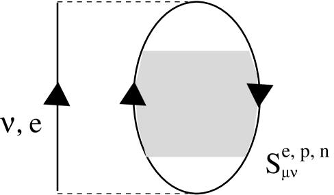
FIG. 2.: The Feynman diagram for the self-energy of neutrino in the Born approximation.The dashed line stands for the weak interaction and the thick lines represent the Green functions for the particles indicated in the figure. The part with a shaded region denotes the structure functions (see the text for definitions) symbolically.

REFERENCES

• [1] J. N. Bahcall, Neutrino Astrophysics, Cambridge University Press, Cambridge, 1989.
• [2] G. Raffelt, Stars as Laboratories for Fundamental Physics, University of Chicago Press, Chicago, 1996.
• [3] S. W. Bruenn, Astrophys. J. Suppl. 58, 771 (1985).
• [4] H. Suzuki, Physics and Astrophysics of Neutrinos, edited by M. Fukugita and A. Suzuki, Springer-Verlag, Tokyo, 1994, p763.
• [5] R. W. Lindquist, Annals of Physics. 37, 487 (1966).
• [6] A. Mezzacappa, and R. A. Matzner, Astrophys. J. 343, 853 (1989).
• [7] S. Yamada, H. -Th. Janka, and H. Suzuki, Astron. & Astrophys. 344, 533 (1999).
• [8] M. Fukugita and T. Yanagida, Physics and Astrophysics of Neutrinos, edited by M. Fukugita and A. Suzuki, Springer-Verlag, Tokyo, 1994, p1.
• [9] M. A. Rudzsky, Astrophysics and Space Sciences 165, 65 (1990).
• [10] G. Raffelt, G. Sigl and L. Stodolsky, Phys. Rev. Lett. 70, 2363 (1993).
• [11] G. Raffelt and G. Sigl, Astropart. Phys. 1, 165 (1993).
• [12] J. Pantaleone, Phys. Lett. B342, 250, (1995).
• [13] J. C. D’Olivo and J. F. Nieves, Int. J. Mod. Phys. A11, 141 (1996).
• [14] M. Sirera and A. PΓ©rez, Phys. Rev. D59, 125011 (1999).
• [15] F. N. Loreti, Y. -Z. Qian, G. M. Fuller and A. B. Balantekin, Phys. Rev. D52, 6664 (1995).
• [16] F. Buccella, S. Esposito, C. Gualdi and G. Miel, Z. Phys. C73, 633 (1997).
• [17] A. Kusenko and G. Segre, Phys. Rev. Lett. 77, 4872 (1996).
• [18] H. -Th. Janka and G. Raffelt, Phys. Rev. D59, 023005 (1999).
• [19] J. Schwinger, J. Math. Phys. 2, 407 (1961).
• [20] L. V. Keldysh, JETP 20 1018 (1965).
• [21] K. -C. Chou, Z. -B. Su, B. -L. Hao and L. Yu, Phys. Rep. 118, 1 (1985).
• [22] P. Danielewicz, Annals of Physics 152, 239 (1984).
• [23] P. D. Mannheim, Phys. Rev. D37, 1935 (1988).
• [24] D. NΓΆtzold and G. Raffelt, Nucl. Phys. B307, 924 (1988).
• [25] S. Esposito and G. Capone, Z. Phys. C70, 55 (1996).
• [26] P. Elmfors, D. Grasso and G. Raffelt, Nucl. Phys. B479, 3 (1996).
• [27] L. P. Kadanoff and G. Baym, Quantum Statistical Mechanics, The Benjamin/Cummings Publishing Company, 1962, London.
• [28] P. J. Schinder, Astrophys. J. Suppl. 74, 249 (1990).
• [29] S. Yamada and H. Toki, Phys. Rev. C61, 015803 (2000).
Refer to caption