Tidal Disruption of a Solar Type Star by a Super-Massive Black Hole

Abstract

We study the long term evolution of a solar type star that is being disrupted by a super massive ($10^{6}$ M_⊙) black hole. The evolution is followed from the disruption event, which turns the star into a long thin stream of gas, to the point where some of this gas returns to pericenter and begins its second orbit around the black hole. Following the evolution for this long allows us to determine the amount of mass that is accreted by the black hole. We find that approximately 75% of the returning mass is not accreted but instead becomes unbound, following the large compression characterizing the return to pericenter. The impact of a tidal disruption on the surrounding gas may therefore be like that of two consecutive supernove-type events.

1 Introduction

It has long been suggested that supermassive black holes (with a black hole mass $M_{\rm bh}\sim 10^{6}$ M_⊙) in relatively low-luminosity active galactic nuclei (AGNs) can be fed by tidal disruptions of stars that are on nearly radial orbits (e.g. Frank, 1978; Lacy et al., 1982; Carter & Luminet, 1985; Rees, 1988, 1990). The frequency of such events is expected to be of the order of $10^{-4}$ yr^-1 in a galaxy like M31. In AGNs with more massive central black holes ($M_{\rm bh}\gtrsim 10^{8}$ M_⊙), stars are “swallowed” whole, since the ratio of the event horizon radius to the tidal disruption radius increases with the black hole mass $\left(\sim M_{\rm bh}^{2/3}\right)$.

Although direct observational evidence for the disruption process is lacking, a few observations have been tentatively identified as being associated with disruption events. For example, an ultraviolet flare at the center of the elliptical galaxy NGC 4552, although rather weak, has been suggested to result from such an event (Renzini et al., 1995). Other sudden eruptions that have been interpreted as potentially resulting from tidal disruptions include outbursts in IC 3599, NGC 5905, RXJ 1242.6-1119, RXJ 1624.9+7554, and RXJ 1331.9-3243 (e.g. Komossa & Greiner, 1999; Komossa & Bade, 1999; Grupe et al., 1999, and references therein). It has also been suggested that the sudden appearance and variability of the double-peaked Balmer lines in the active nucleus NGC 1097 is at least broadly consistent with being produced in a ring resulting from tidal disruption (Storchi-Bergmann et al., 1995). Similarly, it has been proposed that an outburst observed in the Seyfert galaxy NGC 5548 was due to a single star falling into a $\sim 10^{7}$ M_⊙ black hole (Peterson & Ferland 1986; although other interpretations exist, e.g. Terlevich & Melnick 1988; Kallman & Elitzur 1988). More recent work on the broad emission line region of this galaxy, although interesting in its own right, did not shed any new light on the cause of the variability (Goad & Koratkar, 1998).

Several aspects of the problem of stellar encounters with supermassive black holes and of tidal disruption have been examined both analytically and numerically (e.g. Nolthenius & Katz, 1982; Bicknell & Gingold, 1983; Carter & Luminet, 1983; Hills, 1988; Kochanek, 1992, 1994; Syer & Clarke, 1992, 1993; Laguna et al., 1993; Marck et al., 1996). In addition, the interaction of a white dwarf with a massive black hole has been studied both generally (e.g. Frolov et al., 1994) and in the context of gamma-ray bursts (e.g. Fryer et al., 1999).

In the present work, we follow the evolution of a star that is tidally disrupted. In particular, we calculate the properties of the disruption debris to longer times than in some of the previous studies, using a Post-Newtonian, Smooth-Particle-Hydrodynamics (SPH) code.

The numerical method is described in $\S 2$, the results are presented in $\S 3$, and a discussion and conclusions follow.

2 The Numerical Method

We first introduce some notation that will be used throughout the paper. The mass of the black hole is denoted by $M_{\rm bh}$. The gravitational radius of the black hole is $R_{g}=2GM_{\rm bh}/c^{2}$. To measure the strength of the tidal encounter we use the dimensionless parameter (e.g. Press & Teukolsky, 1977)

$$\eta_{t}=\left(\frac{M_{*}}{M_{\rm bh}}\frac{R_{p}^{3}}{R_{*}^{3}}\right)^{1/2}~{}~{},$$ (1)

and to measure the magnitude of the relativistic effects we use

$$\eta_{r}=\frac{R_{p}}{R_{g}}~{}~{},$$ (2)

where $M_{*}$ and $R_{*}$ are the mass and radius of the star respectively and $R_{p}$ is the radius at the pericenter.

Simulating the full evolution of a star that is tidally disrupted by a black hole is a challenging numerical task. Once passing the pericenter, the star is tidally disrupted into a very long and dilute gas stream. As noted already by Kochanek (1994), each fluid element in this stream follows an almost test particle orbit. The fraction of the gas that is bound to the black hole eventually returns to pericenter and moves on to start another orbit. Relativistic orbital precession can cause this outgoing gas stream to collide with the incoming stream. Clearly, this problem consists of highly varying spatial configurations of matter, with much “empty space.” These attributes led to our selection of SPH as the numerical scheme used to tackle this problem. Indeed, previous works that used grid based codes (e.g. Khokhlov et al. (1993b, a); Frolov et al. (1994); Diener et al. (1997)) only followed the star close to the pericenter. This is also true of previous works by Evans & Kochanek (1989), and Laguna et al. (1993) that used SPH.

We use the (0+1+2.5) Post-Newtonian (PN) SPH code described in Ayal et al. (2000). This code implements the formalism of Blanchet, Damour & Schäfer (1990; hereafter BDS) and features full Newtonian gravity and hydrodynamics (0PN), the first order effects of general relativity on the gravity and hydrodynamics [known as the first post-Newtonian, (1PN) approximation], and gravitational wave damping (2.5PN). The independent matter variables used in this formalism consist of the following set: $\rho_{*}$ the coordinate rest mass density, $\varepsilon_{*}$ the coordinate specific internal energy and ${\bf w}$ the specific linear momentum. In fully relativistic terms these are defined as:

$$\rho_{*} = \sqrt{g}u^{0}\rho,$$ (3)

$$\varepsilon_{*} = \varepsilon(\rho_{*}),$$ (4)

$$w_{i} = \left(c^{2}+\varepsilon+p/\rho\right)\frac{u_{i}}{c},$$ (5)

where $\rho$ is the rest mass density, $\varepsilon(\rho)$ is the specific energy, $p(\varepsilon,\rho)$ is the pressure and $u^{\mu}$ is the four-velocity (Greek indices run from 0 to 4, latin indices from 1 to 3). The corresponding BDS variables are the above quantities neglecting all terms except 0PN, 1PN and 2.5PN. Using these variables the formalism yields an evolution system which consists of 9 Poisson equations and 4 hyperbolic equations which we solve as explained in Ayal et al. (2000).

We model the black hole using a massive point particle that has no hydrodynamical interactions. In order to be consistent with the 1PN approximation we must ensure that all the relativistic effects are small (of the order of 10%). This excludes simulating the strong field regions near the black hole’s horizon. We enforce this limit using a fully absorbing boundary condition at $10R_{g}$. Every particle crossing into this region is assumed to be accreted and taken out of the simulation. Since the mass of the star is negligible compared the mass of the black hole, we do not need to increase the mass of the black hole for every particle crossing the $10R_{g}$ boundary.

The statistical nature of SPH does not handle well single, separate particles. Indeed, the entire formalism is built on the assumption that each particle interacts hydrodynamically with about 60 (in 3D) other particles at all times. This number of interactions is needed to form a good sample of the fluid properties for an accurate calculation of gradients. In order to maintain this number of interactions under varying conditions, most SPH codes employ adaptive smoothing lengths (e.g. Benz, 1990; Monaghan, 1992), in effect changing the resolution at each point. In our problem, we have widely varying length scales when the gas stream expands, where varying the smoothing length is advantageous. On the other hand, the difference in the particle eccentricities causes them to separate when approaching pericenter, and they arrive there almost one by one. At this stage, maintaining hydrodynamic interaction with 60 other particles would require huge smoothing lengths, where a small change in the smoothing length would lead to a large change in the number of interactions. This, coupled with an algorithm that tries to maintain a fixed number of interactions, can cause large oscillations in the smoothing length, which in turn introduce a highly varying number of hydrodynamic interactions. These huge smoothing lengths for particles approaching pericenter also mean that we have a very coarse resolution at a crucial stage.

In order to overcome this numerical difficulty we introduce a “particle splitting” (PS) scheme. Whenever a particle satisfies some splitting criterion we split it into new particles each having a smaller mass and smoothing length so that the overall mass is conserved. Thus the PS algorithm consists of two parts—the splitting criterion and the splitting method. In the method we use, maximal splitting, we split each particle into 13 particles, giving the original particle 12 new neighbors (12 is the maximum number of spheres that can “touch” a sphere with the same radius). Another possible method is minimal splitting (while still maintaining a quasi spherical symmetry)—we split each particle into 5, adding 4 particles at the edges of a tetrahedron centered on the original particle. We found that the minimal splitting method tends to produce lumpier particle distributions, we therefore used maximal splitting in both the PS runs presented in this work. We split each particle into 13 particles, each having half the smoothing length of the original particle, spaced by one original smoothing length. This splitting method conserves the particle’s interaction radius which is twice it’s smoothing length. As a splitting criterion we used the ratio between each particle’s smoothing length and the average smoothing length. Whenever the smoothing length of a bound particle exceeds twice the average smoothing length we split this particle. We split only bound particles so as not to waste computational time on the unbound debris, in which we are not interested in the present work. In order for the unbound debris smoothing length not to dominate the average smoothing length which we use for the splitting criterion, we enforce a maximum smoothing length of twice the average smoothing length for unbound particles. This causes unbound particles of gas to have fewer and fewer hydrodynamical interactions, and their motion to be dominated by gravity, as is expected. Another computational time reducing technique that we use is to delete any particle that is both unbound and is farther away than $2500R_{g}$. The latter criterion ensures that the deletion of these particles does not affect the dynamics near pericenter.

In order to estimate the errors in using the particle splitting method, we compared the results of three runs. The first run was a conventional SPH run with a fixed number of 4295 particles, denoted by F1. The second and third runs were PS runs denoted by PS1 and PS2 and they differ only in the number of particles at the initial time. These parameters are summarized in Table 1.

Table 1: The parameters of the three runs. F1 has a fixed number of particles, PS1 and PS2 are particles splitting runs differing only in the number of particles.

Run	Type	Initial # of particles	Maximum # of particles
F1	fixed	4295	4296
PS1	PS	579	1528
PS2	PS	1079	3607

3 Results

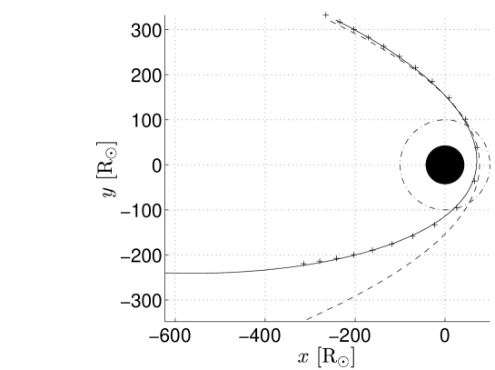
Figure 1: The initial encounter: The star’s CM position near pericenter (crosses), compared with the relativistic orbit (solid line) and Newtonian orbit (dashed line) with the same initial conditions. The black circle in the center has a radius of $10R_{g}$. The dash-dotted line is at the tidal radius. The star’s CM is closer to the relativistic orbit, but it is not precisely on it.

As initial conditions we took a $\Gamma=5/3$ polytrope with a solar radius and mass. This star was then put at a distance of $100R_{g}$ and given the velocity of an appropriate parabolic Keplerian orbit with a pericenter at $20R_{g}$. Giving the initial conditions at such a distance ensures that any relativistic effects (at that position) are negligible so that using Newtonian expressions for various quantities (such as energy) is justified. As can be seen in Fig. 1, the star’s center of mass (CM) follows an almost relativistic orbit, which validates the use of the 1PN approximations for this problem. For this run we obtained the values of $\eta_{r}\approx 18$ and $\eta_{t}\approx 0.65$ at the pericenter. These values ensure that on one hand the 1PN approximation is valid, and on other, that the tidal interaction is sufficiently strong to lead to disruption.

We can roughly divide the disruption process into 2 qualitatively different regimes. In the first, the tidal forces dominate and the star is destroyed. This is followed, at about $t=8$ hours, by the post disruption regime. This latter stage consists of the gas stream phase and the accretions phase. During the gas stream phase the pressure is negligible and the particles move on almost Keplerian orbits. The accretion phase starts at $t=15$ days when the first particles return to pericenter.

3.1 Disruption

The disruption phase for a solar type star was studied, using Newtonian physics, by Evans & Kochanek (1989). Later it was studied in greater detail by Khokhlov et al. (1993b, a); and by Diener et al. (1997) who included a general relativistic treatment of the tidal potential of a Kerr black hole and Newtonian hydrodynamics for the star. This phase was also studied by Laguna et al. (1993) using Newtonian hydrodynamics on a fixed Kerr background. We compare our results for this phase with these previous studies.

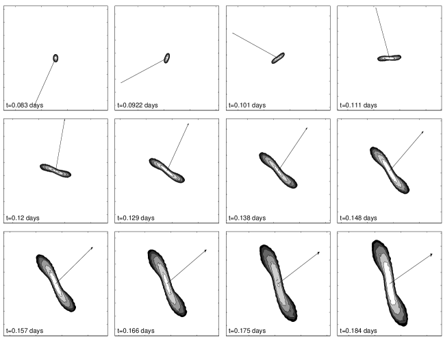
Figure 2: Contours of the rest-mass density on the orbital plane during the disruption. The arrow points to the BH. Time advances from left to right, top to bottom. All figures are to the same scale of 40 R_⊙ per side.

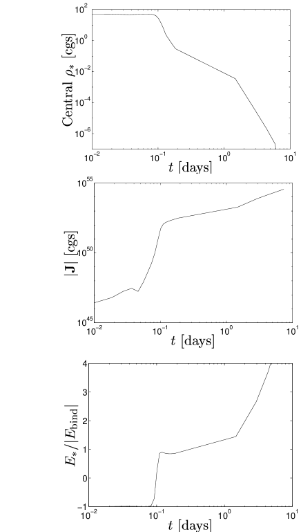
Figure 3: Central coordinate rest mass density $\rho_{*}$, angular momentum $|{\bf J}|$ (relative to the star’s CM), and total energy of the star as a function of time.

The results shown are taken from run F1 which has a higher resolution at this stage. The rest-mass density contours presented in Fig. 2 show the effect of the tidal forces on the star. In Fig. 3 we show the central coordinate rest-mass density $\rho_{*}$, the angular momentum $|{\bf J}|$, and total energy $E_{*}$ of the star, during the disruption. The value of $\rho_{*}$ does not increase beyond the initial value, and it falls rapidly after the disruption. Comparing to Laguna et al. (1993), we find that our encounter is somewhere between a non-relativistic encounter and a single-compression relativistic encounter, as expected. The values of $\rho_{*}$ are also close to those in Diener et al. (1997) and Khokhlov et al. (1993a). The total angular momentum relative to the CM of the star increases by about 5 orders of magnitude at the disruption, and a more gentle increase occurs afterwards, caused by the gravitational torques acting on the debris. The total energy of the star also has a sharp increase at the disruption as the star becomes unbound, followed by another rise as the star moves away from the BH.

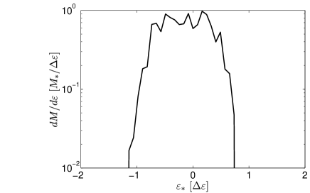
Figure 4: Differential mass distribution in specific energy for the disruption debris

The differential mass distribution in specific energies $dM/d\varepsilon_{*}$ is shown in Fig. 4. We use $\Delta\epsilon=GM_{\rm bh}R_{*}/R_{p}^{2}$, the change in the BH potential across the star (Lacy et al., 1982) as our energy scale. The mass distribution is almost constant as predicted by Rees (1988). A comparison with Evans & Kochanek (1989), who calculated this quantity for the Newtonian case, shows that in our calculation the width of the distribution is smaller by approximately $0.5\Delta\epsilon$ (FWHM).

In general, we find that the 1PN energy $E_{\rm pn}$ is conserved to better than 2%. The energy radiated by gravitational radiation during the disruption is negligible (compared to the total), amounting to $1.6\times 10^{46}$ erg.

3.2 Post Disruption

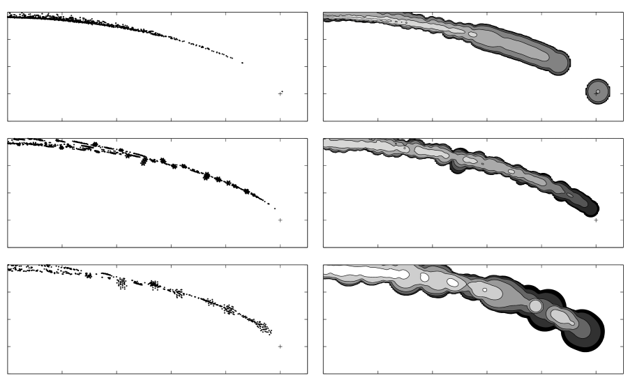
Figure 5: Stream at the beginning of second pericenter passage. On the left, the particle distribution, on the right the density contours. We show the three runs: on the top is the F1 run, in the middle the PS2 run and on the bottom the PS1 run. The width of the plotted area is $10^{4}$ R_⊙. Note that in both the PS runs, the particle density near pericenter is larger than in the F1 run. Also note the isolated particles approaching pericenter in the F1 run, a phenomenon which is absent in the PS runs. The clumping in the particles is produced by the PS scheme.

The post disruption phase begins at about $t=8$ hours. At this stage the gas is sufficiently dilute and cold to make the pressure very small. Consequently, the gas elements in the stream follow almost exact geodesics. A previous study on the gas stream phase, by Kochanek (1994), used the thinness of the stream to decouple the transverse properties of the stream from the variations along its length. This same thinness introduces difficulties into the numerical approach. The spherical nature of the SPH particles causes the code to overestimate the stream width. This effect can be overcome by using more particles but the increase in computational time renders this approach impractical with current hardware. As the SPH particles approach pericenter for the second time, the PS method therefore becomes essential. Without PS, the SPH particles approach pericenter almost one by one and the strong compressional effects are manifested through two- and three-particle interactions near the pericenter. This small number of interactions could reduce the reliability of the results. By using PS however, we increase the number of particles approaching pericenter, thus increasing the number of interactions and thereby ensuring that the hydrodynamical interactions remain adequate. The effects of PS can be seen in Fig. 5 where the conventional run has a very non-uniform particle density even when compared to the PS1 run (with only 1350 particles at this stage).

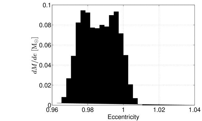
Figure 6: The eccentricity distribution of the gas in the stream just before the first particle approaches pericenter (at $t\approx 15\rm days$). The mean eccentricity is $\approx 0.994$.

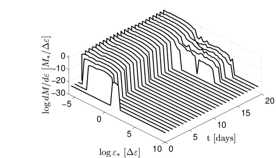
Figure 7: Differential mass distribution in specific internal energy for the disruption debris as a function of time.

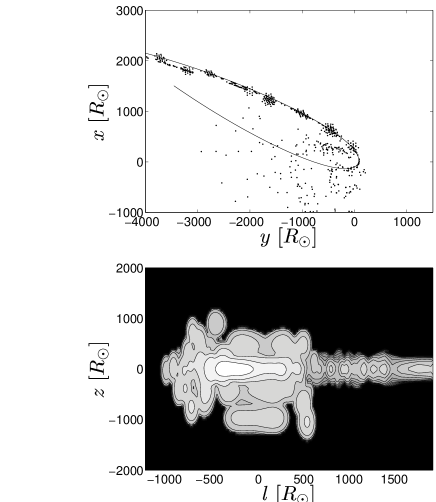
Figure 8: Pressure along a path. At the top we show the path, chosen to pass through the gas stream and pericenter. At the bottom we show logarithmic contours of the pressure. The contours are spaced by one decade. $l$ is the length parameter of the path, $l=0$ corresponds to the point where the path intersects the $x$ axis, near pericenter and $l$ grows counter-clockwise.

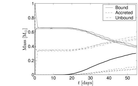
Figure 9: Bound, accreted and unbound mass as a function of time. For each type of mass there are two lines for the two runs. As can be seen, the maximal difference is $\approx 10$%. The heavy solid line is the accreted mass as predicted by assuming that all the returning mass is accreted.

In Fig. 6 we show the distribution of eccentricities for the SPH particles in the gas stream phase. The mean eccentricity is about 0.994, as the star was initially marginally bound. The distribution does not change by much until the end of the stream phase, when the first particle approaches pericenter. The differential mass distribution in specific internal energy as a function of time is shown in Fig. 7. The earliest time shown is close to that of Fig. 4. As can be seen, at the gas stream phase the internal energy distribution shifts towards lower energies, while the second passage through pericenter heats the particles up. This heating is caused by the strong compression characterizing the second passage of the gas through pericenter. The compression is caused by the gas orbits converging to the space occupied by the star at the initial pericenter (e.g. Kochanek, 1994). This compression can be seen in Fig. 8 where we show the pressure at some fixed time after the first return to pericenter in the PS2 run. The pressure is shown along a path as a function of $l$, the length of the path. The path was chosen so as to pass through the gas stream and pericenter. As can be seen, the pressure rises sharply at negative $l$, corresponding to the passage through pericenter, and there is a large pressure gradient in the $z$ direction. We find that the bounce that follows this compression is sufficiently strong to impart a significant fraction of the gas with the escape velocity. In Fig. 9 we show the amount of the star’s mass that is bound, unbound, and accreted (we note again that accreted here means that it has come closer then $10R_{g}$ to the BH). As the star leaves the vicinity of the BH for the first time, 65% of its mass is bound. This stays constant during the gas stream phase since the pressures are small. Following the second passage through pericenter however, mass gets unbound, until, at the time we stop our simulation, 50% of the mass is unbound, 40% is bound and the remaining 10% is accreted. The relative difference between the two runs is about 10% in all of these quantities.

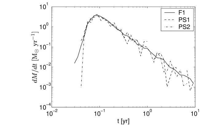
Figure 10: Differential mass distribution in orbital period for the bound mass. The PS runs have less particles at this stage than the F1 run (870, 2040 and 4295 particles for the PS1, PS2 and F1 runs respectively) at this stage so the distribution is less smooth, especially in the long period masses. Both runs display a similar distribution near the maximum and up to $0.2{\rm~{}yr}$, when we stop the simulation.

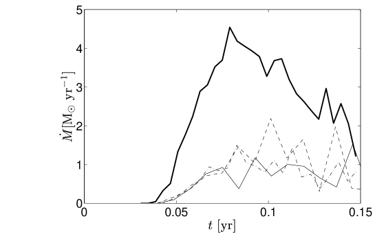
Figure 11: Accretion rates. The solid line is the accretion rate assuming that all the returning mass is accreted; the other three lines are the actual accretion rate for the three runs.

In Fig. 10 we show the differential mass distribution in orbital periods in the stream. This has been used in previous works (e.g. Rees, 1988; Evans & Kochanek, 1989; Laguna et al., 1993) to estimate the mass infall rate onto the BH, under the assumption that all the mass returning to pericenter is accreted. In Fig. 11 we show the estimated accretion rate according to Fig. 10 together with the actual accretion rate we get. Our calculations show that since some of the mass becomes unbound when reaching pericenter, the actual accretion rate is a factor of 3 lower than that inferred previously. The total accreted mass up to 60 days (Fig. 9) was overestimated by a factor of 4 when assuming that all returning mass is accreted. Another important consequence of the strong compression near pericenter is that the expected self-intersection of the gas stream in fact does not occur, since the debris is given a high velocity perpendicular to the orbital plane.

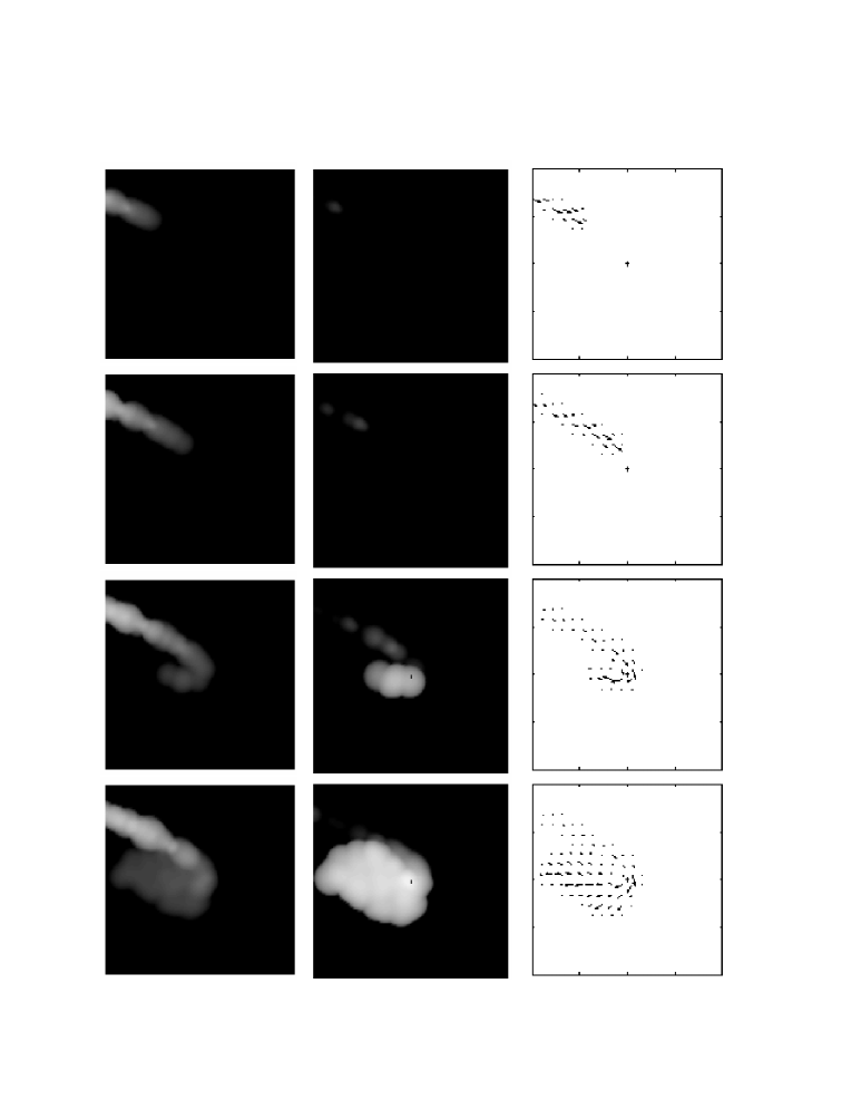
Figure 12: On the left logarithm of the density, in the middle, logarithm of the specific internal energy and on the right velocity components for various times during the return to pericenter. Results are taken from the PS2 run. The BH is at the center, the box size is 2000 R_⊙.

The inner $10^{4}$ R_⊙ around the BH is composed of the infalling debris and a low density cloud with a density of $\approx 10^{-11}~{}{\rm g~{}cm^{-3}}$ and with a temperature range of higher than $10^{6}$ K. In Figs. 12 and 13 we show the density, specific internal energy and velocity in the inner 2000 R_⊙ around the BH. Even using PS is is clear that we cannot resolve structures well within this radius (e.g. an accretion disk, as proposed by Cannizzo et al. 1990). Nevertheless, there is some evidence of circularization of the gas flow in the velocity plots.

4 Discussion

We have performed a 1PN simulation of a solar mass star being disrupted by a super massive ($10^{6}$ M_⊙) black hole. The disruption process itself causes about 1/2 of the star’s matter to become unbound. We follow this matter up to and beyond the time when it returns to pericenter and starts accreting onto the BH. This in turn enables us to determine the amount of returning mass that is actually accreted. Contrary to previous, more heuristic estimates, we find that only about 25% of the returning mass actually gets accreted. The rest becomes unbound, following being heated by the strong compression accompanying the approach to pericenter.

The main consequence of this process is that the maximum accretion rate is a factor of 3 lower than expected from a simple examination of the rate of mass return to pericenter. The accretion rate into the volume resolved by our simulation is also quite constant, at about 1 ${\rm M_{\odot}~{}yr^{-1}}$, for the last 20 days of the simulation as opposed to a power law decay which is expected from the rate of return. When integrated over time, these results show that only about 10% of the original star’s mass actually gets accreted as opposed to the 65% expected if all the bound mass would be finally accreted. This means that the mass involved in the accretion flow, be it in the form of an accretion disk (e.g. Cannizzo et al., 1990), or spherical accretion (e.g. Loeb & Ulmer, 1997) is considerably smaller than previously estimated. Consequently, the duration of the expected ‘flare’ can be shorter by a factor 4–5 compared to these early estimates, which makes the detectability of these events much harder (the rather high temperature of some of the infalling debris also makes the bolometric correction high). Indeed, supernova searches in distant galaxies have failed so far to identify any such event unambiguously (Filippenko 2000, private communication).

The mass of the debris that becomes unbound because of the pericenter compression is comparable to the mass of the unbound debris resulting from the original disruption event. The main difference is that this new debris component has a different orbital distribution. Most notably, the velocity has a much larger component in the direction perpendicular to the orbital plane. This additional component of unbound high velocity debris could produce interesting consequences (e.g. components like Sgr A East in the Galactic center) when colliding with the interstellar medium surrounding the BH (e.g. Khokhlov & Melia, 1996). In particular, the fact that the mass ejection is more spherically symmetric, makes the event more similar to a normal supernova. Thus, tidal disruption events may produce a quite unique signature (in terms of their impact on surrounding gas), in which two supernova-type events are separated by a few weeks to a few months, with the first one being very anisotropic (mass being ejected within a solid angle $\Omega\ {\raise-2.15277pt\hbox{$\buildrel>\over{\sim}$}}\ 16(R_{*}/R_{\rho})^{1/2}(M_{*}/M_{\rm bh})^{1/2}$ rad²) and the second more spherically symmetric.

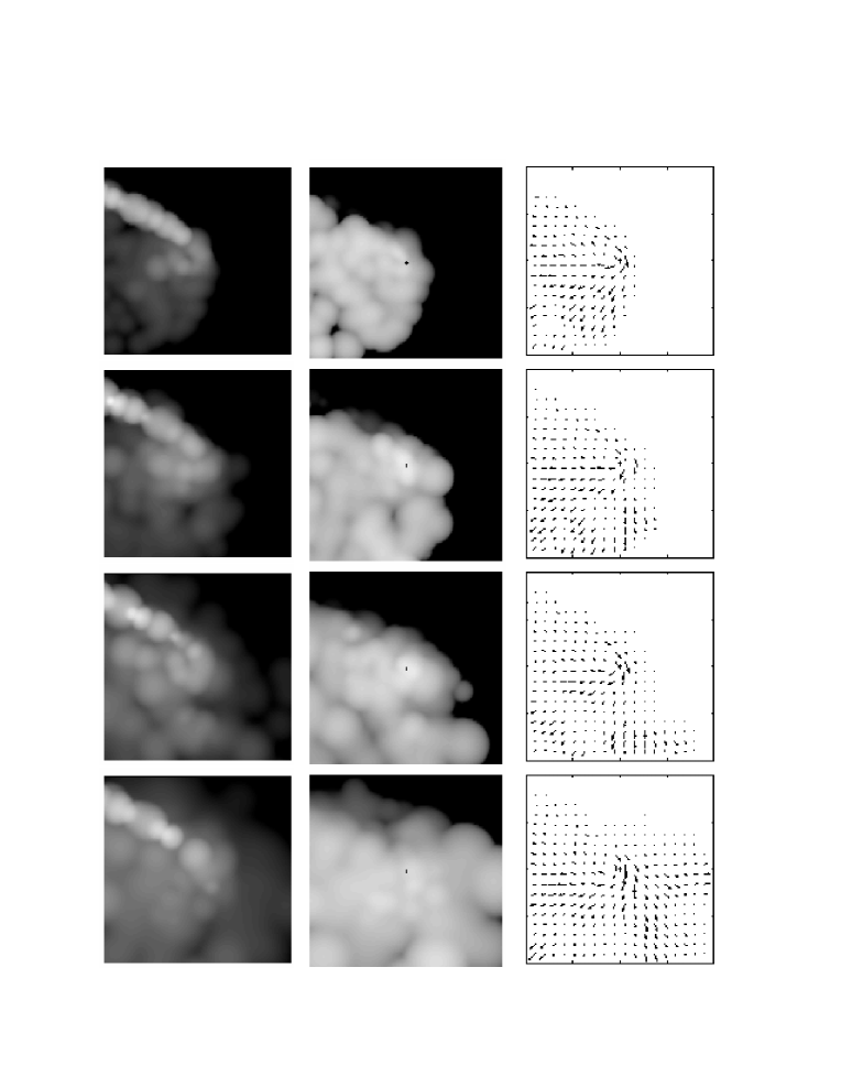
Figure 13: More frames like Fig. 12.

References

- Ayal et al. (2000) Ayal, S., Piran, T., Oechslin, R., Davies, M. B., & Rosswog, S. 2000, ApJ, submitted
- Benz (1990) Benz, W. 1990, in The Numerical Modeling of Nonlinear Stellar Pulsations: Problems and Prospects, ed. J. R. Buchelr (Dordrecht: Kluwer), 269–288
- Bicknell & Gingold (1983) Bicknell, G. V. & Gingold, R. A. 1983, ApJ, 273, 749
- Blanchet et al. (1990) Blanchet, L., Damour, T., & Schaefer, G. 1990, MNRAS, 242, 289
- Cannizzo et al. (1990) Cannizzo, J. K., Lee, H. M., & Goodman, J. 1990, ApJ, 351, 38
- Carter & Luminet (1983) Carter, B. & Luminet, J.-P. 1983, A&A, 121, 97
- Carter & Luminet (1985) Carter, B. & Luminet, J. P. 1985, MNRAS, 212, 23
- Diener et al. (1997) Diener, P., Frolov, V. P., Khokhlov, A. M., Novikov, I. D., & Pethick, C. J. 1997, ApJ, 479, 164+
- Evans & Kochanek (1989) Evans, C. R. & Kochanek, C. S. 1989, ApJ, 346, L13
- Frank (1978) Frank, J. 1978, MNRAS, 184, 87
- Frolov et al. (1994) Frolov, V. P., Khokhlov, A. M., Novikov, I. D., & Pethick, C. J. 1994, ApJ, 432, 680
- Fryer et al. (1999) Fryer, C. L., Woosley, S. E., Herant, M., & Davies, M. B. 1999, ApJ, 520, 650
- Goad & Koratkar (1998) Goad, M. & Koratkar, A. 1998, ApJ, 495, 718+
- Grupe et al. (1999) Grupe, D., Thomas, H. ., & Leighly, K. M. 1999, A&A, 350, L31
- Hills (1988) Hills, J. G. 1988, Nature, 331, 687
- Kallman & Elitzur (1988) Kallman, T. & Elitzur, M. 1988, ApJ, 328, 523
- Khokhlov & Melia (1996) Khokhlov, A. & Melia, F. 1996, ApJ, 457, L61
- Khokhlov et al. (1993a) Khokhlov, A., Novikov, I. D., & Pethick, C. J. 1993a, ApJ, 418, 181+
- Khokhlov et al. (1993b) —. 1993b, ApJ, 418, 163+
- Kochanek (1992) Kochanek, C. S. 1992, ApJ, 385, 604
- Kochanek (1994) —. 1994, ApJ, 422, 508
- Komossa & Bade (1999) Komossa, S. & Bade, N. 1999, A&A, 343, 775
- Komossa & Greiner (1999) Komossa, S. & Greiner, J. 1999, A&A, 349, L45
- Lacy et al. (1982) Lacy, J. H., Townes, C. H., & Hollenbach, D. J. 1982, ApJ, 262, 120
- Laguna et al. (1993) Laguna, P., Miller, W. A., Zurek, W. H., & Davies, M. B. 1993, ApJ, 410, L83
- Loeb & Ulmer (1997) Loeb, A. & Ulmer, A. 1997, ApJ, 489, 573+
- Marck et al. (1996) Marck, J. A., Lioure, A., & Bonazzola, S. 1996, A&A, 306, 666+
- Monaghan (1992) Monaghan, J. J. 1992, ARA&A, 30, 543
- Nolthenius & Katz (1982) Nolthenius, R. A. & Katz, J. I. 1982, ApJ, 263, 377
- Peterson & Ferland (1986) Peterson, B. M. & Ferland, G. J. 1986, Nature, 324, 345
- Press & Teukolsky (1977) Press, W. H. & Teukolsky, S. A. 1977, ApJ, 213, 183
- Rees (1988) Rees, M. J. 1988, Nature, 333, 523
- Rees (1990) —. 1990, Science, 247, 817
- Renzini et al. (1995) Renzini, A., Greggio, L., di Serego-Alighieri, S., Cappellari, M., Burstein, D., & Bertola, F. 1995, Nature, 378, 39+
- Storchi-Bergmann et al. (1995) Storchi-Bergmann, T., Eracleous, M., Livio, M., Wilson, A. S., Filippenko, A. V., & Halpern, J. P. 1995, ApJ, 443, 617
- Syer & Clarke (1992) Syer, D. & Clarke, C. J. 1992, MNRAS, 255, 92
- Syer & Clarke (1993) —. 1993, MNRAS, 260, 463+
- Terlevich & Melnick (1988) Terlevich, R. & Melnick, J. 1988, Nature, 333, 239+