Abstract

The evolution of the star formation rate in the Galaxy is one of the key ingredients quantifying the formation and determining the chemical and luminosity evolution of galaxies. Many complementary methods exist to infer the star formation history of the components of the Galaxy, from indirect methods for analysis of low-precision data, to new exact analytic methods for analysis of sufficiently high quality data. We summarise available general constraints on star formation histories, showing that derived star formation rates are in general comparable to those seen today. We then show how colour-magnitude diagrams of volume- and absolute magnitude-limited samples of the solar neighbourhood observed by Hipparcos may be analysed, using variational calculus techniques, to reconstruct the local star formation history. The remarkable accuracy of the data coupled to our maximum-likelihood variational method allows objective quantification of the local star formation history with a time resolution of $\approx 50$Myr. Over the past 3Gyr, the solar neighbourhood star formation rate has varied by a factor of $\sim$4, with characteristic timescale about 0.5Gyr, possibly triggered by interactions with spiral arms.

1 Star Formation Rates: Qualitative Deductions

Star formation rates and histories can be estimated in special cases from a combination of chemical evolution models and the total stellar mass formed into stars. Basically, this exploits the stellar evolutionary, and Type I supernova timescales for element production. One requires that stars formed at a rate consistent with their chemical distributions, whether a $\delta$-function, a range in the products of both Type I and Type II supernaova, products of single supernovae with time for efficient mixing of the ISM, or whatever. Combining these albeit crude estimates of the duration of star formation with a calculation of the stellar mass formed, provides a star formation rate. Perhaps surprisingly, given the crude calculation, such derived rates are both similar to those determined more accurately today, and are all quite low.

TABLE 1.  : A summary of star formation rates, and durations of star formation, in some Galactic stellar populations. These values are derived from combination of chemical element scatter and masses.

  Population Duration Formation Rate   (years) ${\mathcal{M}}_{\odot}yr^{-1}$   Globular cluster $\leq 10^{8}$ $\geq 0.01$ $\omega$Cen $\geq 10^{8}$ $\leq 0.1$ Halo, [Fe/H]$\leq-2.0$ $\leq 10^{8}$ $\sim 1$ Halo, [Fe/H]$\sim-1.5$ $\leq 10^{9}$ $\sim 1$ Bulge; high [$\alpha$/Fe] few.10⁸ 10-100 Bulge; low [$\alpha$/Fe] few.10⁹ 10-100 Thick Disk few.10⁹ 1-10 Current Disk $10^{10}$ $\sim 1-10$ Inner Disk ? ? Satellite dSph many.10⁹ $\leq 10^{-3}$    Assembly   early  
 
Infall continuing? $\sim 4$Gyr
 

In cases where no spread in element ratios is seen, and there is no range in [Fe/H], star formation was plausibly complete before new chemical elements could be produced; perhaps globular clsuters are an example of this case. For field halo stars with [Fe/H]$\geq-2$, where a wide range in [Fe/H] but a very small range in [$\alpha$/H] is seen, star formation must have continued for long enough for efficient mixing of supernova ejecta into the ISM. Since no products of Type I supernovae are seen, this brackets allowed star formation durations. By applying such qualitative considerations, we deduce that most of the Milky way formed at a star formation rate which is comparable to that of today. Only the Galactic Bulge, and the inner disk, where star formation histories remain very poorly known, are available to retrieve the Milky Way’s place as a ‘typical object’ on the Madau plot. These simple calculations are summarised in Table (1).

2 Quantitative Determination of Star Formation Rates

Most attempts at deducing the past history of the star formation rate in the Galaxy have relied on indirect age indicators, typically chemical evolution models, using an age-metallicity relation, or from empirical correlations of stellar properties, such as chromospheric activity, with age. Because of the many uncertainties and observational biases inherent in these methods, many corrections must be applied to the samples before a SFH can be inferred. A good recent example, illustrating the strengths and complexities of the techniques, is Rocha-Pinto et al. (2000). Given all this, it is not too surprising to find conflicting results from independent analyses of the limited available data.

The precision in luminosities of field stars provided by the Hipparcos satellite gives us for the first time the data quality to allow application of a more objective method to infer the star formation history which produced the solar neighbourhood. Indeed, recent analytical developments show that it is now possible to reconstruct the star formation history which gave rise to the observed distribution of stars in the HR diagram for any (relatively) simple stellar population. The constraints in present application of the methodology are that one requires (i) a small scatter in the metallicity distribution, and known mean abundance, (ii) a colour-magnitude diagram extending below the turnoff age of interest, and (iii) appropriate stellar evolutionary tracks. Whilst previous reconstructions of the star formation history based on the inversion of CMDs were forced to rely on assumed parametric forms for the evolution of the star formation rate, we have developed and implemented a new and rigorous method which makes no a priori assumptions about the possible complexity of the star formation history.

This method is explained in detail in Hernandez et al. (1999, Paper I) and in Gilmore etal. (2000). These references also present results from the extensive simulations which were used to quantify the biases inherent in any reconstruction based on observational colour-magnitude data. The effects of unresolved binaries, of uncertainties in the stellar initial mass function, and of errors in the adopted system metallicity, were assessed. It was concluded that derivation of an absolute normalisation of the derived star formation rate is still not robust, given the uncertainties in the distribution of mass ratios in binaries, of the fraction of binaries in a given sample, of the IMF, and of metallicity distributions. However, a relative star formation history can be inferred, where the relative amplitudes of the variations in star formation rate are correct, provided the IMF, the properties of binaries and the distribution of metallicity do not evolve with time. With these provisos, the method was applied to a sample of HST CMDs of dSph galaxies of the Local Group (Hernandez, Gilmore, & Valls-Gabaud 2000, Paper II). A further paper extends the application to the Solar neighbourhood (Hernandez, Valls-Gabaud & Gilmore 2000, Paper III).

Full details of the method are presented in Paper I, and in Gilmore et al. (2000), and will not be repeated here. Very briefly, the method takes as inputs only the positions of $n$ stars in a colour magnitude array, each having a colour $c_{i}$ and luminosity $l_{i}$, with (uncorrelated) associated errors $\sigma(c_{i})$ and $\sigma(l_{i})$ respectively. Using the likelihood technique, we first construct the probability that the $n$ observed stars resulted from some function $SFR(t)$. This is given by

$${\cal L}=\prod_{i=1}^{n}\left(\int_{t_{0}}^{t_{1}}\,SFR(t)\,G_{i}(t)\,dt\right),$$ (1)

where

$$G_{i}(t)=\int_{m_{0}}^{m_{1}}{\rho(m;t)\over{2\pi\sigma(l_{i})\sigma(c_{i})}}\,\exp\left(-D(l_{i};t,m)^{2}\over{2\sigma^{2}(l_{i})}\right)\exp\left(-D(c_{i};t,m)^{2}\over{2\sigma^{2}(c_{i})}\right)\hskip 5.0ptdm$$ (2)

In the above expression $\rho(m;t)$ is the density of points along the isochrone of age $t$, around the star of mass $m$. It is determined by convolving an assumed IMF with a stellar evolutionary track, defining the duration of the differential evolutionary phases for a star of mass $m$. The ages $t_{0}$ and $t_{1}$ are a minimum and a maximum age which need to be considered in the specific problem of interest, while $m_{0}$ and $m_{1}$ are a minimum and a maximum mass which need to be considered along each isochrone, typically 0.6${\mathcal{M}}_{\odot}$ and 20${\mathcal{M}}_{\odot}$. $D(l_{i};t,m)$ and $D(c_{i};t,m)$ are the differences in luminosity and colour, respectively, between the $i$th observed star and a general star of age and mass $(m,t)$. We refer to $G_{i}(t)$ as the likelihood matrix, since each element represents the probability that a given star, $i$, was actually formed at time $t$ with any mass.

Following the discussion of Paper I, we may write the condition that the likelihood has an extremal as the variation $\delta{\cal L}(SFR)=0$, allowing a full variational calculus analysis to be applied. Developing first the product over $i$ using the chain rule, and dividing the resulting sum by ${\cal L}$, one obtains:

$$\sum_{i=1}^{n}\left({\delta\int_{t_{0}}^{t_{1}}SFR(t)\,G_{i}(t)\,dt}\over{\int_{t_{0}}^{t_{1}}SFR(t)\,G_{i}(t)\,dt}\right)=0$$ (3)

Introducing the new variable $Y(t)$ defined as:

$$Y(t)=\int{\sqrt{SFR(t)}\,dt}\;\Longrightarrow\;SFR(t)=\left({dY(t)\over dt}\right)^{2}$$

into Equation (2) we can develop the Euler equation to yield

$${d^{2}Y(t)\over dt^{2}}\sum_{i=1}^{n}\left(G_{i}(t)\over I(i)\right)=-{dY(t)\over dt}\sum_{i=1}^{n}\left(dG_{i}/dt\over I(i)\right)$$ (4)

where

$$I(i)=\int_{t_{0}}^{t_{1}}SFR(t)\,G_{i}(t)\,dt$$

We have now transformed what was an optimisation problem, finding the function that maximises the product of integrals defined by equation (1), into an integro-differential equation with a boundary condition (at either $t_{o}$ or $t_{1}$) which can be solved by iteration. Further details on the numerical aspects of the procedure are available in Paper I, and need not be repeated here.

This methodology has two important advantages over traditional maximum likelihood techniques:
(i) variational calculus allows a fully non-parametric approach, independent of one’s astrophysical pre-conceptions; and
(ii) since the optimal star formation history $SFR(t)$ is solved for directly, the computational procedure is very fast, not requiring repeated CPU intensive comparisons between observed and synthetic diagrams.

3 Objective Determination of Recent Star Formation Histories

We now apply the methodolgy outlined above to the Solar Neighbourhood. A suitable data set can be derived from the Hipparcos catalogue (ESA 1997), providing absolute luminosities and colours which are, with careful selection, are almost bias-free. The sample is however restricted to bright stars, and so samples only a very small volume, and releatively young ages. We have derived from the Hipparcos catalogue a volume-limited survey of the solar neighbourhood. This selection is described in detail in Paper III, along with the kinematic and geometrical corrections that have to be made to correct the sample for its selection function.

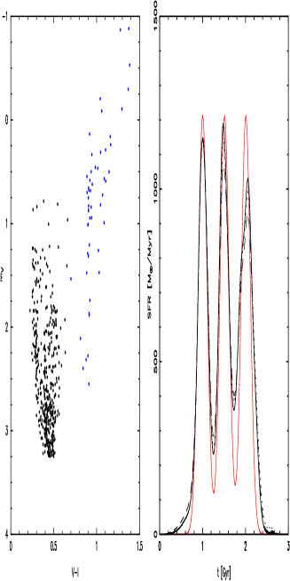
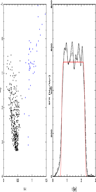
Figure 1.  : Proving the method with a series of 3 bursts of star formation. The synthetic CMD (left panel) results from the 3-burst star formation history shown by the dotted line in the right panel. The solid lines on the right panel are the last three iterations of the inversion, given no information except the CMD of the left panel, and an appropriate metallicity. An accurate reconstruction of the star formation history is apparent. This simulation utilises the same number of stars and the same observational uncertainties as in the Hipparcos sample.

Figure 2.  : Same as Figure 1, except that the simulated CMD is derived from a constant SFR over several Gyr (dotted curve, right hand panel). Note that the CMD appears superficially very similar to the one presented in Fig. 1, even though the simulated star formation history is quite different. The method implemented here is able to distinguish and recover the correct (test) star formation histories.

In summary, we restrict consideration to non-variable stars with apparent magnitude brighter than $V=7.9$ and error in parallax smaller than 20%. To avoid a wide distribution in the uncertainties in colour and luminosity the sample is further reduced to absolute magnitudes brighter than $M_{V}=3.15$. This absolute magnitude-limited sample implies that only stars younger than about 3 Gyr are considered. Determination of the star formation history of the Galactic disk at earlier times awaits a deeper sample, such as will be naturally provided by the GAIA mission.

3.1 Simulations and calibrations

This analysis extends the temporal resolution of the method to much shorter times than used in the simulations described in Paper I. In order to check whether samples such as the one selected can in fact be inverted to infer their star formation history with extremely high temporal resolution, we performed a further extensive set of of tests. As before, these involved creation, convolution with an error and sampling function, and objective inversion, of colour magnitude data resulting from a variety of complex star formation histories. Figure 1 illustrates one such test, where a series of 3 bursts (right panel, dashed line) gives rise to the synthetic CMD shown on the left. The solid lines in the right panel give the last 3 iterations of the method, showing convergence to an accurate reconstruction of the input star formation history.

Similarly, Figure 2 shows a test with a constant star formation rate continuing over several Gyrs. The small fluctuations in the reconstructed star formation history arise from numerical instabilities created by the shot noise due to the small number of stars involved, about 450. This implies that a smoothing procedure has to be applied, resulting in a degradation in the effective time resolution to about 50 Myr. Note also that only stars bluewards of $V-I$=0.7 are used, to avoid unnecessary complications created by a small number of potentially older stars with an extremely poorly quantified selection function contaminating the reconstruction.

4 Star Formation History of the Solar Neighbourhood

Figure (3) shows the colour magnitude diagram for those stars in the volume-limited sample complete to $M_{V}<3.15$ for stars in the Hipparcos catalogue having errors in parallax of less than $20\%$ and with apparent magnitude $m_{V}<7.25$ (left panel). The right panel of this figure shows the result of applying our inversion method to this data set. The dotted envelope spanning the best-fit star formation history quantifies the range of many reconstructions arising from different $M_{V}$ selection cuts in the Hipparcos catalogue. This quantifies the plausible range of systematic errors likely to be present, due predominately to the small sample of stars, and the inevitably a posteriori selection function which must be applied to Hipparcos data. Reconstruction based on the $(M_{V},B-V)$ diagram rather than $(M_{V},V-I)$ gives essentially the same results, showing that the available isochrones are a good match to the photometric systems.

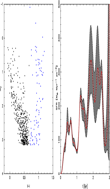
Figure 3.  : The left panel shows the colour magnitude data for the complete sample of nearby massive stars with good parallaxes from Hipparcos. The right panel presents a best-fit reconstruction of the star formation history (solid line), along with the envelope resulting from reconstructions with different $M_{V}$ cuts, to assess the robustness of the inferred star formation history. The decrease to zero at recent times is an artefact of the very small sampling volume.

The derived local star formation history of the Solar Neighbourhood shown in Figure (3) shows what may be described as an underlying constant level of star formation activity, onto which is superimposed a strong, quasi-periodic variation with a period close to $0.5$ Gyr. The high time resolution of our star formation history reconstruction makes it difficult to compare with the results derived from chromospheric activity studies (eg Rocha-Pinto et al. 1999), although qualitatively we do find the same activity at both 0.5 and above 2 Gyr, but not the decrease found by them between 1 and 2 Gyr.

Assuming the variable component really is a cyclic pattern superimposed on a base level, and that our brief time interval is sufficient to identify a true characteristic ‘period’, we may consider its meaning. One possible interpretation of a cyclic component, or at least of some temporal regularity in the star formation history of the solar neighbourhood, can be found in the density wave hypothesis (Lin and Shu, 1964) for the presence of spiral arms in late type galaxies. As the pattern speed and the circular velocity are in general different, the solar neighbourhood periodically crosses an arm region, where the increased local gravitational potential might possibly trigger an episode of star formation. In this case, the time interval $\Delta t$ between encounters with an arm at the solar neighbourhood is

$$\Delta t\;=\;\frac{0.22\,{\rm Gyr}}{m}\;\left(\frac{\Omega}{29\,{\rm km\,s}^{-1}{\rm kpc}^{-1}}\right)^{-1}\;\left|\frac{\Omega_{p}}{\Omega}-1\right|^{-1}$$

where $m$ is the number of arms in the spiral pattern. The classical value of the pattern speed, $\Omega_{p}=0.5\,\Omega\approx 14.5$km s^-1 kpc^-1 would imply the rather surprising conclusion that interaction with a single arm ($m=1$) would be enough to account for the observed regularity in the recent SFR history.

However, more recent determinations tend to point to much larger values for the pattern speed (e.g. Mishkurov et al. 1979, Avedisova 1989, Amaral and Lépine 1997) close to $\Omega_{p}\sim 23-24$ km s^-1 kpc^-1, which would then imply that the regularity present in the reconstructed $SFR(t)$ would be consistent with a scenario where the interaction of the solar neighbourhood with a two-armed spiral pattern would have induced the star formation episodes we detect. This is reminiscent of the explanations put forward to account for the inhomogeneities observed in the HIPPARCOS velocity distribution function, where well-defined branches associated with moving groups of different ages (Chereul et al. 1999, Skuljan et al. 1999, Asiain et al. 1999) could perhaps be also associated with an interaction with spiral arm(s), although in this case the time scales are much smaller. Of course, other explanations are possible; for example the cloud formation, collision and stellar feedback models of Vazquez & Scalo (1989) predict a phase of oscillatory star formation rate behaviour as a result of a self-regulated star formation régime. Close encounters with the Magellanic Clouds have also been suggested to explain the intermittent nature of the star formation rate, though on longer time scales (Rocha-Pinto et al. 2000).

4.1 Are the Results Reliable?

The first question that arises upon application of any new technique, especially one involving complex numerical optimisations, is how reliable is the reconstruction of the star formation history we have deduced? The most common procedure to compare a specific star formation history with an observed CMD has been to use the star formation history to generate a synthetic CMD, and then to compare this to the observations, using some statistical test to determine the degree of similarity between the two.

This method has a significant disadvantage in the present case, in that one is not comparing the ‘true’ star formation history with the data, but rather a particular realisation of the star formation history is being compared with the data. The distinction becomes arbitrary only when large numbers of stars are found in all regions of the colour magnitude diagram. This is not true in general, and especially not so in this application. Instead we follow a Bayesian approach, and adopt for use here the $W$ statistic presented by Saha (1998). This is essentially

$$W=\prod_{i=1}^{B}{{(m_{i}+s_{i})!}\over{m_{i}!s_{i}!}}$$

where B is the number of cells into which the CMD is split, and $m_{i}$ and $s_{i}$ are occupation numbers, the numbers of points which the two distributions being compared have in each cell. This asks for the probability that two distinct data sets are random realisations of the same underling distribution.

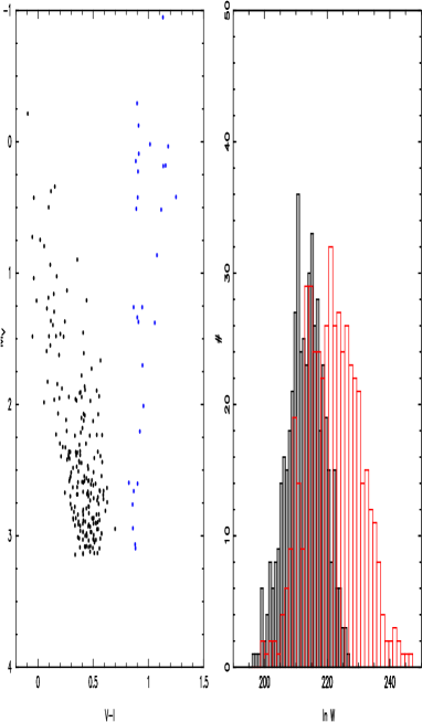
Figure 4.  : The left panel shows one synthetic colour magnitude distribution resulting from the reconstructed star formation history of Fig. 3 (left panel), generated with the same selection function as for the observed Hipparcos sample. The right panel shows the distribution of the $W$ statistic for 500 model-model comparisons (solid lines), illustrating the range of the $W$ statistic expected from sampling statistics, given a fixed underlying star formation function. The dashed line shows the $W$ statistics resulting from 500 comparisons of simulated models and the actual Hipparcos data, from Figure (3). The overlap between the two sets of results shows that the derived star formation history of Figure (3) is indeed a statistically valid representation of the data.

In implementing this test we first produce a large number of random realisations of the colour magnitude diagram generated by our inferred star formation history, and then compute the $W$ statistic between pairs in this sample of CMDs. This gives a distribution which is used to determine the range of values of $W$ which is expected to arise in random realisations of the star formation history being tested. Next, we produce a new set of a large number of random realisations of the colour magnitude diagram generated by our inferred star formation history, and compute the $W$ statistics between the observed data set and these new random realisations of the star formation history. This gives a new distribution of $W$, which can then be objectively compared to the one arising from the model-model comparison. This allows us to assess whether both data and modeled colour magnitude diagrams are compatible with a unique underling distribution.

Figure (4) shows one such synthetic colour magnitude diagram produced from our inferred star formation history for the solar neighbourhood, down to $M_{V}=3.15$. This can be compared to the Hipparcos CMD complete to the same $M_{V}$ limit shown in Figure (3). A visual inspection reveals approximately equal numbers of stars in each of the distinct regions of the diagram. Such a comparison is of little value, however, as noted in dicussion of the simulations summarised in Figures (1) & (2). A rigorous statistical comparison is also possible. The right panel of Figure (4) shows a histogram of the values of the $W$ statistic for 500 random realisations of our inferred star formation history in a model-model comparison. This gives the probability density function for the $W$, given our star formation history. The dashed histogram presents the result of the comparison of 500 synthetic colour magnitude diagrams with the observed Hipparcos data set: both sets of $W$ are compatible.

5 Conclusion

Star formation rates and histories can be estimated in special cases from a combination of chemical evolution models and the total stellar mass formed into stars. Basically, this exploits the stellar evolutionary, and Type I supernova timescales for element production. In cases where no spread in element ratios is seen, and there is no range in [Fe/H], star formation was plausibly complete before new chemical elements could be produced; perhaps globular clsuters are an example of this case. For field halo stars with [Fe/H]$\geq-2$, where a wide range in [Fe/H] but a very small range in [$\alpha$/H] is seen, star formation must have continued for long enough for efficient mixing of supernova ejects into the ISM. Since no products of Type I supernovae are seen, this brackets allowed star formation durations. By applying such qualitative considerations, we deduce that most of the Milky way formed at a star formation rate which is comparable to that of today. Only the Galactic Bulge, and the inner disk, where star formation histories remain very poorly known, are available to retrieve the Milky Way’s place as a ‘typical object’ on the Madau plot.

In the immediate Solar neighbourhood, and in dSph satellite galaxies, the high quality data and the simple stellar populations respectively allow us to be more quantitative. We have applied the objective variational calculus method for the reconstruction of star formation histories from observed colour magnitude data, developed in our Paper (I), to the data in the Hipparcos catalogue, yielding the star formation history of the solar neighbourhood over the last 3 Gyr. Surprisingly, a structured star formation history is obtained, showing a cyclic pattern with a period of about 0.5 Gyr, superimposed on some underlying star formation activity which increases slightly with age. No random bursting behaviour was found at the time resolution of 0.05 Gyr of our method. A first order density wave model for the repeated encounter of galactic arms could explain the observed regularity.

References

- [1] Asiain R., Figueras F., Torra J., 1999, A&A, 350, 434
- [2] Amaral L.H., Lépine J.R.D., 1997, MNRAS, 286, 885
- [3] Avedisova V.S., 1989, Astrophys. 30, 83
- [4] Chereul E., Crézé M., Bienaymé O., 1999, A&A Suppl. 135, 5
- [5] Gilmore G., Hernandez X., Valls-Gabaud D., 2000, in ‘Astrophysical Dynamics’, eds D. Berry, D. Breitschwerdt, A. da Costa & J. Dyson, Ap Sp Sci Special Issue, in press
- [6] Hernandez X., Valls-Gabaud D., Gilmore G., 1999, MNRAS, 304, 705 (paper I)
- [7] Hernandez X., Gilmore G., Valls-Gabaud D., 2000, MNRAS, in press (astro-ph/0001337; Paper II)
- [8] Hernandez X., Valls-Gabaud D., Gilmore G., 2000, MNRAS, in press (paper III)
- [9] Lin C.C., Shu F.H., 1964, ApJ, 140, 646
- [10] Mishkurov Y.N., Pavloskaya E.D., Suchkov A.A., 1979, AZh, 56, 268
- [11] Rocha-Pinto H.J., Scalo J., Maciel W.J., Flynn C., 1999, ApJ Lett submitted (astro-ph/9908328)
- [12] Rocha-Pinto H.J., Scalo J., Maciel W.J., Flynn C., 2000, A&A, submitted (astro-ph/0001383)
- [13] Saha P., 1998, AJ, 115, 1206
- [14] Vazquez E.C., Scalo J.M., 1989, ApJ, 343, 644