The Apparent and Intrinsic Shape of the APM Galaxy Clusters

Abstract

We estimate the distribution of intrinsic shapes of APM galaxy clusters from the distribution of their apparent shapes. We measure the projected cluster ellipticities using two alternative methods. The first method is based on moments of the discrete galaxy distribution while the second is based on moments of the smoothed galaxy distribution. We study the performance of both methods using Monte Carlo cluster simulations covering the range of APM cluster distances and including a random distribution of background galaxies. We find that the first method suffers from severe systematic biases, whereas the second is more reliable. After excluding clusters dominated by substructure and quantifying the systematic biases in our estimated shape parameters, we recover a corrected distribution of projected ellipticities. We use the non-parametric kernel method to estimate the smooth apparent ellipticity distribution, and numerically invert a set of integral equations to recover the corresponding distribution of intrinsic ellipticities under the assumption that the clusters are either oblate or prolate spheroids. The prolate spheroidal model fits the APM cluster data best.

1 INTRODUCTION

Clusters of galaxies are the largest gravitationally collapsed objects in the universe and their internal dynamics and morphologies provide useful cosmological information. In recent years many studies of cluster shapes and orientations have showed that they are strongly elongated, maybe more so than elliptical galaxies, and they tend to point towards their neighbours (Carter & Metcalfe 1980; Bingelli 1982; Di Fazio & Flin 1988; Plionis, Barrow & Frenk 1991; De Theije, Katgert & van Kampen 1995). Plionis, Barrow and Frenk (1991) (hereafter PBF) have computed ellipticities and major axis orientations for the largest up to date sample of about 400 Abell clusters and found that their apparent shapes are consistent with those expected from a population of prolate spheroids. Support to the prolate spheroidal case was presented recently by Cooray (1999) analysing a sample of 25 Einstein X-ray clusters of Mohr et al. (1995). Struble and Ftaclas (1994) analysed a compilation of 344 Abell cluster ellipticities and found that rich clusters are intrinsically more spherical than poorer clusters. In the same framework McMilan et. al (1989) studied the ellipticities and orientations of 49 Abell clusters using Einstein X-ray data to trace the hot gas, and also found that the cluster potential is quite flat although less so than that found in optical studies. Buote & Canizares (1996) analyzed ROSAT PSPC images for 4 Abell clusters (including Coma) and, assuming hydrostatic equilibrium,they found ellipticities of order $\epsilon_{mass}\simeq 0.40-0.55$ (see also Canizares & Buote 1997).

Theoretical expectations regarding cluster shape and morphology have been investigated via N-body simulations, which show that the intrinsic shapes of simulated clusters are rather triaxial with an almost uniform distribution of shapes between prolate and oblate spheroids (cf. Frenk et al. 1988; Efstathiou et al. 1988). Detailed analysis of cluster morphological parameters and substructure, utilising the concept of power ratios (cf. Boute & Tsai 1994), can be used to constrain different cosmological models (cf. Thomas et al 1998; Valdarnini, Ghizzardi & Bonometto 1999).

It is obvious that information about the intrinsic shape of a cluster is lost when projected on the plane of the sky. Many different studies have attempted to recover the distribution of intrinsic cluster shapes from the corresponding apparent distribution using inversion techniques based on the assumption that their orientations are random.

In this paper we use the APM catalogue (Dalton et al. 1997) to measure the projected shape distribution, corrected for various systematic effects, and hence attempt to estimate the intrinsic shape of clusters. The APM clusters are typically as rich as Abell $R=0$ clusters, but due to the careful identification procedure do not suffer from significant projection effects.

The plan of the paper is the following: In Section 2 we describe the APM galaxy and cluster survey, in Section 3 we present our projected cluster shape determination method and by using Monte Carlo simulations we establish its statistical robustness. We discuss how the foreground/background contamination (projection effects) affects the projected cluster shapes and present a statistical ellipticity correction procedure. The correction assumes that clusters are in dynamical equilibrium and therefore we exclude clusters with strong substructure. In Section 4 we invert the systematic bias-corrected projected ellipticity distribution to recover the intrinsic one. Our conclusions are presented in Section 5.

2 THE APM DATA

The APM survey covers an area of 4300 square degrees in the southern sky ($b\leq-40^{\circ}$) and contains about 2.5 million galaxies brighter than a magnitude limit of $b_{J}=20.5$. Details of the APM data can be found in Maddox et al. (1990a and 1990b), and Maddox, Efstathiou & Sutherland (1996). Here we present only a brief summary of the catalogue. The survey was compiled from 185 survey plates from the UK Schmidt telescope scanned by the Automatic Plate Measuring (APM) machine in Cambridge. The scanned region of each plate covers $5.8^{\circ}\times 5.8^{\circ}$ of the sky, and since neighbouring plate centers are separated by $5^{\circ}$ this leads to $0.8^{\circ}$ overlaps along plate boundaries. The data for each plate is stored separately to preserve the multiple measurements in the overlap regions. Extensive internal checks and external calibration have shown that the plate-to-plate zero-point error has an rms of 0.06 magnitudes, and that large-scale photometric gradients are even smaller. The IRAS and COBE all-sky maps show that the galactic obscuration in this region of the sky is typically 0.06 magnitudes introducing comparable uncertainty in the photometry. The image profiles and shapes were used to classify them into galaxies, stars and blended stars. Visual checks and deeper CCD images show that the classification leads to galaxy samples which are 90-95% complete with contamination of 5-10% from non-galaxies.

Dalton et al (1997) applied an object cluster finding algorithm to the APM galaxy data, and so produced a list of galaxy clusters, most of which have subsequently been spectroscopically confirmed as clusters. The cluster finding algorithm consists of two main steps: The first step uses a percolation algorithm to link all pairs of galaxies with separations $<0.7$ the mean inter-galaxy separation. All mutually linked pairs are joined together to form groups, and the groups with more than 20 galaxies are identified as candidate clusters. In the second step, an iterative routine is applied to each candidate to estimate the richness and characteristic apparent magnitude of galaxies within a search radius of $0.75\;h^{-1}$ Mpc. This produced a list of 957 clusters with $z_{est}\raise-2.0pt\hbox{\hbox to0.0pt{\hbox{$\sim$}\hss}\raise 5.0pt\hbox{$<$}\ }0.1$ and APM richness of more than 40 galaxies, corresponding roughly to Abell richness class 0. The angular diameter of the search radius is set to be consistent with the distance estimated from the apparent magnitude of galaxies in the search radius.

For our present analysis we cross-correlated the cluster positions with the APM galaxy survey, and for each cluster selected all galaxies falling within a distance of $1.2\;h^{-1}$ Mpc from the cluster center. Since this is a larger radius than used in the cluster identification, some clusters near to the survey boundaries do not have complete data over the full circle. We found that 54 of the APM clusters are affected, and have simply rejected them from the sample, leaving 903 clusters which we use in our analysis.

3 Projected Cluster Shapes

3.1 Basic Methods

In order to estimate the APM cluster shapes we use the moments of inertia method (cf. Carter & Metcalfe 1980; Plionis, Barrow & Frenk 1991) The galaxy equatorial positions are transformed into an equal area coordinate system, centered on the cluster center, using: $x=(Ra_{g}-Ra_{cl})\times\cos(\delta_{cl})$ and $y=\delta_{g}-\delta_{cl}$, where subscripts $g$ and $cl$ refer to galaxies and the cluster, respectively. We then evaluate the moments: $I_{11}=\sum\ w_{i}(r_{i}^{2}-x_{i}^{2})$, $I_{22}=\sum\ w_{i}(r_{i}^{2}-y_{i}^{2})$, $I_{12}=I_{21}=-\sum\ w_{i}x_{i}y_{i}$, with $w_{i}$ the statistical weight of each point. Note that because the inertia tensor is symmetric we have $I_{12}=I_{21}$. Diagonalizing the inertia tensor

$${\rm det}(I_{ij}-\lambda^{2}M_{2})=0\;\;\;\;\;{\rm(M_{2}\;is\;2\times 2\;unit\;matrix.)}$$ (1)

we obtain the eigenvalues $\lambda_{1}$, $\lambda_{2}$, from which we define the ellipticity of the configuration under study by: $\epsilon=1-\lambda_{2}/\lambda_{1}$, with $\lambda_{1}>\lambda_{2}$. The corresponding eigenvectors provide the direction of the principal axis.

This basic shape estimation method is applied using two alternative methods:

(1) Discrete case ($w=1$): In which we use the individual galaxies to determine the cluster shape. At first all galaxies within a small radius from the cluster center ($\sim 0.1\;h^{-1}$ Mpc) are used to define the initial value of the cluster shape parameters, then the next nearest galaxy is added consecutively to the initial group and the shape is recalculated until we include all galaxies within a limiting radius of our choice (usually $\sim 0.75\;h^{-1}$ Mpc).

(2) Smooth case ($w=\delta$): In which we use the smoothed galaxy distribution on a grid $N_{gr}\times N_{gr}$, where the surface density of the $j^{th}$ cell is:

$$\rho_{j}(x_{gr})=\frac{\sum_{i}\rho_{j}(x_{i})F(x_{i}-x_{gr})}{\int F(x_{i}-x_{gr}){\rm d}^{2}x}\;\;\;\;\;\;.$$ (2)

The sum is over the distribution of galaxies at positions $x_{i}$, with the Gaussian kernel being:

$$F(x_{i}-x_{gr})=\frac{1}{2\pi R_{sm}}\exp\left(-\frac{(x_{i}-x_{gr})^{2}}{2R_{sm}^{2}}\right)$$ (3)

All cells having a density above a chosen threshold are used to define the cluster shape, with cell-weights corresponding to the density fluctuation:

$$w_{j}=\frac{\rho_{j}(x_{gr})-\langle\rho\rangle}{\langle\rho\rangle}$$ (4)

where $\langle\rho\rangle$ is the mean projected APM galaxy density. Note that the apparent magnitude limit means that the APM clusters at large distances contain only the few most luminous cluster galaxies. Therefore the smoothing radius $R_{sm}$ must increase with cluster distance to obtain a continuous density field free of discreteness effects. We used sets of Monte Carlo cluster simulations with the same richness and depth distributions as the APM clusters to chose $R_{sm}$, as a function of distance, so that it minimises discreteness effects and optimises the performance of our shape measuring algorithm. We find a roughly linear relation, fitted by: $R_{sm}\simeq 2.1\times 10^{-4}r+0.023$, where $r$ is the cluster distance.

To estimate the cluster shape parameters we use cells above a threshold, defined as the mean $\langle\delta\rangle$ value of all grid-cells within a chosen radius (measured in $h^{-1}$ Mpc), $R_{\delta}$, from the cluster center. After testing a range of values on mock clusters with the characteristics of the APM catalogue, we concluded that a value of $R_{\delta}\simeq 0.36$ $h^{-1}$ Mpc is a good compromise: too small a radius leads to inadequate sampling of the cluster region within $\sim 1$ $h^{-1}$ Mpc; too large a radius extends the analysis to the very end of the sampled cluster region and thus artificially sphericalizes the clusters while it also increases the contamination effects by including relatively more background galaxies. Note that the highest density peak does not necessarily coincide with the listed APM cluster center. We have therefore measured moments about the position of the highest density peak, found within 0.5 $h^{-1}$ Mpc of the nominal centre. In only a few cases is there any significant difference between these two cluster centers. In any case, using either does not change the results of our analysis, although on an individual basis it can have a marked difference to the derived cluster ellipticity, especially if the two center distance is large.

In figure 1 we present the frequency distribution of the maximum cluster radius; ie. the distance between the cluster center and the most distant grid-cell that is used in the shape determination procedure, for two values of $R_{\delta}$. It is evident that there is a range of radii samples, depending slightly also on the value of $R_{\delta}$, the most common of which $\sim 0.65$ $h^{-1}$ Mpc.

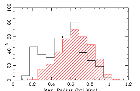
Figure 1: Distribution of maximum APM cluster radius used to define the cluster shape parameters for $R_{\delta}=0.24$ (thick line) and $R_{\delta}=0.36$ (hatched). Only the 405 APM clusters with no significant substructure are used (see section 3.4)

3.2 Testing the Performance of our Method

The two procedures to determine cluster shape parameters may be biased by the unavoidable presence of foreground and background galaxies projected on the clusters, and may also have systematic biases due to the methods themselves. In this section we investigate the robustness of the two methods in recovering the true projected cluster shape in the presence of discreteness effects and the galaxy background.

To this end we generate a large number of mock clusters, resembling in appearance dynamically relaxed structures; ie., having no substructure and King-like surface brightness profiles:

$$\Sigma(r)\propto\left[1+\left(\frac{r}{r_{c}}\right)^{2}\right]^{-\alpha}\;\;,$$ (5)

where $r_{c}$ is the cluster core radius and $\alpha$ is the slope parameter. Different values of the slope and core radius have been found in different studies, spanning the range $0.6\raise-2.0pt\hbox{\hbox to0.0pt{\hbox{$\sim$}\hss}\raise 5.0pt\hbox{$<$}\ }\alpha\raise-2.0pt\hbox{\hbox to0.0pt{\hbox{$\sim$}\hss}\raise 5.0pt\hbox{$<$}\ }1$ and $0.1\raise-2.0pt\hbox{\hbox to0.0pt{\hbox{$\sim$}\hss}\raise 5.0pt\hbox{$<$}\ }r_{c}\raise-2.0pt\hbox{\hbox to0.0pt{\hbox{$\sim$}\hss}\raise 5.0pt\hbox{$<$}\ }0.25$ $h^{-1}$ Mpc (cf. Bachall & Lubin 1993; Girardi et al. 1995; Girardi et al. 1998). The latter study, using the ENACS optical sample of Abell clusters, found a median value of $\alpha\simeq 0.65_{-0.07}^{+0.05}$. We create our mock clusters by randomly generating galaxies having $\alpha=0.65$, $r_{c}=0.18$ and input ellipticities of our choice. We have tested that small variations of these parameters do not alter significantly our results.

The expected global background at each cluster can be estimated by:

$$N_{back}={\rm d}\Omega_{i}\int_{0}^{z_{max}}\langle\rho(z)\rangle z^{2}dz$$ (6)

where $z_{max}$ is the maximum redshift of galaxies in the APM catalogue ($\sim 0.3$), ${\rm d}\Omega_{i}$ is the solid angle covered by the cluster, given by ${\rm d}\Omega_{i}=2\pi(1-cos\theta_{i})$ for a cluster with angular radius $\theta_{i}$, and $\langle\rho(z)\rangle$ is the mean APM galaxy density at redshift $z$, obtained by integrating the APM galaxy luminosity function, $\Phi(M,z)$, allowing for evolution (Maddox, Efstathiou & Sutherland 1996):

$$\langle\rho(z)\rangle=\int^{M_{max}}_{M_{min}(z)}\Phi(M,z)dM\;,$$ (7)

with $M_{min}(z)$ the minimum absolute magnitude that a galaxy at a redshift $z$ can have and still be included in the APM catalogue, limited in apparent magnitude by $m_{lim}=20.5$, ie; $M_{min}(z)=m_{lim}-42.38-5\log z+5\log h-3z\;\;.$ The points in figure 2 show the number of APM galaxies counted within a radius of 1.2 $h^{-1}$ Mpc from each cluster center, and the line shows the predicted global background, $N_{back}$. Both are decreasing functions of distance due to the apparent magnitude limit of the APM galaxy catalogue.

Figure 2: The APM cluster richness (number of galaxies within a $1.2\;h^{-1}$ Mpc radius) and the expected number of background galaxies as a function of distance.

For our Monte-Carlo simulations we generate a random galaxy background, with number density given from eq.(6), in a circular area of radius equal to the semi-major axis of the ellipse. As an example we plot in figure 3 the smooth galaxy density distribution of two mock clusters with $\epsilon_{th}=0.5$ at distances $r=200\;h^{-1}$ Mpc and $380\;h^{-1}$ Mpc, respectively and having the typical APM cluster richness at that distance. As expected the random background tends to sphericalize the clusters.

The question that we want to answer now is: “Given an input cluster ellipticity what is the most probable measured ellipticity recovered by our methods?” We present a case study of the mock cluster at a distance of $200\;h^{-1}$ Mpc, having a range of input projected ellipticities of width 0.1. We generate 100 Monte-Carlo realizations of the cluster for each input ellipticity. In the left panel of figure 4 we present the measured mean ellipticities, and their scatter for both methods in the absence of a background galaxy distribution. Both methods give similar results, with the first method recovering (for $\epsilon_{th}\raise-2.0pt\hbox{\hbox to0.0pt{\hbox{$\sim$}\hss}\raise 5.0pt\hbox{$>$}\ }0.1$) exactly the input (correct) ellipticities.

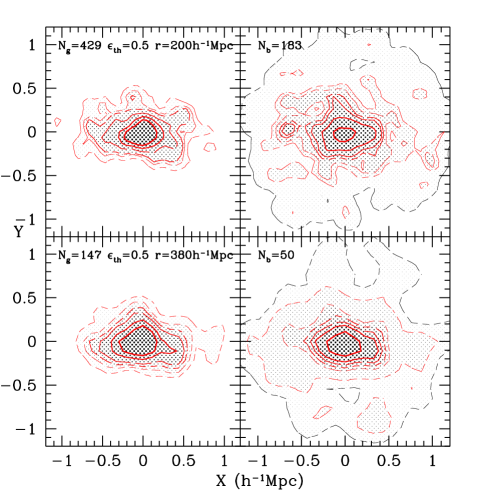
Figure 3: The density contours for two mock clusters using a King-like profile and input ellipticity $\epsilon_{th}=0.5$.

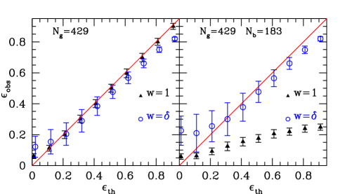
Figure 4: Performance of our shape determination method for a simulated cluster at $200\;h^{-1}$ Mpc containing 429 galaxies, by comparing the input and measured ellipticities, using either $w=1$ or $w=\delta$ weights. The left panel presents the case for no background galaxy contamination. The right panel presents the more realistic situation in which we superimpose a random background galaxy distribution according to eq.(6).

The right panel of figure 4 presents the results for the same mock cluster but now we include the random background galaxy distribution, appropriate for the distance of the cluster. The first method breaks down and severely underestimates the input ellipticities for $\epsilon>0.1$. It is evident that only the $w=\delta$ method performs relatively well in the presence of the galaxy background and from now on we will be using only this method.

Performing many tests with mock clusters at different distances, we conclude that the grid method has a variable performance as a function of distance, tending to increasingly underestimate the ellipticity of elongated clusters as a function of distance (by about 0.1-0.15). For clusters with $\epsilon_{th}\raise-2.0pt\hbox{\hbox to0.0pt{\hbox{$\sim$}\hss}\raise 5.0pt\hbox{$<$}\ }0.2-0.25$ the relation between input and recovered ellipticity is non-monotonic, which means it is not possible to correct the measured ellipticities of APM clusters for the systematic biases which are evident in the right panel of figure 4. These numerical tests have served mostly to choose between the two shape determination procedures, rather than to derive a robust ellipticity correction procedure.

3.3 Correcting systematic ellipticity biases

Since cluster ellipticities cannot be corrected on an individual basis we must apply a statistical correction to the ellipticity distribution to deal with all the above mentioned systematic effects. In order to do this, we need to answer a slightly different question from the one we posed previously. The relevant question is: “What is the distribution of input (correct) ellipticities from which a measured ellipticity can be obtained?” For each APM cluster with measured ellipticity, $\epsilon_{obs}$, we generate 50 mock Monte-Carlo clusters for each ellipticity bin of width 0.05, spanning the whole range $\epsilon_{th}\in(0,1)$. These mock clusters, 1000 in total, have the same number of cluster and background galaxies and are placed at the same distance as the one observed. We measure the ellipticity of the mock clusters, $\epsilon_{mock}$, and derive its distribution function per each input ($\epsilon_{th}$) ellipticity bin. We then measure, assuming Gaussian statistics, how many standard deviations the original APM cluster measured ellipticity ($\epsilon_{obs}$) differs from the derived mean mock value, $\langle\epsilon_{mock}\rangle$, and assign to the corresponding input ellipticity ($\epsilon_{th}$) bin the resulting probability. Therefore, for each input ($\epsilon_{th}$) ellipticity bin $i$ we estimate the probability of being the correct ellipticity from which the APM measured one could have resulted; ie,

$$P^{i}(\epsilon_{th})=1-P(z_{i})$$ (8)

where $z_{i}=|\epsilon_{obs}-\langle\epsilon^{i}_{mock}\rangle|/\sigma_{i}$. If for example, for some bin $i$, the value of $|\epsilon_{obs}-\langle\epsilon^{i}_{mock}\rangle|=4\sigma_{i}$ then $z_{i}=4$, $P(z_{i})\simeq 1$ and thus the probability of $\epsilon^{i}_{th}$ being the correct APM cluster ellipticity is $P^{i}\simeq 0$. Doing so for all bins we derive the full probability distribution function of input (correct) ellipticities, $P(\epsilon_{th})$, from which our measured APM cluster ellipticity could have resulted. For each APM cluster we have therefore generated in total 1000 mock clusters (50 per $\epsilon_{th}$ bin) which provide an estimate $P(\epsilon_{th})$ for that cluster. The final step in estimating the corrected cluster ellipticity distribution is to add the contribution from each cluster by randomly sampling its $P(\epsilon_{th})$ $N$ times (we have used $N=20$). We stress that the correction procedure is applied separately to each individual APM cluster which means that the corrections take into account the variations in performance of our shape determination method as a function of different cluster richness and distance.

As an illustrative example we plot in figure 5 the $P(\epsilon_{th})$ distribution for three distant clusters ($r\simeq 320$ $h^{-1}$ Mpc) with $\epsilon_{obs}\simeq 0.2,0.5$ and 0.7 respectively. For the $\epsilon_{obs}=0.2$ case the $P(\epsilon_{th})$ is quite flat in the range $0\raise-2.0pt\hbox{\hbox to0.0pt{\hbox{$\sim$}\hss}\raise 5.0pt\hbox{$<$}\ }\epsilon_{th}\raise-2.0pt\hbox{\hbox to0.0pt{\hbox{$\sim$}\hss}\raise 5.0pt\hbox{$<$}\ }0.2$, having a long tail up to $\epsilon_{th}\simeq 0.6$. The $\epsilon_{obs}=0.5$ case has a $P(\epsilon_{th})$ distribution that peaks at $\sim 0.65$ but also has a significant contribution from lower ellipticities. Finally for the $\epsilon_{obs}=0.7$ case the most probable value of $\epsilon_{th}$ is $\sim 0.9$. These facts serve to show that in order to produce the correct apparent cluster ellipticity distribution it is essential to use a statistical procedure and sample each $P(\epsilon_{th})$ distribution adequately.

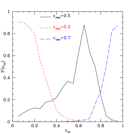
Figure 5: The probability functions for some characteristic measured ellipticities ($\epsilon_{obs}=0.2,0.5$ and 0.7) of three APM clusters containing $\simeq 140$ galaxies and at a distance of $\sim 320$ $h^{-1}$ Mpc.

3.4 Substructure of APM clusters

The correction procedure of the ellipticity distribution is based on the assumption that the clusters under study have a smooth King-like density profile. Therefore we need to exclude from our sample clusters that exhibit evidence of significant substructure. The number of clusters with substructure, expected to be undergoing dynamical evolution, is an unsettled issue but of great importance since it provides information of the mean density of the universe (cf. Richstone et al. 1992; Dutta 1995; Buote 1998; Thomas et al. 1998). In an $\Omega=1$ universe, clusters continue to form even today and therefore one expects more substructure than in a low $\Omega$ universe. Identifying real sub-clumps in clusters is a difficult problem in general, since one has to work either in two-dimensions, in which projection effects can significantly affect the visual structure of clusters, or in redshift space, where distortions due to knowledge of only the radial velocity component can again distort the true pattern. Several studies indicate that at least $\sim 30\%-50\%$ (cf. West 1994 and references therein; Jones & Forman 1999) of rich clusters have strong substructure in their gas or galaxy distribution within $\simeq 1\;h^{-1}$ Mpc of the cluster center.

Here, we present the main steps of our substructure identification method, the full details and results will be presented in a forthcoming paper. We work on the smoothed density field, as described in section 3.1. For each overdensity threshold, estimated for $R_{\delta}=0.12,0.24$ and 0.36 $h^{-1}$ Mpc, we select all grid-cells with overdensities above the specific threshold. We then connect all cells that have common borders to create multiple clumps. In all cases we accept only clumps that are within $\simeq 0.75\;h^{-1}$ Mpc of the highest cluster peak; we have found this scale to be optimal for reliable substructure identification by validating our methods and results using ROSAT data for a subsample of 22 clusters (Kolokotronis et al. 2000), which also corresponds to the counting radius used in the APM cluster finding algorithm (cf. Dalton et al. 1997).

Investigation of the number and size of these clumps as a function of overdensity threshold, provides the following categorisation:

• No substructure (69 clusters): Clusters with one clump in all overdensity levels.

• Weak substructure (336 clusters): Multiple clumps only at the lowest overdensity level or at the highest two overdensity levels but where the second in size clump is $<20\%$ of the total cluster size (cf. Richstone et al. 1992).

• Strong substructure (498 clusters): Multiple clumps where the second in size clump is $\raise-2.0pt\hbox{\hbox to0.0pt{\hbox{$\sim$}\hss}\raise 5.0pt\hbox{$>$}\ }20\%$ of the total cluster size.

We have investigated the robustness of our substructure characterisation procedure, as a function of different $R_{\delta}$, and found only small variations, consisting mainly of a movement of APM clusters between the “no” and “weak” substructure categories. We have also verified that due to the random galaxy background, coupled with discreteness effects, it is common to find “weak” substructure even in our mock clusters which by construction have no substructure. Therefore we exclude from our shape determination analysis only those APM clusters that were found to have “strong” substructure.

4 True Cluster Shapes

In order to find the intrinsic ellipticity distribution assuming that clusters are all oblate or prolate spheroids, we use a standard method based on the kernel estimator.

4.1 Kernel estimator

General reviews of kernel estimators are given by Silverman (1986) and Scott (1992) but the applications to the astronomical data are given by Vio et al. 1994, Tremblay & Merritt (1995) and Ryden (1996). Here we review the basic steps of the Kernel method, following the notation of Ryden (1996). For each estimated ellipticity $\epsilon$, we estimate the axial ratio, $q=\left(\frac{1-\epsilon}{1+\epsilon}\right)^{1/2}$. Given the sample of axis ratios $q_{1},q_{2},....,q_{N}$ for $N$ clusters, the kernel estimate of the frequency distribution is defined as:

$$\hat{f}(q)=\frac{1}{Nh}\sum_{i}^{N}\ K\left(\frac{q-q_{i}}{h}\right)\;\;,$$ (9)

where $K(t)$ is the kernel function, defined so that

$$\int_{-\infty}^{+\infty}\ K(t){\rm d}t=1\;\;,$$ (10)

and $h$ is the “kernel width” which determines the balance between smoothing and noise in the estimated distribution. In general the value of $h$ is chosen so that the expected value of the integrated mean square error between the true, $f(q)$, and estimated, $\hat{f}(q)$, distributions, $\int_{-\infty}^{+\infty}\left[\hat{f}_{K}(x)-f(x)\right]^{2}{\rm d}x$, is minimised (cf. Vio et al. 1994; Tremblay & Merritt 1995). In this work we estimate the $h$ using a very common approach presented by Silverman (1986), Vio et al. (1994) and Ryden (1996) in which:

$$h=0.9AN^{-1/5}$$ (11)

where $N$ is the number of the clusters and $A=\min(\sigma,Q_{4}/1.34)$, with $Q_{4}$ the interquartile range. There are three common choices for the kernel function $K(t)$ which have quadratic, quartic and Gaussian forms (cf. Tremblay & Merritt 1995). Many studies have shown that the choice of a kernel function does not in general affect the estimates, and they differ trivially in their asymptotic efficiencies. We have chosen a Gaussian kernel:

$$K(t)=\frac{1}{\sqrt{2\pi}}e^{-t^{2}/2}\;\;.$$ (12)

In order to obtain physically acceptable results with $\hat{f}(q)=0$ for $q<0$ and $q>1$, we apply reflective boundary conditions which means that the Gaussian kernel is replaced with:

$$K(q,q_{i},h)=K\!\!\left(\frac{q-q_{i}}{h}\right)+K\!\!\left(\frac{q+q_{i}}{h}\right)+K\!\!\left(\frac{2-q-q_{i}}{h}\right)$$ (13)

This also ensures the correct normalization, $\int_{0}^{1}\hat{f}(q){\rm d}q=1$. For a discussion of reflective boundary conditions see Silverman (1986) and Ryden (1996).

Figure 6: In the top panel the crosses show the uncorrected distribution of apparent axial ratios for the complete sample of 903 APM clusters with the solid line being the smooth distribution from the nonparametric kernel estimator. The open circles correspond to the distribution of the 405 APM clusters with no significant substructure. In the lower panel we present the corrected axial ratio distribution for the later clusters.

The crosses in figure 6 show the projected axial ratio distributions with the Poisson 1$\sigma$ error bars and the solid lines show the kernel estimate $\hat{f}$ with width $h=0.075$. In the top panel we present our results for the uncorrected distribution of all 903 APM clusters; which can crudely be fitted by a Gaussian with $\langle q\rangle\simeq 0.65$ and standard deviation $\simeq 0.15$. In the bottom panel we present the corrected distribution using the 405 APM clusters free of significant subclustering. It is obvious that the two distributions are significantly different, with the peak of the corrected distribution having moved to lower $q$’s but with an extended contribution of apparently quasi-spherical objects.

4.2 Inversion method

The relation between the apparent and intrinsic axial ratios, is described by a set of integral equations first investigated by Hubble (1926). These are based on the assumptions that the orientations are random with respect to the line of sight, and that the intrinsic shapes can be approximated by either oblate or prolate spheroids. There is no physical justification for the restriction to oblate or prolate but it greatly simplifies the inversion problem. Furthermore, if the intrinsic shape of clusters is triaxial or a mixture of the two spheroidal populations then there is no unique inversion (PBF). Writing the intrinsic axial ratios as $\beta$ and the estimated distribution function as $\hat{N}_{o}(\beta)$ for oblate spheroids, and $\hat{N}_{p}(\beta)$ for prolate spheroids then the corresponding distribution of apparent axial ratios is given for the oblate case by:

$$\hat{f}(q)=q\int_{0}^{q}\frac{\hat{N}_{\circ}(\beta){\rm d}\beta}{(1-q^{2})^{1/2}(q^{2}-\beta^{2})^{1/2}}$$ (14)

and for the prolate case by:

$$\hat{f}(q)=\frac{1}{q^{2}}\int_{0}^{q}\frac{\beta^{2}\hat{N}_{p}(\beta){\rm d}\beta}{(1-q^{2})^{1/2}(q^{2}-\beta^{2})^{1/2}}\;\;.$$ (15)

Inverting equations (eq.14) and (eq.15) gives us the distribution of real axial ratios as a function of the measured distribution:

$$\hat{N}_{o}(\beta)=\frac{2\beta(1-\beta^{2})^{1/2}}{\pi}\int_{0}^{\beta}\ \frac{\rm d}{{\rm d}q}\left(\frac{\hat{f}}{q}\right)\frac{{\rm d}q}{(\beta^{2}-q^{2})^{1/2}}$$ (16)

and

$$\hat{N}_{p}(\beta)=\frac{2(1-\beta^{2})^{1/2}}{\pi\beta}\int_{0}^{\beta}\ \frac{\rm d}{{\rm d}q}(q^{2}\hat{f})\frac{{\rm d}q}{(\beta^{2}-q^{2})^{1/2}}\;\;.$$ (17)

with $\hat{f}(0)=0$. In order for $\hat{N}_{p}(\beta)$ and $\hat{N}_{o}(\beta)$ to be physically meaningful they should be positive for all $\beta$’s. Following Ryden (1996), we numerically integrate eq.(16) and eq.(17) allowing $\hat{N}_{p}(\beta)$ and $\hat{N}_{o}(\beta)$ to take any value. If the inverted distribution of axial ratios has significantly negative values, a fact which is unphysical, then this can be viewed as a strong indication that the particular spheroidal model is unacceptable.

In figure 7 we present the uncorrected and corrected intrinsic axial ratio distributions. The uncorrected distribution for both spheroidal models takes negative values; over the range $\beta\raise-2.0pt\hbox{\hbox to0.0pt{\hbox{$\sim$}\hss}\raise 5.0pt\hbox{$>$}\ }0.7$ for the oblate case, and $\beta\raise-2.0pt\hbox{\hbox to0.0pt{\hbox{$\sim$}\hss}\raise 5.0pt\hbox{$>$}\ }0.8$ for the prolate case. Using the corrected apparent axial-ratio distributions $\hat{f}(q)$, the oblate model produces negative values of $N$ for $\beta\raise-2.0pt\hbox{\hbox to0.0pt{\hbox{$\sim$}\hss}\raise 5.0pt\hbox{$>$}\ }0.5$ and $\beta\raise-2.0pt\hbox{\hbox to0.0pt{\hbox{$\sim$}\hss}\raise 5.0pt\hbox{$<$}\ }0.2$, but the prolate one provides a distribution of intrinsic axial ratios that is positive over the whole $\beta$ range.

Figure 7: The distribution of intrinsic APM cluster axial ratios and its $1\sigma$ range, for the corrected and uncorrected samples, assuming that clusters are either oblate or prolate spheroids.

This suggests that the APM cluster shapes are better represented by that of prolate spheroids rather than oblate, which is in agreement with PBF and Cooray (1999). However, it is probably not realistic to assume a population of pure oblate or prolate spheroids but rather of triaxial ellipsoids, in which case the inversion procedure is not unique (see PBF). Nevertheless, our results strongly suggest that cluster prolateness should be a dominant feature.

5 Conclusions

We have measured the projected ellipticities of all APM clusters using moments either of the individual galaxy distribution or of the smoothed galaxy distribution above some overdensity threshold. We have performed large sets of Monte Carlo simulations in order to test the statistical robustness of the two procedures, and conclude that the first method is strongly affected by the presence of background galaxies whereas the second method better recovers the underline true cluster projected ellipticity.

We devised a statistical Monte-Carlo procedure to correct the distribution of cluster ellipticities for the systematic errors introduced by discreteness effects, background galaxies and the method itself. The procedure involves estimating first the probability distribution of the true projected ellipticity for each APM cluster, and then random sampling this probability distribution to estimate the cluster’s contribution to the corrected overall projected cluster ellipticity distribution. This method works well only for clusters that appear relaxed, with no significant substructure. ‘Therefore we have excluded, from our final cluster sample which contains 405 clusters, all the APM clusters that show evidence of significant substructure. Prior to the exclusion of these clusters the uncorrected axial ratio distribution of the whole APM cluster sample can be crudely approximated by a Gaussian with a mean of $\simeq 0.65$ and a standard deviation of $\simeq 0.15$. The corrected apparent axial-ratio distribution is significantly different showing a bump at $q\simeq 0.46$ and having a significant contribution from apparently quasi-spherical systems.

Using the nonparametric kernel procedure we obtain a smooth estimate of the apparent APM cluster axial-ratio distribution. We assume that the APM clusters are a homogeneous population of either oblate or prolate spheroids and numerically invert the apparent distribution to obtain the intrinsic distribution. The most acceptable model is provided by that of prolate spheroids. This result supports the view by which clusters form by accretion of smaller units along the large-scale structure (filament) in which they are embedded (cf. West 1994; West, Jones & Forman 1995). Such an accretion process would happen preferentially along the cluster major axis, which is typically aligned with the nearest cluster neighbour (cf. Bingelli 1982; Plionis 1994 and references therein).

Since cluster shapes and substructure are sensitive cosmological probes (Evrard et al. 1993), we plan to investigate these issues further using APM clusters and compare our results with theoretical expectations, provided by high-resolution N-body simulations of different cosmological models (cf. Thomas et al.1998).

References

- [] Bahcall, N., A., & Lubin, L. M., 1993, ApJ, 415, L17
- [] Bingelli B., 1982, AA, 250, 432
- [] Buote, D. A., 1998, MNRAS, 293, 381
- [] Buote, D. A., Tsai, J. C., 1995a, ApJ, 439,29
- [] Buote, D. A., Canizares, C. R., 1996, ApJ, 457, 565
- [] Canizares, C. R. & Buote, D.A., 1997, ASCA proceedings on “Xray Imaging & Spectroscopy of Cosmic Hot Plasmas”, Eds. F.Makino & K.Mitsuda.
- [] Carter, D. & Metcalfe, J., 1980, MNRAS, 191, 325
- [] Coorey, R.A., 1999, astro-ph/9905094
- [] Dalton, G. B., Maddox S. J., Sutherland W. J., Efstathiou G. 1997, MNRAS, 289 , 263
- [] Di Fazio, A. & Flin, P., 1988, AA, 200, 5
- [] Dutta, S., 1995, MNRAS, 276 , 1109
- [] Efstathiou, G., Frenk, C.S., White, S.D., Davis M., 1988, MNRAS, 235, 715
- [] Evrard, A. E., Mohr, J.J. , Fabricant, D.G., Geller, M. J., 1993, ApJ, 419, L9
- [] Fall, M. & Frenk, C. S., 1983, ApJ, 88, 1626
- [] Frenk, C.S., White, S.D., Efstathiou, G., Loveday, J., 1988, ApJ, 327, 507
- [] Girardi, M., Biviano A., Giuricin G., Mardirossian F., Mezzetti M., 1995, ApJ, 438, 527
- [] Girardi, M., Giuricin G., Mardirossian, F., Mezzetti M., Boschin W., 1998, ApJ, 505, 74
- [] Jones, C. & Forman, W., 1999, ApJ, 511, 65
- [] Lambas, D., Maddox, S., & Loveday, J., 1992, MNRAS, 258, 404
- [] Maddox S.J. , Sutherland W.J., Efstathiou G., Loveday, J. 1990a, MNRAS, 243, 692
- [] Maddox S.J., Efstathiou G., Sutherland W.J., 1990b, MNRAS, 246, 433
- [] Maddox S.J. , Sutherland W.J., Efstathiou G., Loveday, J., Peterson, B.A., 1990c, MNRAS, 247, 1P
- [] Maddox S. J., Efstathiou G., Sutherland W. J., 1996, MNRAS, 283, 1227
- [] McMillan S. L. W., Kowalski M. P., Ulmer M. P., 1989, ApJ, 70, 723
- [] Mohr, J.J., Evrard, A.E., Fabricant, D.G., Geller, M.J., 1995, ApJ, 447, 8
- [] Plionis M., 1994, ApJS., 95, 401
- [] Plionis M., Barrow J.D., Frenk, C.S., 1991, MNRAS, 249, 662
- [] Richstone, D., Loeb, A., Turner, E.L., 1992, ApJ, 393, 477
- [] Ryden S.B., 1996, ApJ, 461, 146
- [] Sandage, A., Binggeli, G., Tammann, G. A., 1985, AJ, 90, 1759
- [] Scott, D. W., 1992, Multivariate Density Estimation for Statistics and Data Analysis (New York: Chapman & Hall)
- [] Silverman, B. W., 1986, Density Estimation for Statistics and Data Analysis (New York: Chapman & Hall)
- [] Struble. M. F., & Ftaclas C., 1994, AJ, 108, p1-23
- [] De Theije, P.A.M., Katgert, P. & van Kampen E., 1995, MNRAS, 273, 30
- [] Thomas, P. A., et al, 1998, MNRAS, 296, 1061
- [] Tremblay, B., & Merrit, D., 1995, AJ, 110, 1039
- [] Ulmer, McMillan S. L. W., Kowalski M. P., 1989, ApJ, 338, 711
- [] Valdarnini, R., Ghizzardi, S., Bonometto, S., 1999, NewA, 4, 71
- [] Vio, R., Fasano, G., Lazzarin, M., Lessi, O., 1994, AA, 289, 640
- [] West, M. J., 1994, MNRAS, 268, 79
- [] West, M. J., Jones C., Forman W., 1995, ApJ, 451, L5