The Evolution of ⁴He and LiBeB

Abstract

Our understanding of the evolution of ⁴He and ⁷Li depends critically on the available data for these two elements at low metallicity. In particular, the degree to which there is a slope in an abundance vs metallicity regression can help determine the evolution of He, C, N, and O in dwarf galaxies in the case of ⁴He, and cosmic-ray induced nucleosynthesis of LiBeB in our own galaxy in the case of ⁷Li. Recent data and their implications will be discussed.

UMN–TH–1840/00

TPI–MINN–00/06

January 2000

Theoretical Physics Institute, School of Physics and Astronomy, University of Minnesota, Minneapolis MN 55455, USA

1. Introduction

There is a relatively large set of data available on the big bang nucleosynthesis (BBN) element isotopes of ⁴He and ⁷Li at low metallicity. It is common, particularly in the case of ⁴He, to perform a linear regression on the data with respect to some metallicity tracer such as O/H or Fe/H. The intercept of such a regression can be directly related to the primordial abundance of that isotope, and the slope of the regression offers important clues to the nature of its chemical evolution. While one can not necessarily justify a linear relation from first principles, generally due to the quality of the data at low metallicity, such an approximation is acceptable. In fact, using the currently available ⁴He and ⁷Li data, it is easy to show that a linear regression is significantly better than a weighted mean, yet more complicated fits using additional parameters generally do not yield a statistically significant improvement in the fit.

Our inferences of the primordial abundances and evolution of the light elements are clearly tied to the quality of the data and our understanding of the systematic uncertainties in the derived abundances. Evolution is one the effects which is responsible for systematic uncertainties. In the case of ⁴He, the environment of the HII system is not pristine and includes non-primordial ⁴He. In addition, the true elemental abundances of ⁴He may be clouded due to effects such as underlying stellar absorption, collisional excitation, or flourecence. In the case of ⁷Li, abundances are contaminated by the non-primordial contribution of ⁷Li from galactic cosmic-ray nucleosynthesis (GCRN) and uncertainties concerning the degree of stellar depletion of ⁷Li in pop II, halo stars.

2. ⁴He

The ⁴He abundance has been determined from observations of HeII $\rightarrow$ HeI recombination lines in a large sample of extragalactic HII regions (Pagel et al. 1992; Skillman & Kennicutt 1993; Skillman et al. 1994; Izotov, Thuan, & Lipovetsky 1994,1997; Izotov & Thuan 1998). Since ⁴He is produced in stars along with heavier elements such as Oxygen, it is expected that the primordial abundance of ⁴He can be determined from the intercept of the correlation between $Y$ and O/H, namely $Y_{p}=Y({\rm O/H}\to 0)$. A detailed analysis of the combined data (Olive, Skillman, & Steigman 1997; Fields & Olive 1998) found an intercept corresponding to a primordial abundance

$$Y_{p}=0.238\pm 0.002\pm 0.005$$ (1)

The first uncertainty is purely statistical and the second uncertainty is an estimate of the systematic uncertainty in the primordial abundance determination. The helium abundance used in this analysis was determined using electron densities $n$ obtained from SII data. Izotov, Thuan, & Lipovetsky (1994,1997) and Izotov & Thuan (1998) proposed a method based on several He emission lines to “self-consistently” determine the electron density. This method yields a higher primordial value

$$Y_{p}=0.244\pm 0.002\pm 0.005$$ (2)

Our interpretation of the evolution of ⁴He depends heavily on the slope of the ⁴He abundance with respect to a tracer element such as O/H and/or N/H. While models of chemical evolution tend to give relatively low slopes ($\Delta Y/\Delta(O/H)\sim 20-60$), the He data based on SII densities gives a much larger slope ($\Delta Y/\Delta(O/H)\sim 110\pm 25$), whereas the self-consistent method gives ($\Delta Y/\Delta(O/H)\sim 47\pm 26$). The model calculations (Fields & Olive 1998, and references therein) depend crucially on the assumed yields of N in the AGB phase and on assumptions concerning hot-bottom burning. Many of the models attempting to reproduce the higher He slopes also rely on significant amounts of outflow in these dwarf galaxies.

As can be ascertained from the brief discussion above, the method of analysis has a huge impact on both the determination of the primordial ⁴He abundance and the slope of the He vs O/H regression. Therefore, rather than discuss specific chemical evolution models in detail here, I will discuss some of the key sources of the uncertainties in the He abundance determinations and prospects for improvement.

The He abundance is always quoted relative to H, e.g., He line strengthes are measured relative to $H\beta$. The H data must first be corrected for underlying absorption and reddening. Beginning with an observed line flux $F(\lambda)$, and an equivalent width $W(\lambda)$, we can parameterize the correction for underlying stellar absorption as

$$X_{A}(\lambda)=F(\lambda)({W(\lambda)+a)\over W(\lambda)})$$ (3)

The parameter $a$ is expected to be relatively insensitive to wavelength. A reddening correction is applied to determine the intrinsic line intensity $I(\lambda)$ relative to $H\beta$

$$X_{R}(\lambda)={I(\lambda)\over I(H\beta)}={X_{A}(\lambda)\over X_{A}(H\beta)}10^{f(\lambda)C(H\beta)}$$ (4)

where $f(\lambda)$ represents an assumed universal reddening law and $C(H\beta$) is the correction factor to be determined. By comparing $X_{R}(\lambda)$ to theoretical values, $X_{T}(\lambda)$, we determine the parameters $a$ and $C(H\beta)$ self consistently (Olive & Skillman, 2000), and run a Monte Carlo over the input data to test the robustness of the solution and to determine the systematic uncertainty associated with these corrections.

In Figure 1 (from Olive & Skillman 2000), I show the result of such a Monte-Carlo based on synthetic data with an assumed correction of 2 Å for underlying absorption and a value for $C(H\beta)=0.1$. The synthetic data were assumed to have an intrinsic 2% uncertainty. While the mean value of the Monte-Carlo results very accurately reproduces the input parameters, the spread in the values for $a$ and $C(H\beta)$ are generally a factor of 2 larger than one would have derived from the direct solution due to the covarience in $a$ and $C(H\beta)$.

Figure 1.: A Monte Carlo determination of the underlying absorption $a$ (in Å ), and reddening parameter $C(H\beta)$, based on synthetic data.

The uncertainties found for $H\beta$ must next be propagated into the analysis for ⁴He, for which we follow an analogous procedure to that described above (Olive & Skillman 2000). We again start with a set of observed quantities: line intensities $I(\lambda)$ which include the reddening correction previously determined along with its associated uncertainty which includes the uncertainties in $C(H\beta)$; the equivalent width $W(\lambda)$; and temperature $t$. The Helium line intensities are scaled to $H\beta$ and the singly ionized helium abundance is given by

$$y^{+}(\lambda)={I(\lambda)\over I(H\beta)}{E(H\beta)\over E(\lambda)}({W(\lambda)+a^{\prime}\over W(\lambda)}){1\over(1+\gamma)}{1\over f(\tau)}$$ (5)

where $E(\lambda)/E(H\beta)$ is the theoretical emissivity scaled to $H\beta$. The expression (5) also contains a correction factor for underlying stellar absorption, parameterized now by $a^{\prime}$, a density dependent collisional correction factor, $(1+\gamma)^{-1}$, and a flourecence correction which depends on the optical depth $\tau$. Thus $y^{+}$ implicitly depends on 3 unknowns, the electron density, $n$, $a^{\prime}$, and $\tau$.

One can use 3-6 lines to determine the weighted average helium abundance, $\bar{y}$. From ${\bar{y}}$, we can calculate the $\chi^{2}$ deviation from the average, and minimize $\chi^{2}$, to determine $n,a^{\prime}$, and $\tau$. Uncertainties in the output parameters are also determined.

This procedure differs somewhat from that proposed by ITL, in that the $\chi^{2}$ above is based on a straight weighted average, where as ITL minimize the difference of a ratio of He abundances (to one wavelength, say $\lambda$4471) to the theoretical ratio. When the reference line is particularly sensitive to a systematic effect such as underlying stellar absorption, this uncertainty propagates to all lines this way. In our case, the individual uncertainties in the line strengths are kept separate.

Finally, as in the case for the hydrogen lines, we have performed a Monte-Carlo simulation of the data to test the robustness of the solution for $n,a^{\prime}$, and $\tau$ (Olive & Skillman 2000). In Figure 2, I show the result of a single case based on the data of Izatov and Thuan (1998) for SBS1159+545. Here, the helium abundance and density solutions are displayed. The vertical and horizontal lines show the position of the IT solution. The circle shows the position of the our solution to the minimization, and the square shows the position of the mean of the Monte-Carlo distribution. The spread shown here is significantly greater than the uncertainty quoted by IT.

Figure 2.: A Monte Carlo determination of the helium abundance and electron density (in cm^-3). Solutions for $a^{\prime}$ and $\tau$ are not shown here.

3. ⁷Li

The population II abundance of ⁷Li has been determined by observations of over 100 hot, halo stars, and is found to have a very nearly uniform abundance (Spite & Spite 1982). For stars with a surface temperature $T>5500$ K and a metallicity less than about 1/20th solar, the abundances show little or no dispersion beyond that which is consistent with the errors of individual measurements. The Li data from Bonifacio & Molaro (1997) indicate a mean ⁷Li abundance of

$${\rm Li/H=(1.6\pm 0.1)\times 10^{-10}}$$ (6)

The small error is statistical and is due to the large number of stars in which ⁷Li has been observed.

There is, however, an important source of systematic error due to the possibility that Li has been depleted in these stars, though the lack of dispersion in the Li data limits the amount of depletion. In fact, as discussed by Sean Ryan (these proceedings, and Ryan, Norris, & Beers, 1999, hereafter RNB) a small observed slope in Li vs Fe and the tiny dispersion about that correlation indicates that depletion is negligible in these stars. Furthermore, the slope may indicate a lower abundance of Li than that in (6).

For reference, the weighted mean of the ⁷Li abundance in the RNB sample is [Li] = 2.12 ([Li] = $\log$ ⁷Li/H + 12). It is common to test for the presence of a slope in the Li data by fitting a regression of the form [Li] = $\alpha+\beta$ [Fe/H]. The RNB data indicate a rather large slope, $\beta=0.07-0.16$ and hence a downward shift in the “primordial” lithium abundance $\Delta$[Li] = $-0.20--0.09$. Models of galactic evolution which predict a small slope for [Li] vs. [Fe/H], can produce a value for $\beta$ in the range 0.04 – 0.07 (Ryan et al. 2000). Of course, if we would like to extract the primordial ⁷Li abundance, we must examine the linear (rather than log) regressions. For Li/H = $a^{\prime}+b^{\prime}$Fe/Fe_⊙, we find $a^{\prime}=1-1.2\times 10^{-10}$ and $b^{\prime}=40-120\times 10^{-10}$. A similar result is found fitting Li vs O. Overall, when the regression based on the data and other systematic effects are taken into account a best value for Li/H was found to be (Ryan et al. 2000)

$${\rm Li/H=1.23\times 10^{-10}}$$ (7)

with a plausible range between 0.9 – 1.9 $\times 10^{-10}$.

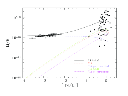
Figure 3.: Contributions to the total predicted lithium abundance from the adopted GCE model of Fields & Olive (1999a,b), compared with low metallicity stars (RNB) and a sample of high metallicity stars. The solid curve is the sum of all components.

Figure 3 shows the different Li components for a model with (⁷Li/H)${}_{p}=1.23\times 10^{-10}$. The linear slope produced by the model is $b^{\prime}=65\times 10^{-10}$, and is independent of the input primordial value (unlike the log slope given above). The model (discussed in detail in Fields & Olive, 1999a,b and Fields et al. 2000) includes in addition to primordial ⁷Li, lithium produced in galactic cosmic ray nucleosynthesis, (primarily $\alpha+\alpha$ fusion) in addition to ⁷Li produced by the $\nu$-process during type II supernovae. As one can see, these processes are not sufficient to reproduce the population I abundance of ⁷Li, and additional production sources are needed (see e.g. Matteucchi, these proceedings).

4. Concordance

Bearing in mind the degree of uncertainty in the derived primordial abundances, one can test the concordance of ⁴He and ⁷Li with the prediction of BBN. This is best summarized in a comparison of likelihood functions as a function of the one free parameter of BBN, namely the baryon-to-photon ratio $\eta$. By combining the theoretical predictions (and its uncertainties) with the observationally determined abundances discussed above, we can produce individual likelihood functions (Fields et al. 1996) which are shown in Figure 4. A range of primordial ⁷Li values are chosen based on the analysis in Ryan et al. (2000). The double peaked nature of the ⁷Li likelihood functions is due to the presence of a minimum in the predicted lithium abundance in the expected range for $\eta$. For a given observed value of ⁷Li, there are two likely values of $\eta$. As the lithium abundance is lowered, one tends toward the minimum of the BBN prediction, and the two peaks merge. Also shown are both values of the primordial ⁴He abundances discussed above. As one can see, at this level there is clearly concordance between ⁴He, ⁷Li and BBN.

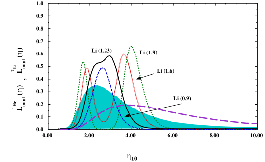
Figure 4.: Likelihood distributions for four values of primordial ⁷Li/H ($10^{10}\times$ ⁷Li = 1.9 (dashed), 1.6 (dotted), 1.23 (solid), and 0.9 (dash-dotted)), and for ⁴He (shaded) for which we adopt $Y_{p}=0.238\pm 0.002\pm 0.005$ (Eq. (1)). Also shown by the long dashed curve is the likelihood function based on the ⁴He abundance from Eq. (2).

5. LiBeB

The production of ⁷Li by galactic cosmic-ray nucleosynthesis shown in Figure 3, is accompanied by the production of the heavier intermediate elements Be and B (Reeves, Fowler, & Hoyle 1970; Meneguzzi, Audouze, & Reeves 1971). Standard GCRN is dominated by interactions originating from accelerated protons and $\alpha$’s on CNO in the ISM, and predicts that BeB should be “secondary” versus the spallation targets, giving $\hbox{$$Be}\propto{\rm O}^{2}$ (Vangioni-Flam, Cassé, Audouze, & Oberto 1990). However, this simple model was challenged by the observations of BeB abundances in Pop II stars, and particularly the BeB trends versus metallicity. Measurements showed that both Be and B vary roughly linearly with Fe, a so-called “primary” scaling. If O and Fe are co-produced (i.e., if O/Fe is constant) then the data clearly contradicts the canonical theory, i.e. BeB production via standard GCR’s.

These observations led to the creation of many new models of cosmic-ray nucleosynthesis (Cassé, M., Lehoucq, R., & Vangioni-Flam, E. 1995; Vangioni-Flam et al. 1996; Ramaty et al. 1997, 1999) which include a dominant primary component of BeB. Such models were discussed here by Cassé, Parizot and Ramaty.

As was discussed here by Deliyannis and Israelian, there is growing evidence that the O/Fe ratio is not constant at low metallicity (Israelian, García-López, & Rebolo 1998; Boesgaard et al. 1999a), but rather increases towards low metallicity. This trend offers another solution to resolve discrepancy between the observed BeB abundances as a function of metallicity and the predicted secondary trend of GCR spallation (Fields & Olive 1998). As noted above, standard GCR nucleosynthesis predicts $\hbox{$$Be}\propto{\rm O}^{2}$, while observations show $\hbox{$$Be}\sim{\rm Fe}$, roughly; these two trends can be consistent if O/Fe is not constant in Pop II. A combination of standard GCR nucleosynthesis, and $\nu$-process production of ¹¹B is consistent with current data.

The determination of abundances from raw stellar spectra requires stellar atmosphere models. The atmospheric models require key input parameters, notably the effective temperature $T_{\rm eff}$ and surface gravity $g$, and assumptions regarding the applicability of local thermodynamic equilibrium (LTE). Unfortunately, there is no standard set of stellar parameters for the halo stars of interest. In practice, different groups derive abundances via different procedures, which give similar results but retain systematic differences. The systematic differences in the data can in fact obscure the BeB-OFe trends one seeks. Thus, to derive meaningful BeB fits, one must systematically and consistently present abundances derived under the same assumptions and parameters for stellar atmospheres.

It is not possible to overly stress the importance of reliable stellar data. The Balmer-line data appear to be self-consistent, and are probably the most reliable. However, because other scales such as those based on the IRFM are commonly used, I would like to point out that there are significant differences in the reported data. To illustrate the point consider for example the case of the star BD $3^{\circ}$ 740. From Axer et al. (1994), whose data is based on the Balmer line method we find this star to have ($T_{\rm eff},\ln g$, [Fe/H]) = (6264, 3.72, -2.36). The beryllium and oxygen abundances for this star was reported by Boesgaard et al. (1999b) and (1999a). When adjusted for these stellar parameters, we find [Be/H] = -13.36, and [O/H] = -1.74. In contrast, the stellar parameters from Alonso et al. (1996a) based on the IRFM (IRFM1) are (6110,3.73,-2.01) with corresponding Be and O abundances of -13.44 and -2.05. Garcia-Lopez et al. 1998 use a calibrated IRFM (IRFM2) based on Alonso et al. (1996b) and take (6295,4.00, -3.00). For these choices, we have [Be/H] = -13.24 and [O/H] = -1.90. Notice the extremely large range in assumed metallicities and the difference in the two so-called IRFM temperatures. While this may not be a typical example of the difference in stellar parameters, it is differences such as this (and this star is not unique) that accounts for the difference in our results and the implications we must draw from them. Uncertainties in [Fe/H] in particular, make modeling extremely difficult. This is especially true of one attempts to model the correlations of BeBO with respect to Fe/H.

Below, we will present results based for the available BeBOFe data based on three methods of analysis. We will refer to these as the Balmer line data and the IRFM1,2 data. Complete results of this analysis can be found in Fields et al. (2000). There are a total of 36 stars with low metallicity OH data. Of these, roughly 2/3 have available data using one of the systematic methods described (Balmer, IRFM1, IRFM2). In each case, one finds a significant slope for [O/Fe] vs [Fe/H] ranging from -0.32 to -0.51.

Of key importance to the modeling of the BeB evolution is the determination of a primary or secondary source for the BeB isotopes. Primary vs secondary is typically ascertained by fitting the BeB data versus a tracer element. Historically, Fe/H was used even though the actual production of LiBeB is independent of [Fe/H]. This is justifiable so long as [O/Fe] is constant. As one can see in the tables below, the data seem to indicate that Be is mostly primary with respect to Fe, and secondary with respect to O/H. (IRFM2 should be considered suspect as the derived parameters were obtained outside the limits of validity of the calibration.) This is what one would expect if [O/Fe] is not constant as the OH data now indicate. B on the other hand shows primary evolution with respect to [O/H] and an even flatter evolution with respect to Fe/H. This too is expected if the $\nu$-process plays a significant role in the production of ¹¹B.

Table 1.: Slopes for Be versus Fe and O.

method	number	tracer	slope	number	tracer	slope
Balmer	22	Fe	$1.39\pm 0.16$	19	O	$1.78\pm 0.19$
IRFM1	22	Fe	$1.23\pm 0.14$	21	O	$1.83\pm 0.19$
IRFM2	18	Fe	$1.18\pm 0.11$	18	O	$1.36\pm 0.09$

Table 2.: Slopes for B versus Fe and O.

method	number	tracer	slope	number	tracer	slope
Balmer	11	Fe	$0.78\pm 0.22$	10	O	$1.23\pm 0.32$
IRFM1	9	Fe	$0.73\pm 0.19$	9	O	$0.98\pm 0.28$
IRFM2	11	Fe	$0.72\pm 0.14$	11	O	$1.02\pm 0.16$

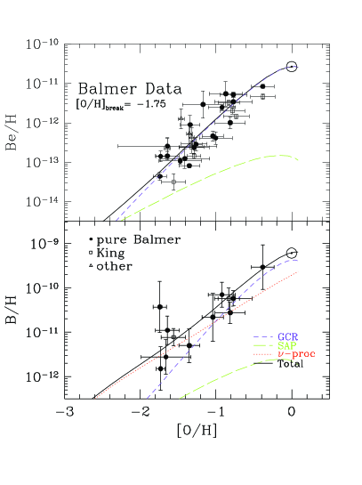
Figure 5.: Be vs O (top panel) and B vs O (bottom panel). Data shown are the Balmer points, which are found to have a break point as indicated. Models are adjusted to have the break point and O/Fe slope of these data.

The models for primary and secondary production of BeB are all physical. What is unclear however, is which is dominant over the history of the Galaxy and at what epoch. If both mechanisms are operative, it is reasonably certain that primary mechanisms should dominate in the early Galaxy and that secondary mechanisms should dominate later. The cross-over or break point can be determined from the data (in principle) by fitting to both linear and quadratic components,

$$\frac{A}{\rm H}=\left(\frac{A}{\rm H}\right)_{\odot}\left[\alpha_{1}\frac{\rm O/H}{({\rm O/H})_{\odot}}+\alpha_{2}\left(\frac{\rm O/H}{({\rm O/H})_{\odot}}\right)^{2}\right]$$ (8)

for $A\in{\rm BeB}$. The resulting coefficients and break points for Be are found in Table 3. As one can see, for Balmer and IRFM1, the break point occurs at low [O/H], indicating that most of the evolution in the observed data has been secondary. To fully resolve this issue, a larger and systematic data set is required.

Table 3.: Break points for Be versus O.

number	method	$\alpha_{1}$	$\alpha_{2}$	[O/H]eq
19	Balmer	$0.042\pm 0.003$	$2.30\pm 0.70$	-1.75
21	IRFM1	$0.034\pm 0.034$	$2.14\pm 0.53$	-1.79
18	IRFM2	$0.111\pm 0.031$	$2.57\pm 0.76$	-1.37

Finally, in Figure 5 (from Fields et al. 2000), the evolution of BeB with respect to O/H is shown in a simple closed box model of chemical evolution. In addition to standard GCR nucleosynthesis, a primary component based on the superbubble accelerated particle spectrum of Bykov (1999) is included along with the neutrino-process for ¹¹B (Fields et al. 2000). The secondary GCR cosmic-ray flux is normalized by the solar abundance of Be and is consisitent with the present cosmic-ray flux scaled by the star formation rate. The break point (from Table 3) determined the relative scaling of the primary component to the secondary one, and the neutrino process is scaled to the solar ¹¹B/¹⁰B ratio.

Acknowledgments.

I would like to thank my collaborators T. Beers, M. Cassé, B. Fields, J. Norris, S. Ryan, E. Skillman, and E. Vangioni-Flam whose work has been summarized here. This work was supported in part by DoE grant DE-FG02-94ER-40823 at the University of Minnesota.

References

Alonso, A., Arribas, S., & Martinez-Roger, C. 1996a, A & AS, 117, 227

Alonso, A., Arribas, S., & Martinez-Roger, C. 1996b, A & A, 313, 873

Axer, M., Fuhrmann, K., & Gehren, T. 1994, A & A, 291, 895

Boesgaard, A.M., King, J.R., Deliyannis, C.P., & Vogt, S.S. 1999a, AJ, 117, 492

Boesgaard, A.M., Deliyannis, C.P., King, J.R., Ryan, S.G., Vogt, S.S., & Beers, T.C. 1999b, AJ, 117, 1549

Bonifacio, P. & Molaro, P. 1997, MNRAS, 285, 847

Bykov, A.M. 1999, in ”LiBeB, cosmic rays and related X-and Gamma- Rays”, eds. Ramaty et al. , ASP, vol. 171, p. 146

Cassé, M., Lehoucq, R., & Vangioni-Flam, E. 1995, Nature, 373, 38

Fields, B. D., Kainulainen, K., Olive, K. A., & Thomas, D. 1996, New Astron., 1, 77

Fields, B.D. & Olive, K.A. 1998, ApJ, 506, 177

Fields, B.D. & Olive, K.A. 1999, ApJ, 516, 797

Fields, B.D. & Olive, K.A. 1999, New Astron., 4, 255

Fields, B.D., Olive, K.A., Vangioni-Flam, E. & Cassé, M. 2000, astro-ph/9911320.

García-López, R.J., et al. , Ap.J. 500 (1998)

Israelian, G., García-López, R.J., & Rebolo, R. 1998, ApJ, 507, 805

Izotov, Y.I. & Thuan, T.X. 1998, ApJ, 500, 188.

Izotov, Y.I., Thuan, T.X., & Lipovetsky, V.A. 1994 ApJ 435, 647

Izotov, Y.I., Thuan, T.X., & Lipovetsky, V.A. 1997, ApJS, 108, 1

Meneguzzi, M. , Audouze, J., & Reeves, H. 1971, A&A, 15, 337

Olive, K.A., Steigman, G. & Skillman, E.D. 1997, ApJ, 483, 788

Olive, K.A. & Skillman, E. 2000, in preparation.

Pagel, B.E.J., Simonson, E.A., Terlevich, R.J. & Edmunds, M. 1992, MNRAS, 255, 325

Ramaty, R., Kozlovsky, B., Lingenfelter, R.E., & Reeves, H. 1997, ApJ, 488, 730

Ramaty, R., Scully, S., Lingenfelter, R. and Kozlovsky, B. 1999 (astro-ph/9909021)

Reeves, H., Fowler, W.A., & Hoyle, F. 1970, Nature, 226, 727

Ryan, S.G., Beers, T.C., Olive, K.A., Fields, B.D., & Norris, J.E. 2000, ApJL, in press (astro-ph/9905211)

Ryan, S.G., Norris, J.E., & Beers, T.C. 1999, ApJ, 523, 654

Skillman, E., & Kennicutt 1993, ApJ, 411, 655

Skillman, E., Terlevich, R.J., Kennicutt, R.C., Garnett, D.R., & Terlevich, E. 1994, ApJ, 431, 172

Spite, F. & Spite, M. 1982, A&A, 115, 357

Vangioni-Flam, E., Cassé, M., Audouze, J., & Oberto, Y. 1990, ApJ, 364, 568

Vangioni-Flam, E., Cassé, M., Fields, B.D., & Olive, K.A. 1996, ApJ, 468, 199