A time-delay determination from VLA light curves of the CLASS gravitational lens B1600+434

Abstract

We present Very Large Array (VLA) 8.5-GHz light curves of the two lens images of the Cosmic Lens All Sky Survey (CLASS) gravitational lens B1600+434. We find a nearly linear decrease of 18–19% in the flux densities of both lens images over a period of eight months (February-October) in 1998. Additionally, the brightest image A shows modulations up to $11\%$ peak-to-peak on scales of days to weeks over a large part of the observing period. Image B varies significantly less on this time scale. We conclude that most of the short-term variability in image A is not intrinsic source variability, but is most likely caused by microlensing in the lens galaxy. The alternative, scintillation by the ionized Galactic ISM, is shown to be implausible based on its strong opposite frequency dependent behavior compared with results from multi-frequency WSRT monitoring observations (Koopmans & de Bruyn 1999).

From these VLA light curves we determine a median time delay between the lens images of $47^{+5}_{-6}$ d (68%) or $47^{+12}_{-9}$ d (95%). We use two different methods to derive the time delay; both give the same result within the errors. We estimate an additional systematic error between $-$8 and +7 d. If the mass distribution of lens galaxy can be described by an isothermal model (Koopmans, de Bruyn & Jackson 1998), this time delay would give a value for the Hubble parameter, H₀=$57^{+14}_{-11}$ (95% statistical) ${}^{+26}_{-15}$ (systematic) km s^-1 Mpc^-1 ($\Omega_{\rm m}$=1 and $\Omega_{\Lambda}$=0). Similarly, the Modified-Hubble-Profile mass model would give H₀=$74^{+18}_{-15}$ (95% statistical) ${}^{+22}_{-22}$ (systematic) km s^-1 Mpc^-1. For $\Omega_{\rm m}$=0.3 and $\Omega_{\Lambda}$=0.7, these values increase by 5.4%. We emphasize that the slope of the radial mass profile of the lens-galaxy dark-matter halo in B1600+434 is extremely ill-constrained. Hence, an accurate determination of H₀ from this system is very difficult, if no additional constraints on the mass model are obtained. These values of H₀ should therefore be regarded as indicative.

Once H₀ (from independent methods) and the time delay have been determined with sufficient accuracy, it will prove more worthwhile to constrain the radial mass profile of the dark-matter halo around the edge-on spiral lens galaxy at $z$=0.4.

1 Introduction

Gravitational lens systems can be used to determine the Hubble parameter, H₀ (Refsdal 1964). However, both a good mass model of the lens galaxy as well as a time delay between an image pair are necessary ingredients to accomplish this. The mass model can be constrained from the lens-image properties, whereas a time delay can be obtained through correlations between two image light curves. Intrinsic source variability should occur in all light curves, lagging by time delays which depend on the source and lens redshifts, the lens-mass distribution and the cosmological parameters, most prominently H₀ (e.g. Schneider et al. 1992).

Recently, time delays and values of H₀ were determined from several different gravitational lens (GL) systems: Q0957+561 (e.g. Schild & Thomson 1997; Kundić et al. 1997a; Haarsma et al. 1997, 1999; Press, Rybicki & Hewitt 1992; Pelt et al. 1994; Pelt et al. 1996; Grogin & Narayan 1996; Bernstein et al. 1997; Fischer et al. 1997; Falco et al. 1997; Bernstein & Fischer 1999; Barkana et al. 1999), PG1115+080 (e.g. Schechter et al. 1997; Courbin et al. 1997; Kundić et al. 1997b; Keeton & Kochanek 1997; Barkana 1997; Saha & Williams 1997; Pelt et al. 1998; Impey et al. 1998; Romanowsky & Kochanek 1999), B0218+357 (e.g. Biggs et al. 1999), B1608+656 (e.g. Fassnacht et al. 1999; Koopmans & Fassnacht 1999) and PKS 1830-211 (e.g. van Ommen et al. 1995; Lovell et al. 1998; Kochanek & Narayan 1992; Nair, Narasimha & Rao 1993).

Assuming that the lens galaxies in these GL systems can be described by an isothermal mass distribution, one finds that the values of H₀ derived from these GL systems – except for PG1115+080 – are consistent within their 1-$\sigma$ errors and agree with the local, SNe Ia and S-Z determinations of H₀ (e.g. Koopmans & Fassnacht 1999). However, one has to keep in mind that a similar mass-sheet or change in the radial mass profile of the lens galaxies introduce a similar change in the determination of H₀ from each of these GL systems (e.g. Falco, Gorenstein & Shapiro 1985; Gorenstein, Shapiro & Falco 1988; Grogin & Narayan 1992; Keeton & Kochanek 1997; Wucknitz & Refsdal 1999). Hence, also for mass models other than isothermal one might expect the values of H₀ to agree to first order. Strong deviations of the lens-galaxy mass distribution from isothermal, however, would lead to systematic differences between the values of H₀ determined from lensing and those determined from other methods.

In this paper, we present a determination of the time delay between the two lens images of the CLASS gravitational lens B1600+434, using the light curves obtained during an eight-month VLA 8.5-GHz monitoring campaign. In section 2, we describe the VLA observations of B1600+434 and the data reduction. In section 3, we apply the minimum dispersion method from Pelt et al. (1996) and the PRH-method (Press et al. 1992) to determine a time delay between the lens images and use that to estimate a tentative value for H₀, keeping the above-mentioned problems with the mass-model degeneracies in mind. In section 4, our conclusions are summarized.

2 Data & Reduction

2.1 Observations

We observed the CLASS gravitational lens B1600+434 (Jackson et al. 1995; Jaunsen & Hjorth 1997; Koopmans, de Bruyn & Jackson 1998) with the VLA in A- and B-arrays at 8.5 GHz (X-band), during the period 1998 February 13 to October 14. The typical angular resolution of the radio images ranges from about 0.2 arcsec in A-array to 0.7 arcsec in B-array, sufficient to resolve the 1.4-arcsec double. In total we obtained 75 epochs of about 30 min each, including phase- and flux-calibrator observations and slewing time. The average time interval between epochs was 3.3 days. A typical observing run consisted of the sequence listed in Table 1. This sequence was repeated, typically twice, until about 30 min observing time was filled. Several epochs consisted of only 10 or 20 min, making it necessary to reduce the number of sequences, or the time spent on each of the sources. At the end of a sequence, we again observed 2 min on the phase calibrator J1549+506 (Fig.1; Patnaik et al. 1992).

The flux calibrator, B1634+627 (3C343), is a slightly extended steep-spectrum source (Fig.1; e.g. van Breugel et al. 1992), which should not be variable. Its flux density at 8.5 GHz is 0.84$\pm$0.01 Jy, which we obtained with the Westerbork-Synthesis-Radio-Telescope (WSRT) in December 1998. This value agrees with the average flux density of 0.83 Jy, obtained with the 26-m University of Michigan Radio Astronomy Observatory (UMRAO) telescope, which has been monitoring this source for the past 15 years. We use the WSRT flux-density determination to bring all flux densities to the correct absolute scale (Sect.2.4).

Table 1: Basic observing sequence on B1600+434 and the phase and flux calibrators. This sequence was repeated typically twice per session.

1	J1549+506	2 min	phase calibrator
2	B1634+627	2 min	flux calibrator
3	B1600+434	6 min	CLASS gravitational lens
4	B1634+627	2 min	flux calibrator

2.2 Calibration

The initial flux and phase calibration is done in the NRAO data-reduction package AIPS (version 15OCT98). We fixed the flux density of the phase calibrator at 1.17 Jy at all epochs and subsequently solve for the telescope phase and gain solutions. The phase calibrator (J1549+506; Patnaik et al. 1992) is an unresolved flat-spectrum point source ($<$10 mas) at 8.5 GHz when observed with the VLA in A-array (Fig.1). A single delta function is therefore sufficient to describe the source structure. Because the phase calibrator is a flat spectrum and compact source, it could vary significantly over a monitoring period of eight months. Thus, the flux density of 1.17 Jy could be wrong by a large factor. We therefore use the flux calibrator to determine the proper flux-density scale and correct for ‘variability’ introduced in both images of B1600+434, due to intrinsic flux-density variability of the phase-calibrator. As we will see in Sect.2.4, this strategy works well.

We smooth (1-min intervals) and interpolate the phase and gain solutions between the phase calibrator scans for the entire observation period of about 30 min. These are then used to determine initial phase and gain solutions for the flux calibrator B1634+627 and the gravitational lens system B1600+434. No flagging was done in AIPS, because it is hard to assess if phase and/or gain errors can be corrected through self-calibration. Flagging is only done in the DIFMAP package (Shepherd 1997), where the visibility amplitudes and phases can be compared with a model of the source structure and possibly be corrected through self-calibration. Only if the latter fails, do we manually flag those visibilities which most strongly deviate from the model.

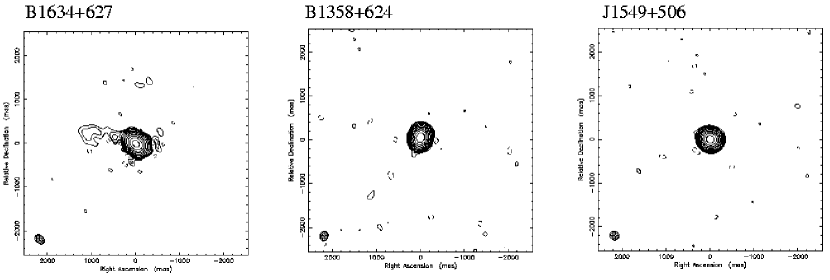
Figure 1: VLA 8.5-GHz A-array images of the flux density calibrators B1634+627 and B1358+624, and the phase calibrator J1549+506 (epoch 1998 May 25). Contours starts at 3-$\sigma$ and increase by factors of two. The lowest contours are 0.53, 0.56 and 0.56 mJy beam^-1 for B1634+627, B1358+624 and J1549+506, respectively.

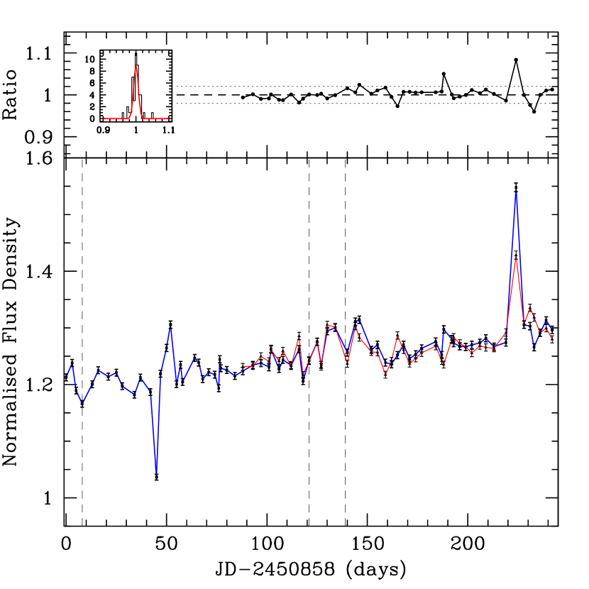
Figure 2: The lower panel shows the light curves of B1634+627 (squares) and B1358+624 (triangles), normalized by the flux density of J1549+506 (i.e. 1.17 Jy; see Sect.2.1). The upper panel shows the ratio of the two curves, where they overlap. The small sub panel shows a histogram of this ratio, fitted by a Gaussian with a 1-$\sigma$ value of $\approx$0.7%. The dotted lines in the upper panel indicate the $\pm$3-$\sigma$ region from the Gaussian fit. The error bars on the light curves are 0.7%$/\sqrt{2}\approx 0.5\%$ (Sect.2.7), assuming the errors on both light curves are similar. The vertical dashed lines indicate the array changes D$\rightarrow$A, A$\rightarrow$BnA and BnA$\rightarrow$B, respectively, from left to right.

2.3 Imaging and model fitting

First we make maps of B1600+434 for all epochs in DIFMAP (version 2.2c), using a process of iterative model fitting and self-calibration. Because the two lens images are compact ($\leq$1 mas) at 8.5-GHz, determined from VLBA observations (Fig.3), and also show no extended emission from either the lens or quasar on mas to arcsec scales in MERLIN 5-GHZ observations (Koopmans et al. 1998), we can safely model the lens image structure by two delta functions, for which we determine the positions and flux densities. We fit these delta functions to the visibilities, until the model-$\chi^{2}$ converges. We perform a phase-only self-calibration, using this model. Typically, this decreases the $\chi^{2}$ of the model and the rms noise in the map significantly. We repeat this process several times, until no further decrease in either $\chi^{2}$ or rms noise level is obtained. Finally, a global gain-self-calibration is performed, solving for small gain errors of each telescope. This gain-self-calibration does not significantly change the flux densities of the images (i.e. changes that are much less than the statistical error on the flux densities) and individual telescope gain corrections are typically less than a few percent. We repeat the process of model fitting and self-calibration, until it converges again. The visibilities are then compared with the best model and obviously errant points are manually flagged. Once more, we iterate between model fitting and self-calibration until convergence is reached. Finally, we average the visibilities over 300 sec and repeat the convergence process, after having flagged those points which still deviate significantly ($\ga$3-sigma) from the model.

The flux-density ratio between images A and B changes by at most a few tenths of a per cent before and after these calibration cycles, as long as there are no visibilities which deviate by orders of magnitude from the model. The reduced-$\chi^{2}$-value of the final model fit typically lies between 1.0 and 1.1. The residual maps show no spurious features due to bad visibilities. Fig.3 shows a radio map of B1600+434, created from the combined A-array data-sets of seven epochs.

2.4 Flux calibration

We subsequently make maps of the flux calibrator, B1634+ 627, using the same procedure as for B1600+434. B1634+627 can be well represented by a single Gaussian component with a 1-$\sigma$ major axis of 90 mas, an axial ratio of 0.8 and a position angle of 70 deg, in broad agreement with the source structure as seen in 50-cm VLBI images (Nan et al. 1991). We use this component to model fit the image structure and self-calibrate the visibilities. We subsequently remove this Gaussian component and clean the map to find a better description of the extended structure of the source. The ratio between the flux density in the Gaussian component and the total flux density in all extended emission (seen with the VLA in A and B-arrays on a scale $\la$10 arcsec) is 0.98. The ratio is independent of epoch (within the errors). The determination of the flux density using a single Gaussian component is better defined than the flux density derived from an iterative cleaning procedure. The latter procedure seems to introduce $\la$1% errors, depending on how the maps were cleaned, what array was used and inside which box the total flux density was determined. Using only a single Gaussian to represent the source, does not involve cleaning or choosing a box size.

We determine the normalized light curve of the flux calibrator B1634+627 by dividing its flux-density light curve by the flux density of 0.84$\pm$0.01 Jy (Sect.2.1). The resulting curve shows a linear increase of approximately 5% over the eight-month observing period, which we attribute to a similar change in the flux density of the flat-spectrum phase calibrator, J1549+506. We also see that we have overestimated the flux density of B1634+627 by some 20–30%. In other words, our initial estimate of the flux density of the phase calibrator, based on the value given in the VLA calibrator manual, was 20–30% too high, which comes as no surprise for a variable flat-spectrum radio source.

From May 12 1998 onwards, we added a second flux calibrator, B1358+624 (Fig.1), to the observations, to estimate the reliability of the flux-density determination of B1634+627. We followed the same calibration and mapping procedure as for B1634+627. B1358+624 also shows the same 5% linear increase in flux density, supporting the idea that this is the result of variability of the phase calibrator. We scale the flux density curve of B1358+624 to fit the calibrated light curve of B1634+627 and find its flux density to be 1.14$\pm$0.02 Jy. The final normalized flux density curve of B1358+624 is also shown in Fig.2.

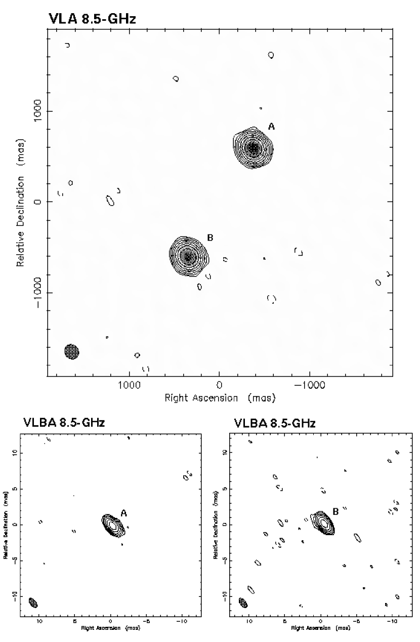
Figure 3: Top: VLA 8.5-GHz A-array image of B1600+434, showing the two compact lens images A and B. The image was created from a combined data set from 7 different epochs. The contours indicate (-3,3,6,12,24,48,96,192,384)$\times$rms noise, where the rms noise is 0.059 mJy beam^-1. Bottom: VLBA 8.5-GHz images of the lens components B1600+434 A and B (5-h integration) taken 1996 November 4. For a full discussion on the VLBA data reduction see Koopmans et al. (1999), where this has been explained in detail for B1127+385, which was observed during the same run as B1600+434. The contours indicate (-2,2,4,8,16,32,64) per cent of the map peak, where the map peak is 30.1 (23.4) mJy beam^-1 for image A (B). Both lens images show no sign of any extended structure larger than about 1 mas.

2.5 Light curves of B1600+434

To correct the light curves of B1600+434 for flux-density calibration errors, we divide them by the average of the normalized light curves of B1634+627 and B1358+624.

We assume that both flux calibrators do not vary intrinsically over the eight-month observing period. We also assume that the phase and gain solutions found from J1549+ 506 do not change significantly over a time span of several minutes, such that interpolation can be used to make a first-order correction for phase and gain errors in data of B1600+434, B1634+627 and B1358+624. This flux density correction removes the largest errors in the light curves of B1600+434, after which only statistical errors, second-order systematic errors and intrinsic variations are left. Any deviations between the two normalized light curves are most likely due to short-term calibration errors, either instrumental or atmospheric. The final flux-calibrated light curves of the lens images A and B are shown in Fig.4. The calibrated flux-densities are listed in Table 2.

Both light curves show a gradual decrease of about 0.02 mJy day^-1 over a period of 243 days (Sect.3.1). Superposed on this gradual long-term variability, image A also exhibits strong (up to 11% peak-to-peak) modulations on a time scale of a few days to several weeks. Image B only shows a few (up to 6% peak-to-peak) features, but separated in time by about one month or more. The modulation indices (i.e. fractional rms variability) around the gradual long-term decrease in flux density (indicated by the dashed lines in Fig.4) are 2.8% and 1.9% for images A and B, respectively.

Table 2: The calibrated flux-densities of B1600+434-A and B at 8.5-GHz, during the VLA A and B-arrays monitoring campaign in 1998. The 1-$\sigma$ errors on the flux densities are 0.8% for days 0–84 and 0.7% for days 88–243. The six ‘outliers’ (Sect.2.7) are indicated by a star (*) and their estimated error ($\sigma_{\rm S}$) is given in the comments.

Epoch	Date	Start	Array	$S_{8.5}^{\rm A}$	$S_{8.5}^{\rm B}$	Comments
JD$-$2450858		(LST)		(mJy)	(mJy)
0	13/2/98	12:37:50	D$\rightarrow$A	26.294	23.777
3	16/2/98	12:26:00	D$\rightarrow$A	26.450	24.055
5	18/2/98	12:46:27	D$\rightarrow$A	27.164	24.243	Light snow
8	21/2/98	12:05:30	A	28.004	24.177
13	26/2/98	13:46:04	A	27.104	23.210	Wind $\geq$ 5 m/s
16	1/3/98	10:34:48	A	26.776	23.271
21	6/3/98	12:14:57	A	26.408	23.303
25	10/3/98	11:59:00	A	27.061	23.153
28	13/3/98	09:16:49	A	26.491	23.235
34	19/3/98	07:54:15	A	26.744	23.065
37	22/3/98	09:42:07	A	26.783	22.799
42	27/3/98	13:21:50	A	26.803	23.066	Wind $\geq$ 5 m/s
45	30/3/98	05:41:09	A	27.136	22.606	Overcast+Light snow
47	1/4/98	10:02:44	A	27.002	22.261
50	4/4/98	15:49:50	A	26.025	21.456	Wind $\geq$ 5 m/s
52	6/4/98	10:12:52	A	25.577	22.023
55	9/4/98	08:31:26	A	27.441	22.396
57	11/4/98	06:54:08	A	25.514	22.479
58	12/4/98	06:19:50	A	25.962	22.062	Wind $\geq$ 5 m/s
64	18/4/98	07:26:30	A	26.111	22.842
66	20/4/98	07:48:11	A	26.638	22.600
68	22/4/98	02:41:30	A	25.732	22.508
71	25/4/98	05:58:44	A	25.336	22.691
74	28/4/98	06:17:20	A	25.950	22.730
76	30/4/98	05:39:05	A	26.836	22.846
77	1/5/98	00:05:54	A	27.057	22.481
77	1/5/98	09:04:22	A	26.304	22.637
80	4/5/98	07:52:35	A	25.902	22.224
84	8/5/98	05:07:09	A	26.134	22.354
88	12/5/98	06:51:32	A	26.299	21.904
93	17/5/98	10:01:50	A	25.702	21.712	Wind $\geq$ 5 m/s
97	21/5/98	03:10:00	A	26.851	21.833
101	25/5/98	04:00:04	A	25.893	21.751
102	26/5/98	09:26:00	A	24.151	21.711
106	30/5/98	03:41:38	A	24.937	21.770
108	1/6/98	04:02:51	A	25.929	21.589
112	5/6/98	05:17:17	A	24.140	21.699

Table 2: (Continued).

Epoch	Date	Start	Array	$S_{8.5}^{\rm A}$	$S_{8.5}^{\rm B}$	Comments
JD$-$2450858		(LST)		(mJy)	(mJy)
116	9/6/98	04:01:50	A	23.423	20.862
118	11/6/98	03:23:33	A	24.701	21.342
121	14/6/98	06:11:18	BnA	25.760	22.131	Wind $\geq$ 5 m/s
125	18/6/98	02:56:18	BnA	24.715	21.547
127	20/6/98	03:18:14	BnA	23.345	20.991	Power outage
130	23/6/98	02:36:46	BnA	23.458	21.081	Wind $\geq$ 5 m/s
134	27/6/98	05:20:40	BnA	23.052	21.005
140	3/7/98	03:57:00	B	23.918	21.100	Thunder+showers
144	7/7/98	22:47:35	B	24.707	21.187	Thunderstorms in area
146∗	9/7/98	02:58:38	B	23.389	20.907	Showers; Erratic behavior Tsys; ($\sigma_{\rm S}$=1.8%)
152	15/7/98	05:39:21	B	24.137	20.719
155	18/7/98	05:28:50	B	24.099	21.089
159	22/7/98	05:12:50	B	24.286	20.821	Distant sheet lightening
162	25/7/98	05:00:56	B	24.500	20.700	Showers
165∗	28/7/98	04:46:32	B	24.128	20.462	Wind $\geq$ 5 m/s; Showers;
						$\approx$50% gradual decrease in Tsys; ($\sigma_{\rm S}$=1.9%)
168	31/7/98	03:00:30	B	24.057	20.286
171	3/8/98	04:24:45	B	24.957	20.137
174	6/8/98	03:13:03	B	24.480	19.980
177	9/8/98	04:01:12	B	24.709	20.065
183	15/8/98	03:37:24	B	24.159	19.894
187	19/8/98	03:21:38	B	23.741	20.186
188∗	20/8/98	22:40:51	B	24.239	21.143	Wind $\geq$ 5 m/s; Showers;
						Erratic behavior Tsys; ($\sigma_{\rm S}$=3.4%)
192	24/8/98	01:02:27	B	24.485	19.878
193	25/8/98	22:49:40	B	23.073	19.895	Wind $\geq$ 5 m/s
196	28/8/98	02:22:42	B	22.522	19.650	Thunderstorms in area
199	31/8/98	02:34:40	B	23.604	19.722
202	3/9/98	03:22:50	B	23.952	19.916
206	7/9/98	02:07:01	B	23.218	19.752
209	10/9/98	03:24:54	B	24.017	20.142	Wind $\geq$ 5 m/s
213	14/9/98	01:39:17	B	23.235	20.330
219	20/9/98	01:16:10	B	23.369	20.015
223∗	24/9/98	21:57:00	B	22.766	20.952	Rapid $\approx$20% fluctuations in Tsys; ($\sigma_{\rm S}$=4.8%)
227	28/9/98	20:11:22	B	22.190	19.582
230∗	1/10/98	22:59:00	B	22.132	19.307	Wind $\geq$ 5 m/s; Erratic behavior Tsys; ($\sigma_{\rm S}$=2.0%)
232∗	3/10/98	22:51:04	B	22.547	18.848	Wind $\geq$ 5 m/s; Erratic behavior Tsys; ($\sigma_{\rm S}$=3.2%)
235	6/10/98	22:09:00	B	21.717	18.513
240	11/10/98	01:52:41	B	22.826	19.112	Wind $\geq$ 5 m/s
243	14/10/98	01:10:54	B	22.789	19.080	Wind $\geq$ 5 m/s

2.6 External variability

In Koopmans & de Bruyn (1999) it is shown that most of the observed short–term variability is of external origin (at the 14.6-$\sigma$ confidence level). A number of possible causes of this short-term variability are examined: (i) scintillation caused by the ionized component of the Galactic ISM and (ii) radio microlensing of a core-jet structure by massive compact objects in the lens galaxy. Based on Galactic scintillation models (e.g. Narayan 1992; Taylor & Cordes 1993; Rickett et al. 1995), one predicts a strong increase in the modulation index towards longer wavelengths in the case of scintillation, whereas a strong decrease is observed in the long-term monitoring data obtained with the Westerbork-Synthesis-Radio-Telescope (WSRT) at 1.4 and 5 GHz (Koopmans & de Bruyn 1999). The quantitative decrease in the modulation index from 5 to 1.4 GHz, seen in this WSRT monitoring data, agrees remarkably well with that predicted from microlensing simulations, but differs by a factor of $\approx$8 from that predicted from the scintillation models. A strong case for the occurrence of radio microlensing in B1600+434 can therefore be made, which can complicate a straightforward determination of the time delay from these light curves. However, based on two independent methods of analysis (Sect.3.1), we are convinced that the obtained time delay is little affected by this external variability.

2.7 Error analysis

The errors on the light curves are a combination of thermal noise errors and systematic errors (e.g. modeling, self-calibration, instrumental, atmospheric, etc.). The noise errors on the $\ga$1 Jy flux density calibrators are of the order of 0.01% after a few minutes of integration. The noise error on each of the lens images is about 0.3%, determined from the residual maps (i.e. the radio image after subtracting the model of the source structure). This noise level agrees well with the theoretically expected value for the typical integration time of $\approx$10 min.

To estimate the systematic errors (i.e. systematic in the sense that they affect the flux-densities of both image A and B), we compare the two normalized light curves of B1634+627 and B1358+624. In Fig.2, we see that both curves follow each other extremely well. Their ratio has an rms scatter of 0.7%, determined from fitting a Gaussian to its distribution function. Assuming the errors on both normalized light curves are similar, the errors on the individual points are therefore 0.7$/\sqrt{2}$$\approx$0.5%. This error is probably a mixture of modeling, self-calibration and short-term atmospheric and instrumental effects, which are hard to remove. We conservatively assume that the data of B1600+434 contains a similar 0.5% error.

During the B-array observations, six points lie clearly outside the 3-$\sigma$ region (Fig.2, upper panel), whereas during the A- and BnA-array observations, the ratio seems much more more stable. This stability during A- and BnA-array observations is reflected in the extremely small scatter in the measured distance between the two lens images (Fig.4, upper panel), which is similar to the theoretical expectation value of $\Delta r_{\rm AB}$=0.5 mas, where we used $\Delta r_{\rm AB}=\sqrt{2}\times\Delta\theta/(2\cdot{\rm SNR})$, with $\Delta\theta$ being the beam size of 0.2 (0.7) arcsec in A-array (B-array) and SNR the signal-to-noise ratio of about 1/0.003$\approx$330.

The six ‘outliers’ are given an error equal to their difference in normalized flux density divided by $\sqrt{2}$, which is the expectation value if their errors are equal and drawn from a Gaussian distribution. The errors are 1.8–4.8%. Although this approach appears rather ad-hoc, we will later on in the determination of a time-delay use the light-curves both with and without these points, to investigate the effect they have on our analysis. As it will turn out, the effect is negligible (Sect.3.1.3).

To explain why we find these outliers, we investigated the system temperature (T_sys) as function of time. Fast or systematic changes in T_sys could indicate instrumental, atmospheric (e.g. precipitation) problems or electromagnetic interference. During day 223 (i.e. JD$-$2450858), T_sys shows rapid changes of up to 20% on time scales of a few minutes, which could explain the large difference in the normalized flux density from the running mean and the large difference in the ratio between the normalized flux densities of B1634+627 and B1358+624 from unity. During the observations, cumuloform type clouds were forming with $\sim$50% sky coverage over the array, possibly indicating strong interference caused by nearby thunderstorms (i.e. lightning). Also the other five outliers, during B-array, show some erratic behavior of T_sys, although less serious than on day 223 and typically for only several of the telescopes. Only day 165 shows a $\approx$50% decrease in T_sys over a 1h time interval for all telescopes. Because this decrease is relatively smooth, gain-self-calibration can solve for most of the errors. No such behavior is found between days 45 to 52 (in A-array) for example, which shows a much more gradual change in T_sys and maximum differences less than 10%. On day 45, T_sys behaves similar to epochs with no severe data problems. Its system temperature, however, is on average higher, which explains why the normalized flux density is lower. The higher system temperature for each of the telescopes is explained by the fact that it was snowing during the observations over the entire array (100% sky coverage). However, because T_sys changes only gradually, the error on the corrected flux densities of images A and B will be similar to those of the other well behaved epochs.

Finally, we average the overlapping parts of the two normalized light curves, such that the errors decrease by a factor $\sqrt{2}$. Adding all errors quadratically, we find a total error of 0.8% on the light curves of B1600+434 A and B in the region where the normalized flux calibrator light curves do not overlap, and 0.7% where they do overlap. In Sect.3.1.4, we show that an error of 0.7–0.8% is statistically highly plausible, lending credibility to it.

Moreover, at a given epoch the systematic errors in the flux densities of images A and B are the same (i.e. because of their small angular separation of 1.4 arcsec, instrumental and atmospheric errors should be the same, as well as initial phase calibrator errors, which have been transferred to both images). Their flux density ratio is therefore much better determined and has an error of only $\sqrt{2}\times$0.3% $\approx$0.4%. The errors at different epochs, however, are independent, which is important if the light curves are shifted to determine a time delay (Sect.3.1).

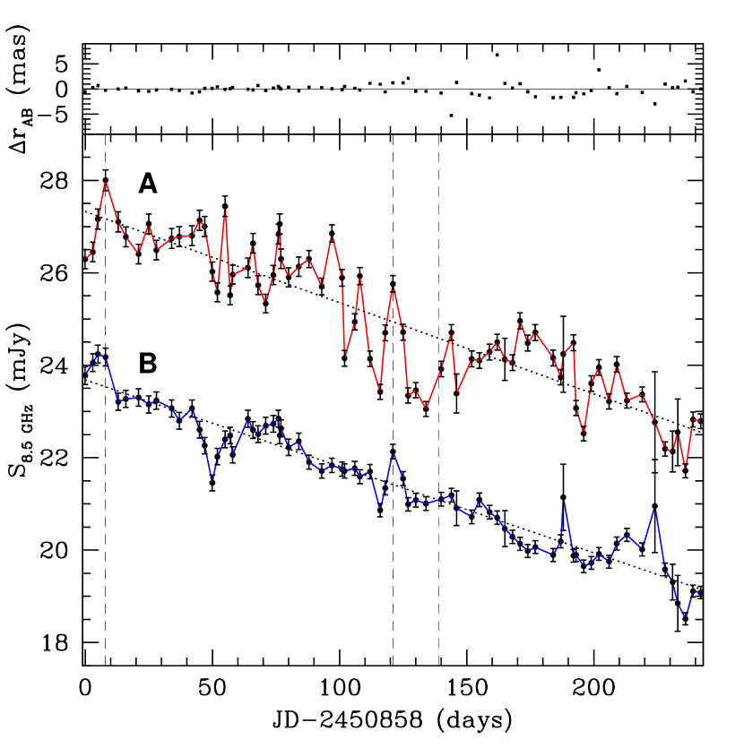
Figure 4: Lower panel: VLA 8.5-GHz light curves of B1600+434 A and B, starting Febr. 13 1998. The error bars indicate the 1-$\sigma$ error, including systematic errors. The dotted lines are linear fits to the light curves. The vertical dashed lines indicate the array changes D$\rightarrow$A, A$\rightarrow$BnA and BnA$\rightarrow$B, respectively, from left to right. Upper panel: The distance between images A and B, minus its median distance of 1392 mas (mean distance is also 1392 mas).

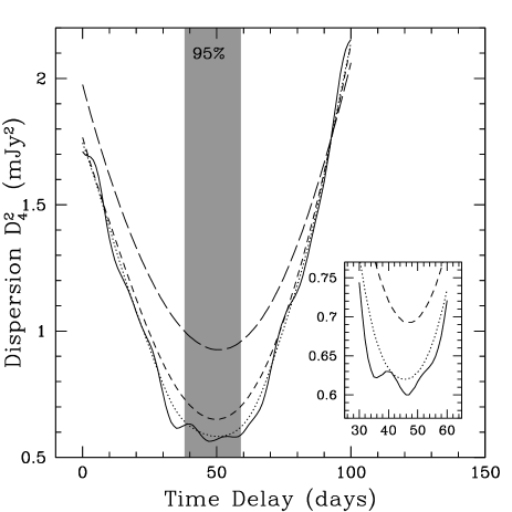
Figure 5: Left: Dispersion measure $D^{2}_{4}$ (Pelt et al. 1996) between the light curves of images A and B, using $r_{\rm AB}=1.212$. The decorrelation time scale $\delta$=1, 2, 4 and 8 (lower to upper curve), in units of the average time span between observations (i.e. 3.3 days). The dispersion minimizes between days 46–51. The shaded region indicates the 95% statistical confidence region for the minimum-dispersion time delay. Right: Time-delay PDFs from Monte-Carlo simulations (Sect.3.1.2). Shown are the four distributions for $\delta$=1, 2, 4 and 8. The bin size is 1 day and the dashed lines indicate the region containing 95% of the time-delay PDF.

3 Analysis

In this section we use the VLA 8.5-GHz light curves to put constraints on the time delay between the two lens images.

3.1 The time delay

A simple estimate of the time delay could be obtained, using the long-term gradients in both light-curves combined with the intrinsic flux-density ratio. Fitting a straight line to both curves (Fig.4) gives a flux-density decrease of $-$1.98$\cdot 10^{-2}$ mJy day^-1 for curve A and $-$1.87$\cdot 10^{-2}$ mJy day^-1 for curve B. Correcting the latter value by multiplying it by the flux-density ratio of 1.212 (see below) gives $-$2.27$\cdot 10^{-2}$ mJy day^-1. This value is different from that of curve A by some 15%, indicating that the rate of decrease in the flux-density changes over the time-scale of the observations. One can therefore not simply divide the difference in flux-density between curve A and curve B (multiplied by the intrinsic flux-density ratio) by the rate of decrease in flux-density to obtain a time delay.

Moreover, the rapid strong modulations seen in the light curve of image A (Fig.4) makes interpolation questionable. This excludes the use of either the $\chi^{2}$-minimization or cross-correlation methods in determining the time delay, because the light curves have to be resampled on a similar grid through some form of interpolation.

We have therefore chosen to use the non-parametric minimum-dispersion method developed by Pelt et al. (1996). In Sect.3.1.4 we will also derive the time delay using the PRH-method from Press, Rybicki & Hewitt (1992). As an additional constraint we use a flux density ratio of 1.212$\pm$0.005, determined from 28 epochs of VLA 8.5-GHz observations during a period of $\approx$4 months in 1996-1997 in which there was relatively little variability (C.B. Moore 1999, private communication). Because this period is significantly longer than the time delay between images A and B (Sect.3.1.2), the low rms variability implies that the above value should represent the intrinsic flux density ratio quite closely. However, we emphasize the preliminary nature of this value, which might still change slightly in a final analysis.

Because the fainter image (B) lags the brighter image (A) (Koopmans et al. 1998) and the flux densities of both images decrease almost linearly over a period of eight months, the flux-density ratio will on average be smaller than the flux-density ratio of 1.212. Shifting the light curve of image B back in time will increase the flux-density ratio between the overlapping parts of the light curves. When the shift in time equals the time delay between the lens images, the average flux-density ratio between the light curves should be 1.212. Hence, if we multiply the light curve of image B with the flux-density ratio of 1.212, we expect the minimum dispersion between the two light curves to occur near the intrinsic time delay.

3.1.1 Minimum dispersion method

From the simple consideration that the observed flux-density ratio ($\approx$1.16) is smaller than the ratio of 1.212, we immediately see that image B lags image A in time, in agreement with lens models (Koopmans et al. 1998). Thus, the time delay $\Delta t_{\rm B-A}$ is positive. A composite light curve is created by multiplying light curve B with the flux-density ratio of 1.212 and shifting it backward in time by $\Delta t_{\rm B-A}$. The dispersion of the composite light curve is calculated as in Pelt et al. (1996), using the dispersion measure

$$D^{2}_{4}(\Delta t)=\frac{\sum_{n=1}^{N-1}\sum_{m=n+1}^{N}S_{\rm m,n}W_{m,n}G_{m,n}(C_{\rm n}-C_{\rm m})^{2}}{\sum_{m=n+1}^{N}S_{\rm m,n}W_{m,n}G_{m,n}}$$

where $C_{\rm n}$ is the $n$-th point on the composite light curve and $G_{m,n}$=1 (0), if $C_{\rm n}$ and $C_{\rm m}$ are from different (the same) light curves. We calculate the dispersion for all time delays $\Delta t_{\rm B-A}$=0–100 days, in steps of 1 day. This process is performed for four different decorrelation time scale, $\delta$=1,2,4,8, in units of the average time span between epochs, i.e. 3.3 days. We use a decorrelation weight function $S_{\rm m,n}=\exp[-(t_{\rm m}-t_{\rm n})^{2}/(2\Delta^{2})]$, where $\Delta=3.3\times\delta$ is the decorrelation time scale in days. The statistical weights are $W_{m,n}=(W_{n}W_{m})/(W_{n}+W_{m})$, where $W_{i}=1/\sigma_{i}^{2}$ and $\sigma_{i}$ the 1-$\sigma$ error on the flux density at the $i$-th epoch.

In Fig.5 the dispersion $D^{2}_{4}$ is plotted versus the time delay, for $\delta$=1,2,4 and 8. The dispersion minimizes near a time delay of 46 to 51 days.

3.1.2 Median time delay and statistical error range

To determine a statistical confidence region for the time delay, we performed Monte-Carlo simulations for $\delta$=1,2,4 and 8. First, we re-sampled the light curves, using the sampling-interval distribution determined from the VLA observations. Because the light curves exhibit variability due to external causes (Sect.2.6), we do not create a composite light curve, by combining the image light curves, as has been done for B0218+357 (Biggs et al. 1999) and B1608+656 (Fassnacht et al. 1999). Such a light curve only resembles the true underlying light curve, if all variability were intrinsic to the source, which is not the case for B1600+434. We therefore linearly interpolate the observed light curves and errors to obtain the flux densities and errors at the re-sampled intervals. Subsequently, Gaussian distributed errors are added to (i) each point on the re-sampled light curves (1-$\sigma$ equal to the interpolated flux-density error) and (ii) the assumed intrinsic flux-density ratio ($\sigma_{r}$=0.005). The process described above was repeated 5000 times for each decorrelation time scales. The delays were stored, where $D^{2}_{4}$ minimizes. The resulting time-delay probability distribution functions (PDF) for the four decorrelation time scales are shown in Fig.5. From the PDFs of $\Delta t_{\rm B-A}$, we determine the median values for the time delay and the statistical confidence regions. The final result of this procedure, for the different decorrelation scales, are listed in Table 3.

Table 3: The median time delays ($\Delta t_{\rm B-A}$) between B1600+434 A and B, determined from the PDFs for different decorrelation time scales ($\delta$). The 68% and 95% statistical confidence regions are listed in the last two columns, respectively.

$\delta$	$\Delta t_{\rm B-A}$ (d)	68% (d)	95% (d)
1	46	38-53	34-64
2	46	41-52	38-59
4	48	44-52	40-57
8	51	45-56	40-64

For $\delta$=1, multiple strong peaks are found (Fig.5). For $\delta$$>$1, only one peak is found. The small decorrelation time scale for $\delta=1$ makes the dispersion measure especially sensitive to the modulations in both light curves. These peaks, however, are much stronger in the light curve of image A and the result of external causes (Sect.2.6; Koopmans & de Bruyn, 1999). Hence, a somewhat larger decorrelation time scale will give a better estimate of the time delay, because it is less sensitive to these modulations (i.e. it averages over these modulations). For very large decorrelation time scales, however, one becomes sensitive to the fact that both light curves show a long-term gradient. The gradient introduces a systematic difference in the flux-density level between points on the two different light curves, if they are separated by a large time interval. This artificially increases the dispersion with increasing $\delta$, as can be seen in Fig.5. This effect also seems to increase the width of the 95% statistical confidence interval. The intermediate decorrelation time scales ($\delta$=2 and 4) therefore seem to give a better estimate of the time delay, as it avoids most of these problems.

For the median value of the time delay we take the average of $\delta$=2 and $\delta$=4, which seem to give the most stable solution (see also Sect.3.1.3 and Fig.6). For the 68% and 95% statistical confidence regions, we conservatively take their combined maximum ranges. Hence,

$$\begin{array}[]{lllll}\Delta t_{\rm B-A}&=&47^{+5}_{-6}&{\rm d}&\mbox{\leavevmode\nobreak\ \leavevmode\nobreak\ \leavevmode\nobreak\ (68\%)}\\ &=&47^{+12}_{-9}&{\rm d}&\mbox{\leavevmode\nobreak\ \leavevmode\nobreak\ \leavevmode\nobreak\ (95\%)},\end{array}$$

which we take as our best estimate of the time delay between the images in the gravitational lens system B1600+434 and the statistical confidence intervals.

3.1.3 Systematic uncertainties in the time delay

Several systematic uncertainties remain, which we will investigate below:

1. The first has to do with the six outliers on the light-curves (Sect.2.7). Although we gave them significantly larger errorbars, they can still affect the determination of the time delay.

2. The choice of the decorrelation time scale seems to influence the median time delay (Sect.3.1.2). Larger decorrelation time scales give larger median time delays.

3. The flux density ratio that we used in our analysis (Sect.3.1) is preliminary and the error was assumed to be Gaussian, which might not be the case.

To address the first two points, we ran Monte-Carlo simulations (500 redistributions), for decorrelation time scales of $\Delta$=3,5,…,25 d, using all epochs shown in Fig.4. We repeated this without the six outliers (Sect.2.7). The results are shown in Fig.6. The values for the median time delays range between 43 to 51 d, for the assumed range of decorrelation time-scales. The width of the 95% statistical confidence interval seems to minimize in the range $\Delta$$\approx$10–15 d, as was already noted in the previous section.

To estimate the effect of a wrongly chosen intrinsic flux-density ratio, we also ran models for $r_{\rm AB}$=1.202 and 1.222, which are the assumed intrinsic flux-density ratio plus-minus twice its estimated error. The first value decreases the median time delay systematically by about 8 days, whereas the latter value increases it by about 7 days. We thus take the range of about $-$8 to +7 days as a good indication of the maximum systematic error range.

Figure 6: The median time delay determined from the time delay PDFs, as function of the decorrelation time scale $\Delta$. The errorbars indicate the region containing 95% of the PDF. The circles indicate the time delays, using all epochs of the light curves shown in Fig.4. The squares indicate the time delays, omitting the six strongest “outliers” (Sect.3.1.3). The dashed line indicates a time delay of 47 days (Sect.3.1.2).

3.1.4 The PRH method

We also applied the PRH method (Press, Rybicki & Hewitt 1992), to address the question if the time delay obtained in Sect.3.1.2 might critically depend on the method that was used. We use the implementation of this method in the ESO-MIDAS (version 96NOV) data-reduction package. We tried several different analytical functions to describe the structure functions of the observed light curves and find no strong dependence of the final result (i.e. differences of $\la$1 day in the time delay) on the precise functional form of the structure function. We exclude the six outliers (Sect.2.7) from the analysis and find a delay of $\Delta t_{\rm B-A}$=$48^{+2}_{-4}$ d (2-$\sigma$), where the formal error is derived by varying the time-delay until $\Delta\chi^{2}$ has increased by 4.0. This error is smaller than that derived in Sect.3.1.2, because it does not include all the uncertainties that we took into account in the Monte-Carlo simulations. However, we see that both the minimum-dispersion method and the PRH method give consistent results within their respective 1-$\sigma$ error regions. Thence, we conclude that the resulting value of $\Delta t_{\rm B-A}$ does not strongly depend on the method that is used, at least in the case of B1600+434.

We furthermore find a minimum-$\chi^{2}$ value of $\approx$134 at $\Delta t_{\rm B-A}$=48 d for 137 degrees of freedom, which is statistically highly plausible. This lends strong credibility to our error analysis (Sect.2.7), suggesting that the error on the individual flux-density points are indeed 0.7–0.8% for most epochs.

3.2 The Hubble parameter and slope of the radial mass profile of the lens-galaxy dark-matter halo

To estimate a tentative value for the Hubble parameter (H₀), we use the mass models for B1600+434 from Koopmans et al. (1998). In doing this, one should keep in mind the difficulties and degeneracies that were mentioned in Sect.1. The values derived here should therefore be regarded as indicative, as long as no better constraints on the radial mass profile of the lens galaxy are obtained.

Spectroscopic observations of the lens system on 1998 April 20 with the W.M. Keck-II telescope, have recently confirmed the assumption that the nearby companion galaxy (G2) has the same redshift ($z$=0.41; Fassnacht et al., in preparation) as the lensing galaxy (G1). For a lens galaxy with an oblate isothermal dark-matter halo, the relation between the time delay and Hubble parameter was then found to be $\mbox{H}_{0}=50\times[(54^{+11}_{-9}\mbox{ d})/{\Delta t_{\rm B-A}}]$ km s^-1 Mpc^-1, for $\Omega_{\rm m}$=1 and $\Omega_{\Lambda}$=0. The errors indicate the maximum range of the isothermal-model time delays from Koopmans et al. (1998). Recently, the time-delay dependence of H₀ found for this isothermal mass model was corroborated by Maller et al. (1999), who did a similar analysis of B1600+434, using a deep NICMOS-F160W HST exposure. Combining this relation with the median time delay (Sect.3.1.2), the Hubble parameter then becomes $\mbox{H}_{0}=57^{+14}_{-11}$ km s^-1 Mpc^-1 (95%), for $\Omega_{\rm m}$=1 and $\Omega_{\Lambda}$=0. A maximum systematic error between $-$15 to +26 km s^-1 Mpc^-1 is estimated from the combination of model and systematic time-delay errors. This error does not include the uncertainty in the slope of the radial mass profile. In fact, for a Modified Hubble Profile (MHP) halo mass model we find a significantly higher value for the Hubble parameter, H₀=74${}^{+18}_{-15}$ km s^-1 Mpc^-1 (95%), with a maximum systematic error between $-$22 to +22 km s^-1 Mpc^-1. For a flat universe with $\Omega_{0}$=0.3 and $\Omega_{\Lambda}$=0.7, these values of H₀ increase by 5.4%. At this points B1600+434 is not a GL system from which H₀ can be constrained reliably.

In Wucknitz & Refsdal (1999) it was shown that in general the time delay is a strong function of the slope of the radial mass profile of the mass distribution of the lens galaxy. Because the lens-image properties can be recovered to first order for a range of different slopes, the expected time delay from a GL system as function of H₀ is also a strong function of this slope. This degeneracy between the time delay and the slope makes an accurate determination of H₀ from GL systems difficult, especially in two-image lens systems like B1600+434. Hence, if H₀ can be determined with greater accuracy ($\la$10% error), the measured time delay can be used to constrain the slope of the radial mass profile of the dark-matter halo.

4 Conclusions

We have monitored the CLASS gravitational lens B1600+ 434 at 8.5 GHz with the VLA in A and B-arrays, during the period from February to October 1998. The light curves show a nearly linear decrease of 18-19% in the flux density of both lens images over this period. However, image A also shows rapid variability (up to 11% peak-to-peak) on scales of days to weeks, whereas image B shows significantly less short-term variability (upto 6% peak-to-peak). The short-term variability occurs over an observing period that is much longer than any conceivable time delay.

In Koopmans & de Bruyn (1999) it is shown that the short-term variability is predominantly of external origin. Two plausible explanations of this external variability are suggested: scintillation caused by the ionized component of the Galactic ISM or radio microlensing of a core-jet structure by massive compact objects in the lens galaxy. Both possibilities are examined in more detail in Koopmans & de Bruyn (1999). A comparison of the result from the VLA 8.5-GHz, presented in this paper, and multi-frequency (1.4 and 5-GHz) WSRT monitoring data with the expected dependence of scintillation on frequency (e.g. Narayan 1992; Taylor & Cordes 1993; Rickett et al. 1995), shows that the scintillation hypothesis underestimates the short-term rms variability at 1.4 GHz by a factor $\approx$8. Within the uncertainties, the microlensing hypothesis predicts the correct frequency-dependence of the short-term rms variability as function of frequency. The radio-microlensing hypothesis therefore seems most viable at present.

From the VLA 8.5-GHz light curves, we determined a median time delay of $\Delta{\rm t}_{\rm B-A}$=47${}^{+12}_{-9}$ days (95% statistical confidence) between the lens images. A maximum systematic error between $-$8 and +7 d is estimated. We used the minimum-dispersion method from Pelt et al. (1996), but find the same time-delay from the PRH-method from Press et al. (1992).

Combining this with the isothermal lens mass models from Koopmans et al. (1998), the Hubble parameter would become H₀=57${}^{+14}_{-11}$ km s^-1Mpc^-1 (95%) for $\Omega_{\rm m}$=1 and $\Omega_{\Lambda}$=0. A maximum systematic error between $-$15 and +26 km s^-1 Mpc^-1 is estimated. Similarily, the MHP mass models would give H₀=74${}^{+18}_{-15}$ km s^-1 Mpc^-1 (95%), with a maximum systematic error between $-$22 and +22 km s^-1 Mpc^-1, for the same cosmological model. We hope to improve on the determination of this time delay with an ongoing three-frequency VLA monitoring campaign (June 1999 to Feb. 2000). Because of the degeneracy between the slope of the radial mass profile and the expected time delay between the lens images as function of H₀, the above-given values of H₀ should be regarded as indicative.

If H₀ can be determined accurately from independent methods and no extra constraints on the lens model can be found, it is more interesting to use that observed time delay to constrain the slope of radial mass profile of the dark-matter halo around the lensing edge-on spiral galaxy in B1600+434.

- (1) Barkana, R. 1997, ApJ, 489, 21
- (2) Barkana, R. , Lehár, J., Falco, E. E., Grogin, N. A., Keeton, C. R. & Shapiro, I. I. 1999, ApJ, 520, 479
- (3) Bernstein, G. & Fischer, P. 1999, AJ, 118, 14
- (4) Bernstein, G., Fischer, P., Tyson, J. A. & Rhee, G. 1997, ApJ, 483, L79
- (5) Biggs, A.D., Browne, I.W.A., Helbig, P., Koopmans, L.V.E., Wilkinson, P.N. & Perley, R.A., 1999, MNRAS, 304, 349
- (6) van Breugel, W.J.M, Fanti, C., Fanti, R., Stanghellini, C., Schilizzi, R.T. & Spencer, R.E., 1992, A&A, 256, 56
- (7) Courbin, F., Magain, P., Keeton, C. R., Kochanek, C. S., Vanderriest, C., Jaunsen, A. O. & Hjorth, J. 1997, A&A, 324, L1
- (8) Falco, E. E., Shapiro, I. I., Moustakas, L. A. & Davis, M. 1997, ApJ, 484, 70
- (9) Falco, E. E., Gorenstein, M. V. & Shapiro, I. I. 1985, ApJ, 289, L1
- (10) Fassnacht, C.D., Pearson, T.J., Readhead, A.C.S., Browne, I.W.A., Koopmans, L.V.E., Myers, S.T. & Wilkinson, P.N., 1999, ApJ, 527, 498
- (11) Fischer, P. , Bernstein, G. , Rhee, G. & Tyson, J. A. 1997, AJ, 113, 521
- (12) Gorenstein, M. V., Shapiro, I. I. & Falco, E. E. 1988, ApJ, 327, 693
- (13) Grogin, N. A. & Narayan, R. 1996, ApJ, 464, 92
- (14) Haarsma, D.B., Hewitt, J.N., Lehar, J. & Burke, B.F. 1999, ApJ, 510, 64
- (15) Jackson, N., et al., 1995, MNRAS, 274, L25
- (16) Jaunsen, A.O. & Hjorth, J., 1997, A&A, 317, L39
- (17) Impey, C. D., Falco, E. E., Kochanek, C. S., Lehár, J., McLeod, B. A., Rix, H. -W., Peng, C. Y. & Keeton, C. R. 1998, ApJ, 509, 551
- (18) Keeton, C. R. & Kochanek, C. S. 1997, ApJ, 487, 42
- (19) Kochanek, C. S. & Narayan, R. 1992, ApJ, 401, 461
- (20) Koopmans L.V.E., de Bruyn, A.G. & Jackson N., 1998, MNRAS, 295, 534
- (21) Koopmans, L.V.E., et al., 1999, MNRAS, 303, 727
- (22) Koopmans, L.V.E. & Fassnacht, C.D., 1999, ApJ, 527, 513
- (23) Koopmans, L.V.E. & de Bruyn, A.G., 1999, A&A, submitted
- (24) Kundić, T., et al., 1997a, ApJ, 482, 75
- (25) Kundić, T. , Cohen, J. G., Blandford, R. D. & Lubin, L. M. 1997b, AJ, 114, 507
- (26) Lovell, J. E. J., Jauncey, D. L., Reynolds, J. E., Wieringa, M. H., King, E. A., Tzioumis, A. K., McCulloch, P. M. & Edwards P. G., 1998, ApJ, 508, L51
- (27) Maller, A.H., Simard, L., Guhathakurta, P., Hjorth, J., Jaunsen, A.O, Flores, R.A. & Primack, J.R., 1999, ApJ, in press (astro-ph/9910207)
- (28) Nair, S., Narasimha, D. & Rao, A. P. 1993, ApJ, 407, 46
- (29) Nan, R., Schilizzi, R.T., Fanti, C. & Fanti, R., 1991, A&A, 252, 513
- (30) Narayan, R. 1992, Phil. Trans. Roy. Soc., 341, 151
- (31) Patnaik, A.R., Browne, I.W. A., Wilkinson, P.N. & Wrobel, J.M., 1992, MNRAS, 254, 655
- (32) Pelt, J., Hoff, W., Kayser, R., Refsdal, S. & Schramm, T. 1994, A&A, 286, 775
- (33) Pelt, J., Kayser, R., Refsdal & S., Schramm, T., 1996, A&A, 305, 97
- (34) Pelt, J., Hjorth, J., Refsdal, S., Schild, R. & Stabell, R. 1998, A&A, 337, 681
- (35) Press, W. H., Rybicki, G. B. & Hewitt, J. N. 1992, ApJ, 385, 416
- (36) Refsdal S., 1964, MNRAS, 128, 295
- (37) Rickett, A., Quirrenbach, B. J., Wegner, R., Krichbaum, T. P. & Witzel, A. 1995, A&A, 293, 479
- (38) Romanowsky, A. J. & Kochanek, C. S. 1999, ApJ, 516, 18
- (39) Saha, P. & Williams, L. L. R. 1997, MNRAS, 292, 148
- (40) Schechter, P.L., et al., 1997, ApJ, 475, L85
- (41) Schild, R. & Thomson, D. J. 1997, AJ, 113, 130
- (42) Schneider P., Ehlers J. & Falco E.E., 1992, Gravitational Lenses, Springer Verlag, Berlin
- (43) Shepherd, M.C., 1997, in Hunt, G., Payne, H.E., eds, ASP Conf. Ser. vol. 125, ADASS VI. Astron. Soc. Pac., San Francisco, p. 77
- (44) Taylor, J. H. & Cordes, J. M. 1993, ApJ, 411, 674
- (45) van Ommen, T. D., Jones, D. L., Preston, R. A. & Jauncey, D. L. 1995, ApJ, 444, 561
- (46) Wucknitz, O. & Refsdal, S., 1999, to appear in “Gravitational Lensing: Recent Progress and Future Goals”, Boston University, eds. T.G. Brainerd and C.S. Kochanek (astro-ph/9909291)