A High Sensitivity Measurement of the MeV $\gamma$-Ray Spectrum of Cygnus X-1

Abstract

The Compton Gamma-Ray Observatory (CGRO) has observed the Cygnus region on several occasions since its launch in 1991. The data collected by the COMPTEL experiment on CGRO represent the most sensitive observations to date of Cygnus X-1 in the 0.75-30 MeV range. A spectrum accumulated by COMPTEL over 10 weeks of observation time shows significant evidence for emission extending out to several MeV. We have combined these data with contemporaneous data from both BATSE and OSSE to produce a broad-band $\gamma$-ray spectrum, corresponding to the low X-ray state of Cygnus X-1, extending from 50 keV up to $\sim$5 MeV. Although there is no evidence for any broad line-like emissions in the MeV region, these data further confirm the presence of a hard tail at energies above several hundred keV. In particular, the spectrum at MeV energies can be described as a power-law with a photon spectral index of $\alpha$ = -3.2, with no evidence for a cutoff at high energies. For the 200 keV to 5 MeV spectrum, we provide a quantitative description of the underlying electron spectrum, in the context of a hybrid thermal/non-thermal model for the emission. The electron spectrum can be described by a thermal Maxwellian with a temperature of $kT_{e}$ = 86 keV and a non-thermal power-law component with a spectral index of $p_{e}$ = 4.5. The spectral data presented here should provide a useful basis for further theoretical modeling.

1 Introduction

Cygnus X-1 is generally considered to be one of the most well-established candidates for a stellar-mass black hole. Having been discovered as an X-ray source more than 30 years ago, it has been studied extensively at X-ray and $\gamma$-ray energies. At energies approaching 1 MeV, it is one of the brightest sources in the sky. The spectrum at MeV energies is so steep, however, that it has been poorly measured at energies near 1 MeV and above. An accurate characterization of the spectrum at these high energies will facilitate a more complete understanding of the underlying physics of this source. This, in turn, will surely have an impact on our understanding of the $\gamma$-ray emission from all black hole sources, including the (stellar mass) soft X-ray transients and the (supermassive) Active Galactic Nuclei (AGN).

It has long been recognized that the soft X-ray emission ($\sim 10$ keV) generally varies between two discrete levels (e.g., Priedhorsky, Terrell & Holt, 1983; Ling et al., 1983; Liang & Nolan, 1983). Cygnus X-1 seems to spend most ($\sim 90\%$) of its time in the so-called low X-ray state, characterized by a relatively low flux of soft X-rays and a relatively high flux of hard X-rays ($\sim 100$ keV). This state is sometimes referred to as the hard state, based on the nature of its soft X-ray spectrum. On occasion, it moves into the so-called high X-ray state, characterized by a relatively high soft X-ray flux and a relatively low hard X-ray flux. This state is sometimes referred to as the soft state, based on the nature of its soft X-ray spectrum. There are, however, some exceptions to this general behavior. For example, HEAO-3 observed, in 1979, a relatively low hard X-ray flux coexisting with a low level of soft X-ray flux (Ling et al., 1983, 1987). Ubertini et al. (1991a) observed a similar behavior in 1987.

Early X-ray spectra of Cygnus X-1 (in its low X-ray state) supported the notion that the high energy emission resulted from the accretion of matter onto a stellar-mass black hole. The emission was generally interpreted to be the result of the Comptonization of a soft thermal photon flux by an energetic electron population. The Comptonization model of Sunyaev & Titarchuk (1980, hereafter ST80) became the standard model for the interpretation of high energy spectra from Cygnus X-1 and other similar sources. This model assumed some (unspecified) source of soft photons interacting in an optically thick Comptonization region ($\tau\gg 1$) with nonrelativistic electrons ($kT_{e}\ll m_{e}c^{2}$). It was successfully used to interpret many of the early hard X-ray observations at energies below $\sim 200$ keV. The data for Cygnus X-1 indicated that the Comptonization was taking place in a region with an electron temperature ($kT_{e}$) in the 30–60 keV range and an optical depth ($\tau$) of 1–5 (e.g., Sunyaev & Trümper, 1979; Steinle et al., 1982; Ubertini et al., 1991b).

As the observations improved, especially at energies extending beyond 200 keV, it became increasingly difficult to model the broad-band continuum spectrum with a single-temperature (or single-component) inverse Compton model (e.g., Nolan et al., 1981; Nolan & Matteson, 1983; Grebenev et al., 1993). Additional spectral components, such as a second Comptonization region, were invoked to improve the spectral fits. Grebenev et al. (1993) suggested that the discrepancy at higher energies could also be explained as a result of the limitations of the ST80 model. In particular, they showed that Monte Carlo simulations of the Comptonization process (which were not restricted by the assumptions of the analytical model) could provide accurate fits to the broad-band GRANAT data extending up to several hundred keV.

Meanwhile, there were several efforts designed to expand upon the fundamentals provided by the ST80 model. Zdziarski (1984, 1985, 1986) considered both bremsstrahlung and synchrotron radiation as soft photon sources. Further analytical improvements to the ST80 Comptonization model were developed by Titarchuk (1994, hereafter, T94). (See also Hua & Titarchuk (1995) and Titarchuk & Lyubarskij (1995).) Incorporating various relativistic corrections, this so-called generalized Comptonization model was applicable over a much wider range of parameter space. The ability of the T94 model to accurately predict the spectrum over a broader range of spectral parameters has been subsequently verified via Monte Carlo simulations by both Titarchuk & Hua (1995) and by Skibo et al. (1995). The simulations of Skibo et al. (1995) included both bremsstrahlung and annihilation radiation as soft photon sources, in addition to some (unspecified) external soft photon source. They concluded that the ST80 model agreed well with Monte Carlo simulations for $kT_{e}\lesssim 200$ keV and $\tau\gtrsim 2$, whereas the T94 model agreed well with Monte Carlo simulations for $kT_{e}\lesssim 300$ keV and $\tau\gtrsim 0.2$. These same simulations also demonstrated that, under certain conditions, the analytical model of Zdziarski (1985) could also be used.

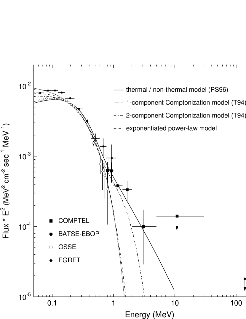
Figure 6: Contemporaneous broad-band spectrum of Cygnus X-1 including data from COMPTEL, OSSE and BATSE. Also shown are the various model fits, whose parameters are listed in Table 3. The data are plotted in units of $E^{2}$ times the photon flux. For the sake of clarity, upper limits from OSSE and BATSE are not shown, but these are consistent with the total dataset. The EGRET upper limit is based on data from Hartman et al. (1999).

Source geometry is also an important factor that must be considered in the interpretation of broad-band spectra. For example, Haardt et al. (1993) argued, based on Monte Carlo studies, that improved fits to broad-band spectra could be achieved by incorporating a reflection component along with the inverse Compton component. The reflection component would result from the Compton scattering of hard X-rays from an accretion disk corona off a cool optically-thick accretion disk. The reprocessing leads to an enhancement of emission in the 10–100 keV energy range. The requirement for such a reprocessed component is also supported by the observation of a fluorescence line from neutral iron (e.g., Ebisawa et al., 1996). Assuming a geometry consisting of an optically thin corona above an optically-thick accretion disk, Haardt et al. (1993) showed that the model was consistent with data from EXOSAT, SIGMA (Salotti et al., 1992) and OSSE (Grabelsky et al., 1993), suggesting a much higher coronal electron temperature ($kT_{e}\sim 150$ keV) and an even smaller optical depth ($\tau\sim 0.3$) than suggested by Comptonization models alone. The reflection component was also incorporated into an accretion disk corona (ADC) model by Dove et al. (1997). In this case, the geometry consisted of a hot inner spherical corona with an exterior accretion disk. Reasonable comparisons with the broad-band spectrum from 1 keV up to several hundred keV were demonstrated with an electron temperature of $kT_{e}\sim 90$ keV and an optical depth of $\tau\sim 1.5$. A similar model was used by Gierlinski et al. (1997) to fit a combined Ginga-OSSE spectrum, but they found that, with fixed normalization between the Ginga and OSSE spectra, a second Comptonization component was needed to improve the fit at the highest energies. (It has been pointed out by Poutanen (2000), however, that a single temperature Comptonization model fits the Ginga-OSSE data quite well if the relative normalization between the two spectra is left as a free parameter; see Figure 6 of Poutanen (1998).) Moskalenko, Collmar & Schönfelder (1998) also developed a multi-component model to explain the spectrum from soft X-rays into the $\gamma$-ray region. In this case, a central spherical corona surrounds the black hole itself, outside of which is the optically-thick accretion disk, with a much hotter outer corona surrounding the entire system.

The use of two-component Comptonization models to improve spectral fits is motivated by the reasonable assumption that the Comptonization region will not be isothermal. A simple two-temperature model may not be very physical, however, since it implicitly assumes that there are two distinct non-interacting regions in which Comptonization is taking place. A more realistic approach would be to assume a continuum of Comptonization parameters. Skibo & Dermer (1995) argued that a thermally-stratified black hole atmosphere could act to harden the spectrum. They simulated a model involving a high-energy spherical core surrounded by an optically thick accretion disk. If the inner core of the high-energy region were hot enough, then a hard tail extending into the MeV region might be produced. A similar model was used to interpret the first combined spectral results from the BATSE and COMPTEL experiments on CGRO (Ling et al., 1997) . Thermal stratification is also an essential concept in the transition disk model of Misra & Melia (1996). This model involves large thermal gradients in the inner region of an optically thick accretion disk. These gradients represent a transition between the cold optically thick disk and the hot plasma which exists near the inner part of the disk. This model has been used to provide a good fit to spectra in the 2–500 keV energy band (Misra et al., 1997, 1998). Dove et al. (1997) also incorporated thermal stratification into the structure of the inner corona of their model.

The net effect of thermal gradients is to produce a non-Maxwellian electron energy distribution. A high energy tail in the electron distribution leads, via the the inverse Compton process, to a high energy tail in the photon distribution. Several models have sought to explain hard-tail emissions by invoking some kind of nonthermal process to generate a high energy (possibly relativistic) tail to the thermal Maxwellian electron energy distribution. Many of these hybrid thermal/non-thermal models (e.g., Bednarek et al., 1990; Crider et al., 1997; Gierlinski et al., 1997; Poutanen, 1998; Poutanen & Coppi, 1998; Coppi, 1999) tend to be rather ad hoc, in that they assume some accelerated (or non-Maxwellian) particle population and then proceed to explore the subsequent consequences. Typically, although not always, the nonthermal population takes the form of a power-law in the electron energy distribution. Such a distribution is similar to that seen, for example, in solar flares (e.g., Coppi, 1999). Both Crider et al. (1997) and Poutanen & Coppi (1998) have shown that a Maxwellian plus power-law form for the electron energy distribution can be adapted to fit a composite COMPTEL-OSSE spectrum of Cygnus X-1.

Others have considered physical mechanisms by which non-thermal electron distributions might be developed. For example, both stochastic particle acceleration (Dermer, Miller, & Li, 1996; Li, Kusunose & Liang, 1996) and MHD turbulence (Li & Miller, 1997) have been proposed as mechanisms for directly accelerating the electrons. The ion popoulation might also contribute to the non-thermal electron distribution in the case where a two-temperature plasma develops (e.g., Dahlbacka et al., 1974; Shapiro, Lightman and Eardley, 1976; Chakrabarti & Titarchuk, 1995). In this situation, the ion population may reach a temperature of $kT_{i}\sim 10^{12}$ K, resulting in $\pi^{o}$ production from proton-proton interactions (e.g., Eilik, 1980; Eilik & Kafatos, 1983). The $\pi^{o}$ component then leads, via photon-photon interactions between the $\pi^{o}$-decay photons and the X-ray photons, to production of energetic (nonthermal) $e^{+}-e^{-}$ pairs. Jordain & Roques (1994) used this concept to fit the hard X-ray tails of not only Cygnus X-1, but also GRO J0422+32 and GX 339-4, as measured by both SIGMA and OSSE. While retaining the standard ST80 spectrum to explain the emission at energies below 200 keV, they used $\pi^{o}$ production to generate the nonthermal pairs needed to fit the spectrum at energies above $\sim 200$ keV.

The history of Cygnus X-1 is also riddled with unconfirmed reports of very intense, very broad line emission in the region around 1 MeV, far exceeding that which would be expected from a simple extrapolation of the low energy continuum spectrum (e.g., Ling et al., 1987; McConnell et al., 1989; Owens & McConnell, 1992). The broad MeV feature observed by HEAO-3 (Ling et al., 1987) occured under an unusual source condition when both the hard and soft X-ray fluxes were low. Liang & Dermer (1988) interpreted the feature as evidence for the presence of a very hot ($kT_{e}\sim 400$ keV) pair-dominated cloud in the inner region of the accretion disk. In this model, pairs may escape the system and produce a weak narrow annihilation feature in the cold surrounding medium (Dermer & Liang, 1989). Such a feature was also suggested in the HEAO-3 spectrum (Ling & Wheaton, 1989). Melia & Misra (1993) extended this model by considering a more realistic thermally stratified cloud. These “MeV bumps,” have not been seen by any of the experiments on the Compton Gamma-Ray Observatory (CGRO) (McConnell et al., 1994; Phlips et al., 1996; Ling et al., 1997). Any such emission must therefore be time-variable (c.f., Harris et al., 1993).

Although there have been no recent observations of an “MeV bump” in the spectrum of Cygnus X-1, the continuum flux levels that are now generally observed around 1 MeV still indicate a substantial hardening of the high energy spectrum. The extent to which the spectrum hardens at energies approaching 1 MeV has now become an important issue for theoretical modeling of the spectrum. Data from CGRO, in particular the COMPTEL experiment on CGRO, offer the best opportunity for more precisely defining the highest energy parts of the spectrum. Such measurements are critically important in our efforts to determine the nature of the complete hard X-ray / $\gamma$-ray spectrum.

In this paper, we present a composite low X-ray state spectrum of Cygnus X-1 compiled from contemporaneous CGRO observations that spans the energy range from $\sim$30 keV up to $\sim 5$ MeV. This spectrum should add new insights into the modeling of the broad band $\gamma$-ray spectrum of Cygnus X-1 and especially its emissions just above 1 MeV. In $\S$ 2 we briefly describe the COMPTEL experiment, the data from which have been the focus of this investigation. The observations and data selection are described in $\S$ 3. In $\S$ 4 we discuss the analysis of the COMPTEL data. The analysis is expanded in $\S$ 5 to include data from both OSSE and BATSE. A discussion of the results is then presented in $\S$ 6.

2 The COMPTEL Experiment

The COMPTEL experiment images 0.75–30 MeV $\gamma$-radiation within a field-of-view of $\sim 1$ sterdian. It consists of two independent layers of detector modules separated by 150 cm. The upper (D1) layer is composed of 7 independent NE213A liquid scintillator detectors, each 28 cm in diameter and 8.5 cm thick. The lower (D2) layer is composed of 14 independent NaI(Tl) detectors, each 28 cm in diameter and 7.5 cm thick. An event is defined as a coincident interaction in a single D1 detector and a single D2 detector. For each event, the total energy is estimated as the sum of the energy losses in both D1 and D2. The interaction locations in both detectors are determined using the relative responses of the various PMTs which are affixed to each D1/D2 detector. In this manner, the interaction locations can be determined with an uncertainty of about 2.0 cm. The measurement of the time-of-flight (TOF) between D1 and D2 and the pulse-shape (PSD) in D1 allow for the rejection of a large fraction of background events, including both upward-moving and neutron-induced events. A more detailed description of COMPTEL can be found in Schönfelder et al. (1993).

The basic principle of COMPTEL imaging is governed by the physics of Compton scattering. If the energy loss of the Compton scattered electron is completely contained within the D1 module and if the scattered photon is completed absorbed by the D2 module, then we have an accurate measure of both the scattered electron energy and the scattered photon energy. Knowledge about the interaction locations in both the upper (D1) and lower (D2) detector layers provides information about the path of the scattered photon. Without more complete knowledge regarding the direction of the scattered electron, the possible arrival direction of the incident photon is confined to a annular region on the sky. This event circle is defined to have an angular radius ($\bar{\phi}$) determined by the Compton scattering formula:

$$\cos\bar{\phi}=1-{m_{e}c^{2}\over E_{2}}+{m_{e}c^{2}\over{E_{1}+E_{2}}},$$ (1)

where $m_{e}c^{2}$ is the electron rest mass energy and $E_{1}$ and $E_{2}$ are the energy deposits measured in D1 and D2, respectively. The superposition of many event circles can lead to the crude localization of a source by determining the direction in which the majority of the event circles intersect (c.f., Figure 7 of Winkler et al. 1992). In practice, the analysis of COMPTEL data is far more complex. Many instrumental effects complicate this simplified approach. For example, incomplete energy absorption in either D1 or D2 can render equation (1) invalid. Effects such as these are taken into account in the final analysis via an appropriate instrumental point spread function (PSF).

3 The Observations

Since the launch of CGRO in April of 1991, several observations of the Cygnus region have been carried out with COMPTEL. In order to assemble a broad-band picture of the $\gamma$-ray emission from Cygnus X-1, we set out to combine COMPTEL data with data from the BATSE and OSSE experiments on CGRO. The BATSE experiment is an uncollimated array of NaI scintillation detectors covering $4\pi$ steradian and operating in the $\sim$30 keV – 1.8 MeV energy range. The spectral analysis of a given point source is achieved using techniques that rely on the occultation of the source flux by the Earth. There are currently two approaches to spectral analysis with BATSE. The BATSE experiment team routinely uses a technique that uses data only from a limited time period about each Earth occultation (both ingress and egress; Harmon et al. (1992)). Another approach, developed by Ling et al. (1996), makes use of a more extensive set of data in an effort to model the combined effect of some 65 celestial sources of $\gamma$-radiation and various models of the instrumental background. This method of BATSE source analysis is embodied in a software system known as the Enhanced BATSE Occultation Package (EBOP; Ling et al., 1996, 2000). The OSSE experiment is a collimated array of NaI detectors that are used for both on-source and off-source measurements. OSSE operates in the 50 keV – 10 MeV energy range.

In selecting those CGRO observations to use in our broad-band analysis, we required contemporaneous observations by all three instruments (COMPTEL, BATSE and OSSE). The COMPTEL FoV is centered on the CGRO pointing direction (the z-axis) and can generally study sources that are within $40\arcdeg$ of the pointing direction. OSSE has a more limited FoV of $11\arcdeg$ by $4\arcdeg$ and is restricted to pointing directions along the spacecraft X-Z plane. BATSE, on the other hand, can observe Cygnus X-1 continually by means of Earth occultation techniques. The data selection was therefore driven by the availability of contemporaneous COMPTEL and OSSE data. The selection was also confined to the first three cycles of CGRO observations (1991 – 1994), based on the quality of the COMPTEL data that was available at the time this study was undertaken. The initial selection of CGRO observation periods, based on these criteria, is listed in Table 1. In addition to the dates of each observation, the table also gives the COMPTEL viewing angle (the offset angle from the COMPTEL pointing direction) and a crude estimate of COMPTEL’s total effective on-axis exposure to Cyg X-1 (measured in days). The exposure estimate is based on an approximated angular response for COMPTEL and includes estimates for the effects of Earth occultation times and telemetry contact times.

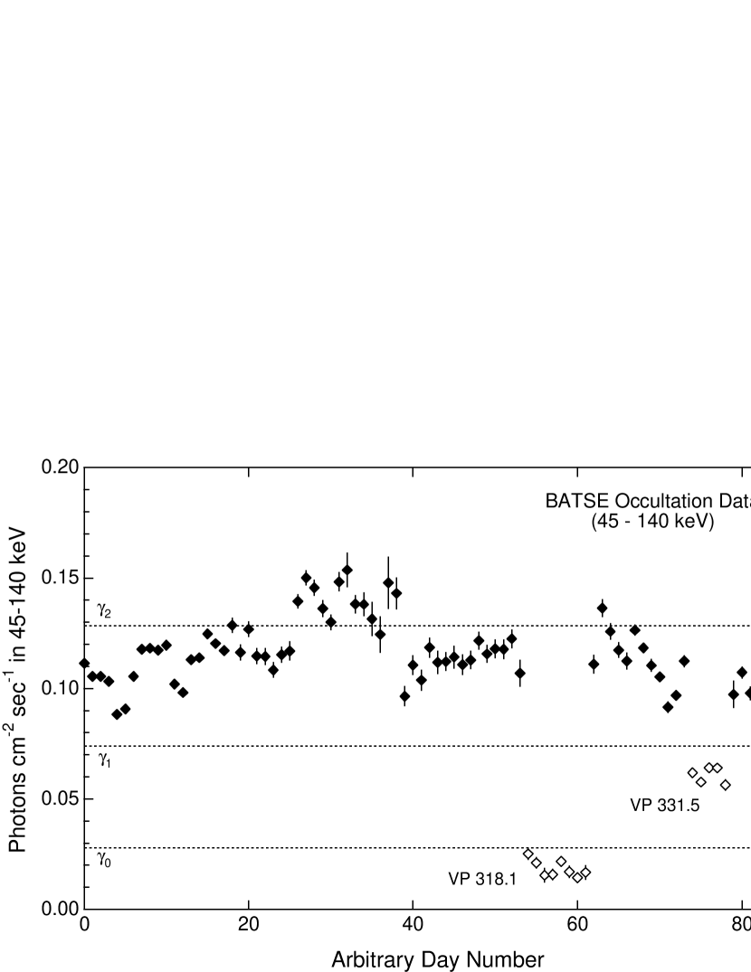
Figure 1: Hard X-ray flux measurements from BATSE occultation data for those days in which COMPTEL observed Cygnus X-1. These data cover the CGRO observations listed in Table 1. The open diamonds are from VP 318.1 and VP 331.5, which were excluded from the final analysis. The hard X-ray flux levels defined by Ling et al. (1987, 1997) are indicated.

The initial analaysis of the broad-band spectrum produced from the full set of observations in Table 1 led to a significant discrepancy between the BATSE and OSSE spectra (McConnell et al., 1998). This has been largely resolved by a further selection based on the hard X-ray flux. Figure 1 shows the hard X-ray flux, as measured by the BATSE occultation technique, during each of the observations in Table 1. These data, taken from the BATSE web site at Marshall Space Flight Center , include statistical errors only. Also indicated in Figure 1 are the $\gamma_{0}$, $\gamma_{1}$, and $\gamma_{2}$ flux levels as defined by Ling et al. (1987, 1997). In general, the hard X-ray flux varied between the $\gamma_{1}$ and $\gamma_{2}$ levels. However, the hard X-ray flux was considerably below-average (at the $\gamma_{0}$ level) during Viewing Period (VP) 318.1 and, to a lesser extent, during VP 331.5. Due to the way that the data were collected, these low hard X-ray flux observations were weighted differently by the various CGRO instruments. These different weightings were directly responsible for the discrepancies noted during our initial analysis. For the final analysis reported here, we excluded the data from VP 318.1 and VP 331.5. The remaining data corresponded to a relatively constant hard X-ray flux of 0.1 photons cm^-2 s^-1 in the 45–100 keV energy band. It is assumed, based on the consistent level of hard X-ray flux, that the corresponding soft X-ray flux was also consistent during these observations and that these data all correspond to the canonical low X-ray state of Cygnus X-1. During the first few months of the CGRO mission (from the launch in April of 1991 until October of 1991) all-sky monitoring data from Ginga (1–20 keV) is available that confirms our assumption that Cygnus X-1 was in its low state (Kitamoto et al., 2000). For the period from October of 1991 until December of 1995 (when RXTE was launched), the data archives at the High Energy Astrophysics Science Archive Research Center (HEASARC) show only sporadic pointed observations by ASCA or ROSAT, none of which correspond precisely to any of the COMPTEL observation times.

4 COMPTEL Data Analysis

The analysis of COMPTEL data can be logically divided into a spatial (or imaging) analysis and a spectral analysis. In practice, however, the spatial and spectral analysis of the data is inextricably linked via the PSF and its dependence on the incident photon spectrum. The goal of the spatial analysis is to define, for a given range of photon energy loss values, the corresponding photon intensity distribution on the sky. The final source spectrum is then derived, in a self-consistent manner, from the results of a spatial analysis in several distinct energy loss intervals.

4.1 Event Selections and the COMPTEL Dataspace

The spatial analysis is performed by first selecting data within some range of measured (total) energy loss values. Within the chosen energy range, events are carefully selected in order to reduce the background contributons and to maximize the signal-to-noise. These event selections include the following: a) restrictions on D1 pulse shape (PSD) to select only those events consistent with incident photons; b) a TOF selection to reject all but “forward” scattered photon events; c) a scatter angle ($\bar{\phi}$) selection to restrict the analysis to a range of values which is dominated by source events rather than by background events; and d) a selection to reject any event whose event circle passes within $10\arcdeg$ of the Earth’s disk (thus minimizing the background of earth albedo $\gamma$-rays).

Once the event data have been selected, the subsequent analysis is carried out within a three-dimensional dataspace that is defined by the fundamental quantities that represent each COMPTEL event. The first two of these parameters, the angles that are arbitarily referred to as $\chi$ and $\psi$, define the direction of the photon that is scattered from D1 to D2. The third parameter defining this dataspace is the Compton scatter angle ($\bar{\phi}$), as estimated from equation (1) using the measured energy losses in both D1 and D2.

For a point source, the distribution of events in the 3-dimensional ($\chi$, $\psi$, $\bar{\phi}$) dataspace is generally contained within the interior of a cone whose apex corresponds to the direction of the source. This distribution corresponds to the PSF of COMPTEL. The details of the PSF depend not only on the energy range of the analysis, but also on the shape of the assumed input spectrum, especially as it extends to higher energies. In the present analysis, we have derived PSFs from Monte Carlo simulations (Stacy et al., 1996). The current uncertainties in the PSF are estimated to contribute a systematic error of not more than $\sim$15–20% to the flux uncertainties. This error is dominated by uncertainties in the physical modeling of COMPTEL and not by Monte Carlo statistics.

4.2 COMPTEL Spatial Analysis (Imaging)

The derivation of an image from binned COMPTEL event data (binned into the three-dimensional dataspace) starts by folding an assumed source distribution through the instrumental response (PSF). The PSF incorporates all of the various physical processes alluded to in $\S$ 2 as well as the various event selections which have been imposed on the data. The known exposure and geometric factors (which are specific to a given observation and include, for example, the on/off status of the various modules) are then included. Finally, a ‘background’ model, which may consist of several components, is added in. This process results in an estimate of the event distribution in the three-dimensional COMPTEL dataspace, which can be compared directly with the real data. Subsequent iterations of this process lead to a more precise estimate of the source distribution on the sky.

In practice, the imaging analysis of the COMPTEL data is performed in one of two ways. One technique employs the maximum entropy method to derive a source distribution on the sky (Strong et al., 1992; Schönfelder et al., 1993). As presently implemented for COMPTEL data analysis, this algorithm does not provide quantitative error estimates. A more quantitative analysis can be made using a maximum likelihood technique (de Boer et al., 1992; Schönfelder et al., 1993). This approach compares the relative probability of a model which contains only background to the probability of a model which contains both the background plus a single point source at the given location (the likelihood ratio). This method provides quantitative information regarding both the source location and the flux together with their associated errors.

The background model used to generate an image is a crucial component of the analysis. These background models consists of components which describe both the (internal) instrumental background and the (external) sky background. The term ’background’, in this case, refers to all photon sources other than the source of interest (Cygnus X-1). To date, the most successful approach for estimating the instrumental background involves a smoothing technique which suppresses point-source signals while preserving the general background structure (Bloemen et al., 1994). The sky background component typically includes both known (or suspected) point sources and diffuse sources (such as the galactic diffuse emission). The maximum likelihood analysis provides a best-fit normalization factor (and associated uncertainty) for each background component.

The location of Cygnus X-1 in galactic coordinates ($l=71.3\arcdeg,b=3.1\arcdeg$) places it in a rather complex region. The background modeling therefore included a number of different models for the spatial distribution of the celestial photon emission. These models corresponded either to established models for celestial $\gamma$-ray emission (e.g., models based on the distribution of atomic and molecular gas within the galaxy) or on ad-hoc photon distributions as derived directly from COMPTEL images. Images were generated using a variety of such models in various combinations. In all cases, a point source model at the location of Cygnus X-1 was included. The resulting distribution of flux values for the Cygnus X-1 point source model provides a direct measure of the errors in the point source analysis, incorporating both the statistical errors from counting statistics and the systematic errors introduced by the background modeling.

For the purposes of background modeling, there are two known sources of $\gamma$-ray emission that should be noted. The first of these is the diffuse $\gamma$-ray emission from the galaxy. We have made use of a model that is consistent with global studies of COMPTEL data (e.g., Strong et al., 1996; Bloemen et al., 1999, 2000). This model includes estimates of the $\gamma$-ray emission which results from the interaction of cosmic rays with both $HI$ and $H_{2}$, as well as the contribution from inverse Compton emission off cosmic ray electrons (Strong & Youseffi, 1995; Strong et al., 1996; Strong, Moskalenko, & Reimer, 2000). An $E^{-2}$ power law spectrum is assumed for the diffuse $\gamma$-ray spectrum. A second known source of $\gamma$-ray emission is the 39.5 msec pulsar PSR 1951+32, which lies only $2.8\arcdeg$ from Cygnus X-1 (at galactic coordinates $l=68.8\arcdeg,b=2.8\arcdeg$). Although not readily apparent in spatial studies, a timing analysis of COMPTEL data integrated over the full 750 keV to 30 MeV energy band independently provides evidence for PSR 1951+32 (Kuiper et al., 1998). Its close proximity to Cygnus X-1 makes this source an important component of the background models.

A sample of COMPTEL imaging data is shown in Figure 2, where we present a maximum likelihood map derived from data integrated over the energy loss range of 0.75 – 2.0 MeV. The contours represent constant values of the quantity $-2\ln{\lambda}$, where $\lambda$ is the likelihood ratio. In a search for single point sources, $-2\ln{\lambda}$ has a chi-square distribution with 3 degrees of freedom. (For instance, a $3\sigma$ detection corresponds to $-2\ln{\lambda}$ = 13.9.) Cygnus X-1 is clearly visible. The likelihood reaches a value of $-2\ln{\lambda}=93.2$ at the position of Cygnus X-1, which corresponds to a detection significance of $9.7\sigma$. These same data were used to derive the $1\sigma$, $2\sigma$ and $3\sigma$ location confidence contours shown in Figure 3, which demonstrate the ability of COMPTEL to locate the source of emission. In defining constraints on the source location, $-2\ln{\lambda}$ has a chi-square distribution with 2 degrees of freedom. So the $1\sigma$, $2\sigma$ and $3\sigma$ location confidence contours correspond to a change in likelihood of 2.3, 6.2, and 11.8, respectively. The contours reflect only the statistical uncertainties; systematic effects are not included.

4.3 COMPTEL Spectral Analysis

A photon spectrum of Cyg X-1 was assembled using flux values derived from the spatial (imaging) analysis of COMPTEL data in five distinct energy bands. Since the flux measurements are, at some level, dependent on the instrumental PSF (and the spectral form assumed for that PSF), the resulting spectrum is also dependent on the PSF (and the spectral form assumed for that PSF). The analysis therefore included a careful check on the consistency of the resulting photon spectrum with the spectral form assumed in generating each PSF.

Initial fluxes were derived using PSFs based on an $E^{-2}$ power-law spectrum. The resulting photon spectrum was fit with a power-law spectrum of the form,

$${dN\over dE}=AE^{-\alpha}$$ (2)

The fit gave a photon index of $\alpha=-3.2(\pm 0.4)$. This suggested the need to use PSFs based on a steeper power-law source spectrum. Subsequent results were derived using PSFs based on an $E^{-3}$ power-law spectrum. A power-law fit to this second spectrum gave an index of $\alpha=-3.3(\pm 0.4)$. From this result, we conclude that, at least within this range of PSFs, the resulting flux values are relatively insensitive to changes in the PSFs. In other words, the derived photon spectrum is not very compliant with respect to the assumed input spectrum. The robust nature of the extracted photon spectrum means that spectral fits in photon dataspace (rather than energy-loss dataspace) can be performed with a high degree of reliability.

The final flux data points from the analysis of the COMPTEL data are given in Table 2. These results were derived using PSFs based on an $E^{-3}$ power-law spectrum. The quoted uncertainties include both statistical and systematic errors. The statistical errors are those due to the counting statistics of the measurement. The systematic errors are based on results from using various background models (as described in $\S$ 4.2) and, in some cases, are comparable to the statistical errors, especially at lower energies. (We have not included here the systematic error associated with the PSF calculations, as discussed in $\S$ 4.1, because these are considered to be negligible relative to other sources of error.)

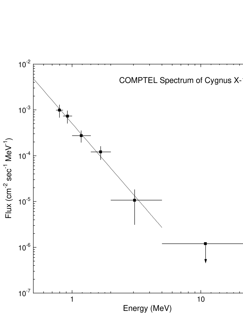
Figure 4: The photon spectrum of Cygnus X-1 as derived from COMPTEL data, along with the best-fit power-law (with a spectral index of $\alpha=-3.3$). This spectrum corresponds to the data in Table 2.

A plot of the COMPTEL spectra, along with the best-fit power-law fit, is shown in Figure 4. The best-fit power-law gives a spectral index ($\alpha$) of $-3.3\pm 0.4$ and an amplitude of $5.1(\pm 0.8)\times 10^{-4}$ cm^-2 s^-1 MeV^-1 at 1 MeV. These data provide convincing evidence for emission up to 2 MeV, with a marginal detection in the 2–5 MeV energy band. There is no evidence for emission at energies above 5 MeV. These conclusions are supported by the images generated from these same data. The resulting flux values are consistent with previously published results (e.g., McConnell et al., 1994).

5 Broad-Band CGRO Spectral Analysis

Several different models can be used to fit the COMPTEL data, but the lack of low energy data points results in very poor constraints on the model parameters. We therefore must incorporate additional spectral data (at lower energies) in order to more precisely define the broad-band spectrum and hence gain some important insight into the physics of the emission region. The additional data used in this case are the contemporaneous BATSE and OSSE data. As previously discussed, these data have been selected based both on the requirement of contemporaneous observations and on the requirement of a consistent level of hard X-ray flux.

For these broad-band spectra, power-law models clearly do not provide an adequate description of the data. We chose four alternative spectral forms to help describe the data. The first form is an exponentiated power-law,

$${dN\over dE}=AE^{-\alpha}e^{-E/{E_{c}}}$$ (3)

This particular function, defined by a power-law index ($\alpha$) and a characteristic energy cutoff ($E_{c}$), is not based on any underlying physical model, but its functional form approximates the spectrum at these energies (e.g., Phlips et al., 1996). The data was also fit using both single-component and two-component Comptonization models. In this case, we used the analytical Comptonization model of Titarchuk (1994), which is characterized by a normalization factor, an electron temperature ($kT_{e}$) and an optical depth ($\tau$). A fourth functional form is the hybrid thermal/non-thermal model of Poutanen & Svensson (1996) (see also Poutanen, 1998; Poutanen & Coppi, 1998), which describes the photon spectrum resulting from a thermal (Maxwellian) electron distribution plus a non-thermal (power-law) electron distribution at higher energies. The thermal component is described by a characteristic temperature ($kT_{e}$). The non-thermal component is characterized as a power law with spectral slope $p_{e}$ extending from an electron Lorentz factor $\gamma_{min}$ (where the Maxwellian transforms to the power-law tail) up to a Lorentz factor of $\gamma_{max}=1000$. The electron population is assumed to reside in a accretion disk corona with an optical depth of $\tau$. This particular model is useful in that it permits a quantitative description of the underlying electron distribution.

We have already demonstrated that the reproduced COMPTEL spectrum is relatively insensitive to the shape of the assumed spectrum, thus giving us some level of confidence in fitting these data in photon-space. Here we also make the same assumption with regards to both the BATSE and OSSE spectra. Given the steepness of the measured spectra, this assumption is likely to be a safe one, at least to first-order. This approach greatly simplifies the analysis using multiple observations from multiple experiments.

The initial fits to the combined datasets were performed over the 50 keV to 5 MeV energy range. A significant amount of scatter in the OSSE and BATSE data at energies below 200 keV led to rather poor chi-square values for the resulting fits. In order to obtain improved chi-square values, the final model fits were derived from the data between 200 keV and 5 MeV. In addition to the reduced scatter of the BATSE and OSSE data, the general agreement of these two datasets was also much improved at energies above 200 keV. Below 200 keV, there exists discrepancies of up to 25% between the BATSE and OSSE data, whereas at energies above 200 keV the spectra were found to agree quite closely, with differences typically less than 5%. This range is also above the range where many models predict the presence of a backscatter component from photons scattering off a cooler optically thick accretion disk. Spectral fits were derived by allowing both the BATSE and OSSE normalizations to be free parameters. We found that constraining the COMPTEL normalization to that of either BATSE or OSSE gave consistent results for the physical parameters of interest. The final fit parameters were derived by constraining the COMPTEL normalization to that of OSSE.

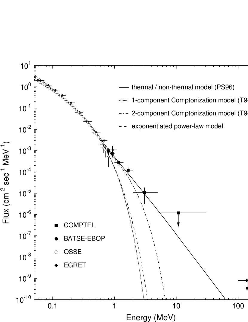
Figure 5: Contemporaneous broad-band spectrum of Cygnus X-1 including data from COMPTEL, OSSE and BATSE. Also shown are the various model fits, whose parameters are listed in Table 3. The data are plotted in units of photon flux. For the sake of clarity, upper limits from OSSE and BATSE are not shown, but these are consistent with the total dataset. The EGRET upper limit is based on data from Hartman et al. (1999).

A summary of the broad-band fit results is given in Table 3. The broad-band photon spectrum, along with the various spectral fits, is shown in Figure 5. The same data is also shown in Figure 6, but now plotted in terms of $E^{2}$ times the photon flux; this plot shows that the power peaks around 100 keV and also accentuates the differences between the spectra and the various model fits. In addition, we also plot (in both Figures 4 and 5) an estimated upper limit from EGRET data collected during Cycles 1–4 of the CGRO mission, an exposure which is similar to that for the other data included in this analysis. This upper limit is based on data from Hartman et al. (1999) and assumes an $E^{-3}$ source spectrum. These data do not provide any evidence for a cutoff to the high energy power-law.

6 Discussion

We have assembled a broad-band $\gamma$-ray spectrum of Cygnus X-1 using data collected from COMPTEL, BATSE and OSSE during the first three years of the CGRO mission. The data were collected contemporaneously and selected so as to have a common level of hard X-ray flux. The hard X-ray flux during these observations varied between the $\gamma_{1}$ and $\gamma_{2}$ levels of Ling et al. (1987, 1997). Although there is poor coverage at soft X-ray energies during this time frame, data from both BATSE (Ling et al., 1997) and OSSE (Phlips et al., 1996) indicate that, for the included observations (Table 1), the hard X-ray / $\gamma$-ray spectrum remained fairly stable. In particular, the spectral form is that of the “breaking $\gamma$-ray state”, as defined by Grove et al. (1998), which is generally associated with the low X-ray state. (McConnell et al. (2000) compare the spectrum presented here with that obtained during a high X-ray state observation in 1996, showing evidence for spectral variability at MeV energies.)

The COMPTEL data provide evidence of significant emission out to at least 2 MeV. There is additional, but perhaps less compelling, evidence for emission in the 2–5 MeV energy band, with no evidence for emssion above 5 MeV. An analysis of the COMPTEL data alone does not adequately constrain the nature of the broad-band $\gamma$-ray spectrum. A more complete interpretation of the COMPTEL data requires the consideration of the spectrum at lower energies. Here we have used contemporaneous data from both BATSE and OSSE to define the spectrum at lower energies.

As noted previously (McConnell et al., 1994), these data do not provide any evidence for an “MeV bump”. The spectrum above 750 keV can be described as a power-law with a photon spectral index of $\alpha$ = -3.2. There is no evidence for a break in this power-law. An estimated upper limit from EGRET data does not constrain the extrapolated power-law. An important goal of future measurements will therefore be the determination of the break energy of this power-law spectrum.

Broad-band spectral fits, at energies above 200 keV, show that both the single-component Comptonization model and the exponentiated power-law model do not provide a good fit to the data at energies above 1 MeV, although they do provide very good fits to the BATSE-OSSE data alone. The COMPTEL data dictate the need for an additional spectral component. The high energy fit is significantly improved using a two-component Comptonization model. Unfortunately, the analytical model (T94) begins to fail in this case, because the derived electron temperature of the high-temperature component exceeds the range that is generally allowed for this model (Skibo et al., 1995). Nonetheless, the improvements that result from the two-component Comptonization model suggest that perhaps a stratified Comptonization region (providing a range of both electron temperatures and optical depths) would be more appropriate for modeling the spectrum. Ling et al. (1997) reached the same conclusions based on Monte Carlo modeling of BATSE spectra combined with (non-contemporaneous) COMPTEL data (McConnell et al., 1994). Physically, this is a much more appealing concept than that of a multi-component Comptonization model in which there is no interaction between isothermal Comptonization regions. Thermal gradients are incorporated into several models, all of which lead to the generation of a high energy tail (e.g., Skibo & Dermer, 1995; Chakrabarti & Titarchuk, 1995; Misra & Melia, 1996; Ling et al., 1997).

Hybrid thermal/nonthermal models may also be a viable possibility for explaining the observed $\gamma$-ray spectrum. The existence of such distributions is clearly established in the case of solar flares (e.g., Coppi, 1999) and it is therefore natural to expect that similar distributions exist elsewhere in the universe. Several such models have been discussed in the literature (e.g., Crider et al., 1997; Gierlinski et al., 1997; Poutanen & Svensson, 1996; Poutanen, 1998; Poutanen & Coppi, 1998; Coppi, 1999). Fits to our broad-band spectrum using the model of Poutanen & Svensson (1996) provide a quantitative estimate of the electron distribution. In this case, the spectral data can be explained by a thermal Maxwellian distribution with an electron temperature of $kT_{e}=86$ keV, coupled to a power-law electron spectrum with a power-law index of $p_{e}=4.5$. The transition between the Maxwellian and the power-law occurs at an electron kinetic energy of $\sim 570$ keV ($\gamma_{min}=2.12$). The electron population is embedded in an accretion disk corona with an optical depth of $\tau=1.63$. The derived spectral index for the power-law tail is somewhat harder (4.5 versus 3.2) but still consistent with that derived by Crider et al. (1997).

The role of $\pi^{o}$-production can also not be ruled out as a contribution to the measured spectrum. As initially proposed by Jordain & Roques (1994), this mechanism was used to explain the inadequacy of the ST80 model at energies below 1 MeV. It has not been applied to Cygnus X-1 at energies above 1 MeV, which would be required to test this model with the present results. Models for advection-dominated accretion flows (ADAF) predict ion temperatures of $\sim 10^{12}$ K in the inner part of the accretion flow (e.g., Chakrabarti & Titarchuk, 1995), suggesting the possibility of pion production (although it is not clear whether an ADAF is present during the low X-ray state of Cygnus X-1).

The spectrum presented here clearly indicates the need for a non-Maxwellian electron energy distribution. In particular, it strongly suggests the presence of a high energy tail to that distribution. Whether this results from thermal gradients or from a more isothermal system coupled with a non-thermal component remains an open question. The shape of the electron distribution and its high energy tail can only be determined by measurements that extend into the MeV energy region.

There have been several studies of the broad-band hard X-ray emission from Cygnus X-1 based, in part, on OSSE data. These studies have concentrated on joint observations with lower energy experiments, such as GINGA, ASCA or RXTE. Since these observations are of relatively short duration, these spectra typically do not exhibit a well-defined hard tail due to limited statistics near 1 MeV. Nonetheless, the presence of a hard tail in the continuum emission near 1 MeV now appears to be well-established. An excess above the standard Comptonization models has been discussed several times in the literature for both Cygnus X-1 (e.g., McConnell et al., 1994; Phlips et al., 1996; Ling et al., 1997) and for GRO J0422+32 (van Dijk et al., 1995). The data presented here provide the best quantitative measurement of the spectrum of Cygnus X-1 at these energies and thus provide the best opportunity to study the nature of this hard tail emission. The IBIS and SPI instruments on INTEGRAL will provide only a marginal improvement in the continuum sensitivity over that of CGRO (Lichti et al., 1996; Ubertini et al., 1996). In addition, with their much smaller FoV, the INTEGRAL instruments, unlike COMPTEL, may be severely limited in terms of their total exposure to Cygnus X-1. COMPTEL may therefore provide the best available data on the MeV spectrum of Cygnus X-1 for many years to come. The continued analysis of data from CGRO (only a fraction of the total COMPTEL data are used here) may help to further clarify the nature of this high energy emission and perhaps enable us to more fully elucidate the physics of the accretion process around stellar-mass black holes.

Figure 2: COMPTEL maximum likelihood map of the Cygnus region as derived from data accumulated over the energy range from 0.75 to 2.0 MeV. The contour levels start at a likelihood value of 2 with an increment of 12.

Figure 3: COMPTEL location confidence contours for Cygnus X-1 based on the maximum likelihood map in Figure 2. The diamond ($\blacklozenge$) indicates the location of Cygnus X-1 ($l=71.3\arcdeg,b=3.1\arcdeg$). The triangle ($\blacktriangle$) indicates the location of PSR1951+32 ($l=68.8\arcdeg,b=2.8\arcdeg$), a source which has been detected in a COMPTEL timing analysis (Kuiper et al., 1998)

.

Table 1: Relevant CGRO Viewing Periods

Viewing	Start	Start	End	End	Viewing	Effective	Used in
Period	Date	TJD	Date	TJD	Angle	Exposure	Analysis?
2.0	30-May-1991	8406	8-Jun-1991	8415	$1.7^{\circ}$	3.65	yes
7.0	8-Aug-1991	8476	15-Aug-1991	8483	$11.2^{\circ}$	2.72	yes
203.0	1-Dec-1992	8957	8-Dec-1992	8964	$7.0^{\circ}$	1.75	yes
203.3	8-Dec-1992	8964	15-Dec-1992	8971	$7.0^{\circ}$	1.75	yes
203.6	15-Dec-1992	8971	22-Dec-1992	8978	$7.0^{\circ}$	1.69	yes
212.0	9-Mar-1993	9055	23-Mar-1993	9069	$15.4^{\circ}$	2.71	yes
318.1	1-Feb-1994	9384	8-Feb-1994	9391	$4.5^{\circ}$	1.78	no
328.0	24-May-1994	9496	31-May-1994	9503	$7.0^{\circ}$	1.56	yes
331.0	7-Jun-1994	9510	10-Jun-1994	9513	$7.0^{\circ}$	0.95	yes
331.5	14-Jun-1994	9517	18-Jun-1994	9521	$7.0^{\circ}$	1.34	no
333.0	5-Jul-1994	9538	12-Jul-1994	9545	$7.0^{\circ}$	1.86	yes

Table 2: COMPTEL Flux Measurements for Cygnus X-1.

Energy	Counts in	Source	Flux
(MeV)	Dataspace	Counts	(cm-2 s-1 MeV-1)
0.75 – 0.85	63,507	$943\pm 298$	$9.8(\pm 3.1)\times 10^{-4}$
0.85 – 1.0	145,197	$1807\pm 572$	$7.2(\pm 2.3)\times 10^{-4}$
1.0 – 1.4	372,823	$2619\pm 775$	$2.7(\pm 0.8)\times 10^{-4}$
1.4 – 2.0	452,226	$2281\pm 760$	$1.2(\pm 0.4)\times 10^{-4}$
2.0 – 5.0	829,813	$1186\pm 835$	$1.1(\pm 0.8)\times 10^{-5}$
5.0 – 30.0	219,916	$331\pm 345$	$3.9(\pm 4.0)\times 10^{-7}$

Table 3: Spectral Fit Summary (200 keV – 5 MeV)

Exponential Power-Law Model (with 90% confidence limits)
$\alpha$	$1.71^{+.26}_{-.27}$
$E_{c}$ (keV)	$200^{+37}_{-32}$
Red Chi-Square ($\chi^{2}_{\nu}$)	1.53
Degrees of Freedom ($\nu$)	23
One-Component Comptonization Model (with 90% confidence limits)
$kT$ (keV)	$127^{+45}_{-25}$
$\tau$	$0.32^{+.18}_{-.16}$
Red Chi-Square ($\chi^{2}_{\nu}$)	1.67
Degrees of Freedom ($\nu$)	23
Two-Component Comptonization Model (best-fit parameters only)
$kT_{1}$ (keV)	340
$\tau_{1}$	0.30
$kT_{2}$ (keV)	72
$\tau_{2}$	0.81
$A_{1}/A_{2}$	.012
Red Chi-Square ($\chi^{2}_{\nu}$)	0.90
Degrees of Freedom ($\nu$)	19
Hybrid Thermal / Non-Thermal Model (with 90% confidence limits)
$kT_{e}$ (keV)	$86^{+18}_{-8}$
$p_{e}$	$4.50^{+.82}_{-.96}$
$\gamma_{min}$	$2.12^{+.79}_{-.49}$
$\tau$	$1.63^{+1.15}_{-.57}$
Red Chi-Square ($\chi^{2}_{\nu}$)	0.83
Degrees of Freedom ($\nu$)	21

References

- Bednarek et al. (1990) Bednarek, W., et al. 1990, A&A, 236,175
- Bloemen et al. (1994) Bloemen, H., et al. 1994, ApJS, 92, 419
- Bloemen et al. (1999) Bloemen, H., et al., 1999, Astrophys. Lett. & Comm., 39, 205
- Bloemen et al. (2000) Bloemen, H., et al. 2000, in Proceedings of the Fifth Compton Symposium (AIP Conf. Proc. 510), ed. M. L. McConnell & J. M. Ryan (New York: American Institute of Physics), in press
- de Boer et al. (1992) de Boer, H., et al. 1992, Proc. 4th International Workshop on ’Data Analysis in Astronomy’, Erice, Italy (Plenum Press), p. 241
- Chakrabarti & Titarchuk (1995) Chakrabarti, S. K., & Titarchuk, L. G. 1995, ApJ, 455, 623
- Crider et al. (1997) Crider, A., Liang, E. P., Smith, I. A., Lin, D., & Kusnose, M. 1997, in Proceedings of the Fourth Compton Symposium (AIP Conf. Proc. 410), ed. C. D. Dermer, M. S. Strickman, & J.D. Kurfess (New York: American Institute of Physics), p. 868
- Coppi (1999) Coppi, P.S. 1999, in High Energy Processes in Accreting Black Holes (ASP Conf. Ser. 161), ed. J. Poutanen & R. Svensson (San Francisco: ASP), p. 375.
- Dahlbacka et al. (1974) Dahlbacka, G. H., Chapline, G. F., & Weaver, T. A. 1974, Nature, 250, 36
- Dermer & Liang (1989) Dermer, C. D., & Liang, E. P. 1989, ApJ, 339, 512
- Dermer, Miller, & Li (1996) Dermer, C. D., Miller, J. A., & Li H. 1996, ApJ, 456, 106.
- van Dijk et al. (1995) van Dijk, R., et al. 1995, A&A, 296, L33
- Dove, Wilms & Begelman (1997) Dove, J. B., Wilms, J., & Begelman, M. C. 1997, ApJ, 487, 747
- Dove et al. (1997) Dove, J. B., et al. 1997, ApJ, 487, 759
- Ebisawa et al. (1996) Ebisawa, K., Ueda, Y., Inoue, H., Tanaka, Y., & White, N. E. 1996, ApJ, 467, 419
- Eilik (1980) Eilik, J. 1980, ApJ, 236, 664
- Eilik & Kafatos (1983) Eilik, J., & Kafatos, M. 1983, ApJ, 271, 804
- Gierlinski et al. (1997) Gierlinski, M., Zdziarski, A. A., Done, C., Johnson, W. N., Ebisawa, K., Ueda, Y., Haardt, F., & Phlips, B. F. 1997, MNRAS, 288, 958
- Grabelsky et al. (1993) Grabelsky, D. A., et al. 1993, in Compton Gamma-Ray Observatory (AIP Conf. Proc. 280), ed. M. Friedlander, N. Gehrels, & D. J. Macomb (New York; American Institute of Physics), p. 345
- Grebenev et al. (1993) Grebenev, S., et al. 1993, A&AS, 97, 281
- Grove et al. (1998) Grove, J. E., Johnson, W. N., Kroeger, R. A., McNaron-Brown, K., Skibo, J. G., & Phlips, B. F. 1998, ApJ, 500, 899
- Haardt et al. (1993) Haardt, F., Done, C., Matt, G., & Fabian, A. C. 1993, ApJ, 411, L95
- Harmon et al. (1992) Harmon, B. A., et al. 1992, in NASA CP-3137, Compton Observatory Science Workshop, ed. C. R. Shrader, N. Gehrels, & B. Dennis (Washinton, DC: NASA), 69
- Harris et al. (1993) Harris, M. J., Share, G. H., Leising, M. D., & Grove, J. E. 1993, ApJ, 416, 601
- Hartman et al. (1999) Hartman, R. C., et al. 1999, ApJS, 123, 79
- Hua & Titarchuk (1995) Hua, X. M., & Titarchuk, L. 1995, ApJ, 449, 188
- Jordain & Roques (1994) Jourdain, E., & Roques, J. P. 1994, ApJ, 426, L11
- Kitamoto et al. (2000) Kitamoto, S., Egoshi, W., Miyamoto, S., Tsunemi, H., Ling, J. C., Wheaton, W. A., & Paul, B. 2000, ApJ, 531, 546
- Kuiper et al. (1998) Kuiper, L., Hermsen, W., Bennett, K., Carramiñana, A., McConnell, M., & Schönfelder, V. 1998, A&A, 337, 421
- Li & Miller (1997) Li, H., & Miller, J. A. 1997, ApJ, 478, L67
- Li, Kusunose & Liang (1996) Li, H., Kusunose, M., & Liang, E. P. 1996, ApJ, 460, L29
- Liang & Nolan (1983) Liang, E. P., & Nolan, P. L. 1983, Space Sci. Rev., 38, 353
- Liang & Dermer (1988) Liang, E. P., & Dermer, C. D. 1988, ApJ, 325, L39
- Lichti et al. (1996) Lichti, G. L., et al. 1996, Proc. SPIE, 2806, 217
- Ling et al. (1983) Ling, J. C., Mahoney, W. A., Wheaton, W. A., Jacobsen, A. S., & Kaluzienski, L. 1983, ApJ, 275, 307
- Ling et al. (1987) Ling, J. C., Mahoney, W. A., Wheaton, W. A., & Jacobsen, A. S., 1987, ApJ, 321, L117
- Ling & Wheaton (1989) Ling, J. C., & Wheaton, W. A. 1989, ApJ, 343, L57
- Ling et al. (1996) Ling, J. C., Wheaton, W. A., Mahoney, W. A., Skelton, R. T., Radocinski, R. G., and Wallyn, P. 1996, A&AS, 120, C677
- Ling et al. (1997) Ling, J. C., et al. 1997, ApJ, 484, 375
- Ling et al. (2000) Ling, J. C., et al., 2000, ApJS, 127, 79
- McConnell et al. (1989) McConnell, M. L., et al. 1989, ApJ, 343, 317
- McConnell et al. (1994) McConnell, M. L., et al. 1994, ApJ, 424, 933
- McConnell et al. (1998) McConnell, M. L. et al. 1998, in Proceedings of the Fourth Compton Symposium (AIP Conf. Proc. 410), ed. C. D. Dermer, M. S. Strickman & J. D. Kurfess (New York: American Institute of Physics), p. 829
- McConnell et al. (2000) McConnell, M. L. et al. 2000, in Proceedings of the Fifth Compton Symposium (AIP Conf. Proc. 510), ed. M. L. McConnell & J. M. Ryan (New York: American Institute of Physics), in press
- Melia & Misra (1993) Melia, F., & Misra, R. 1993, ApJ, 411, 797
- Misra & Melia (1996) Misra, R., & Melia, F. 1996, ApJ, 467, 405
- Misra et al. (1997) Misra, R., Chitnis, V. R., Melia, F., & Rao, A. R. 1997, ApJ, 487, 388
- Misra et al. (1998) Misra, R., Chitnis, V. R., & Melia, F. 1998, ApJ, 495, 407
- Moskalenko, Collmar & Schönfelder (1998) Moskalenko, I. V., Collmar, W., & Schönfelder, V. 1998, ApJ, 428, 436
- Nolan et al. (1981) Nolan, P., et al. 1981, Nature, 293, 275
- Nolan & Matteson (1983) Nolan, P., & Matteson, J. L. 1983, ApJ, 265, 389
- Owens & McConnell (1992) Owens, A., & McConnell, M. 1992, Comments Astrophys., 16, 205
- Phlips et al. (1996) Phlips, B., et al. 1996, ApJ, 465, 907
- Poutanen & Svensson (1996) Poutanen, J. & Svensson, R. 1996, ApJ, 470, 249 (PS96)
- Poutanen (1998) Poutanen, J. 1998, in Theory of Black Hole Accretion Disks, eds. M. A. Abramowicz, G. Björnsson & J. E. Pringle (Cambridge Univ. Press: New York), p. 100
- Poutanen & Coppi (1998) Poutanen, J., & Coppi, P. 1998, Physica Scripta, T77, 57
- Poutanen (2000) Poutanen, J. 2000, private communications.
- Priedhorsky, Terrell & Holt (1983) Priedhorsky, W. C., Terrell, J., & Holt, S. S. 1983, ApJ, 270, 233
- Salotti et al. (1992) Salotti, L., et al. 1992, A&A, 253, 145
- Schönfelder & Lichti (1974) Schönfelder, V., & Lichti, G. 1974, ApJ, 192, L1
- Schönfelder et al. (1993) Schönfelder, V., et al. 1993, ApJS, 86, 629
- Shapiro, Lightman and Eardley (1976) Shapiro, S. L., Lightman, A. P., & Eardley, D. M. 1976, ApJ, 204, 187
- Skibo et al. (1995) Skibo, J. G., Dermer, C. D., Ramaty, R., & McKinley, J. M. 1995, ApJ, 446, 86
- Skibo & Dermer (1995) Skibo, J. G., & Dermer, C. D. 1995, ApJ, 455, L25
- Stacy et al. (1996) Stacy, J. G., et al. 1996, A&AS, C120, 691
- Steinle et al. (1982) Steinle, H., et al. 1982, A&A, 107, 350
- Strong et al. (1992) Strong, A. W., et al. 1992, Proc. 4th International Workshop on ’Data Analysis in Astronomy’, Erice, Italy (Plenum Press), p. 251
- Strong & Youseffi (1995) Strong, A. W., & Youseffi, G. 1995, Proc. 24th Internat. Cosmic Ray Conf. (Durban), 3, 48
- Strong et al. (1996) Strong, A. W., et al. 1996, A&AS, 120, C381
- Strong, Moskalenko, & Reimer (2000) Strong, A. W., Moskalenko, I. V., and Reimer, O. 2000, in Proceedings of the Fifth Compton Symposium (AIP Conf. Proc. 510), ed. M. L. McConnell & J. M. Ryan (New York: American Institute of Physics), in press
- Sunyaev & Titarchuk (1980) Sunyaev, R. A., & Titarchuk, L. G. 1980, A&A, 86, 121 (ST80)
- Sunyaev & Trümper (1979) Sunyaev, R. A., & Trümper, J. 1979, Nature, 279, 506
- Titarchuk (1994) Titarchuk, L. 1994, ApJ, 434, 570 (T94)
- Titarchuk & Lyubarskij (1995) Titarchuk, L., & Lyubarskij 1995, ApJ, 450, 876
- Titarchuk & Hua (1995) Titarchuk, L., & Hua, X.-M. 1995, ApJ, 452, 226
- Ubertini et al. (1991a) Ubertini, P., et al. 1991a, ApJ, 366, 544
- Ubertini et al. (1996) Ubertini, P., et al. 1996, Proc. SPIE, 2806, 246
- Ubertini et al. (1991b) Ubertini, P., Bazzano, A., La Padula, C., Manchada, R. K., Polcaro, V. F., Staubert, R., Kendziorra, E., & Perotti, F. 1991b, ApJ, 383, 263
- Winkler et al. (1992) Winkler, C. et al. 1992, A&A, 255, L9
- Zdziarski (1984) Zdziarski, A. A. 1984, ApJ, 283, 842
- Zdziarski (1985) Zdziarski, A. A. 1985, ApJ, 289, 514
- Zdziarski (1986) Zdziarski, A. A. 1986, ApJ, 303, 94
.