The role of Star Formation in the evolution of spiral galaxies

Abstract

Spiral galaxies offer a unique opportunity to study the role of star formation in galaxy evolution and to test various theoretical star formation schemes. I review some recent relevant work on the evolution of spiral galaxies. Detailed models are used for the chemical and spectrophotometric evolution, with metallicity dependent stellar yields, tracks and spectra. The models are “calibrated” on the Milky Way disk and generalised to other spirals with some simple scaling relations, obtained in the framework of Cold Dark Matter models for galaxy formation. The results compare favourably to the main observables of present day spirals, provided a crucial assumption is made: massive disks form their stars earlier than low mass ones. It is not clear whether this picture is compatible with currently popular hierarchical models of galaxy evolution. The resulting abundance gradients are found to be anticorrelated to the disk scalelength, support radially dependent star formation efficiencies and point to a kind of “homologuous evolution” for spirals

1 Introduction

Among the three main ingredients required for galactic evolution studies (stellar evolution data, stellar initial mass function and star formation rate), the star formation rate (SFR) is the most important and the less well understood. Despite more than 30 years of observational and theoretical work, the Schmidt law still remains popular among theoreticians and compatible with most available observations. Up to the mid-90ies, observations revealed features concerning the present status of nearby galaxies, from which their past history had to be derived. Developments in the past few years revealed features of the “global SFR” of the Universe and opened perspectives for seing directly the past SFR history of the various galaxy types.

Among the various galaxy types, the disks of spirals are certainly the ones offering the best opportunities to study star formation, for several reasons: i) with respect to ellipticals, spirals offer more constraints (amounts of gas and SFR, metal abundances in the gas); ii) with respect to irregulars, spirals present gradients of various quantities (metal abundances, colours, gas and SFR profiles), which may constrain various theoretical schemes for the local SFR; iii) last, but not least, our own Milky Way is a typical spiral, rather well understood.

In this paper, I will summarize some recent work made on the role of star formation in the evolution of spiral galaxies. In Sec. 2, a brief overview is presented of the current status of SFR observations in spirals, based mostly on the work of Kennicutt (1998); in particular, it is pointed out that a radial dependence of the star formation efficiency is compatible both with observations of the Milky Way and with theoretical ideas. In Sec. 3 I present a model developed recently for the study of the chemical and spectrophotomeric evolution of disk galaxies. The model utilises metallicity dependent stellar evolution data (yields, tracks, spectra), a radially varying SFR “calibrated” on the Milky Way and describes galactic disks as a 2-parameter family (the two parameters being: maximal rotational velocity $V_{C}$ and spin parameter $\lambda$). The model compares favourably to all currently available observations of nearby spirals, provided a crucial assumption is made: massive disks form their stars earlier than low mass ones. This is supported by the finding that low mass disks have today larger gas fractions than their high mass counterparts, despite the fact that the star formation efficiency seems to be independent of galactic mass.

2 Star formation in disk galaxies

A nice account of the various diagnostic methods used to derive the SFR in galaxies is given in the recent review of Kennicutt (1998), on which most of the material of this section is based.

Integrated colours and spectra were used in the past to estimate the SFR, through population synthesis models. This method is still applied to multi-colour observations of faint galaxies, but has been supplanted by direct tracers of SFR: measurements of integrated light in the UV and the FIR, or of nebular recombination line intensities. Each one of the direct tracers presents its own advantages and drawbacks, and an appropriate calibration is not always easy.

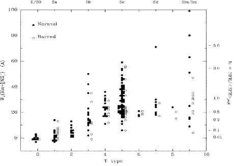
Figure 1: Distribution of integrated H + [NII] emission-line equivalent widths (a measure of star formation activity normalised to galaxy’s mass) for a large sample of nearby spiral galaxies, subdivided by Hubble type and bar morphology. The right axis scale shows corresponding values of the stellar birthrate parameter b, which is the ratio of the present SFR to that averaged over the past (from Kennicutt 1998).

The UV continuum (optimal range: 1250-2500 Å) traces directly the emissivity of a young stellar population and can be applied to star-forming galaxies over a wide range of redshifts. It is, however, very sensitive to extinction, and the relevant corrections (which may reach several magnitudes) are difficult to calibrate. This is also true for the diagnostics based on recombination lines; these lines re-emit effectively the integrated stellar luminosity of galaxies shortward of the Lyman limit; since ionizing flux is produced almost exclusively by stars with M$>$10 M_⊙, the derived SFR is very sensitive to the slope of the upper mass part of the adopted IMF. In fact, sensitivity to the IMF is a common feature of all SFR diagnostic methods. In the case of the FIR continuum (emitted by interstellar dust that has been heated by absorption of stellar light) the situation is complicated by the fact that dust may either surround young star-forming regions or be heated by the general interstellar radiation field; in the former case FIR really measures the SFR, but the situation is less clear in the latter. FIR seems then to provide an excellent measure of the SFR in dusty circumnuclear starbursts, but its application to normal disk galaxies is not straightforward.

These techniques have been used to derive the SFR in hundreds of nearby galaxies, thus revealing several interesting trends of star formation along the Hubble sequence. In Fig. 1 is plotted the equivalent width (EW) of the H$\alpha$+[NII] lines (defined as the emission line luminosity devided by the adjacent continuum flux), which is a measure of the relative SFR, i.e. the SFR normalised by unit stellar luminosity (in the red). There is a strong dispersion at each Hubble type (by a factor of $\sim$10), but also a trend of increase of the mean value, by a factor of $\sim$20 between types Sa and Sc.

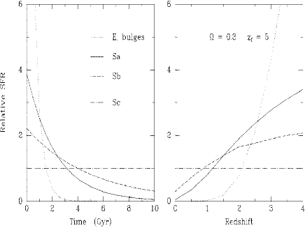
Figure 2: Schematic illustration of the evolution of the stellar birthrate for different Hubble types. The left panel shows the evolution of the relative SFR with time, following Sandage (1986). The curves for spiral galaxies are exponentially declining SFRs that fit the mean values of the birthrate parameter b measured by Kennicutt et al (1994). The curve for elliptical galaxies and bulges corresponds to an e-folding time of 0.5 Gyr, and is shown for comparative purposes only. The right panel shows the corresponding evolution in SFR with redshift, for an assumed cosmological density parameter $\Omega$= 0.3 and an assumed formation redshift z = 5 (from Kennicut 1998).

This trend should reflect the underlying past star formation histories of disks, which can be parametrised by $b$, the ratio of current SFR to the past SFR averaged over the age of the disk (i.e. Scalo 1986). Parameter $b$ (derived on the basis of population synthesis models) appears on the right axis scale of Fig. 1. Typical late type disks have formed stars at roughly constant rates ($b\sim$1) while early type spirals formed their stars quite early ($b\sim$0.01-0.1).

A schematic illustration of the corresponding star formation histories is presented in Fig. 2. On the left panel are shown the histories of typical ellipticals (and bulges of spirals) and of the disks of Sa, Sb and Sc galaxies. Obviously, in this simple picture, the Hubble sequence is uniquely determined by the caracteristic time scale of star formation.

This simple description of the Hubble sequence fails to answer two important (and probably related) questions: i) what determines the caracteristic time scales for star formation? and ii) what is the role (if any) of a galaxy’s mass in this picture? Gavazzi et al. (1996) have found an anti-correlation between the SFR per unit mass and the galaxy luminosity. Part of this trend may reflect the same dependence of SFR on Hubble type shown in Fig. 1, but it may also be that these trends are fundamentally related to the galactic mass. We shall come to this point in the next section.

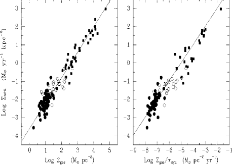
Figure 3: Left: The global Schmidt law in galaxies. Solid points denote normal spirals, squares denote circumnuclear starbursts. The open circles show the SFRs and gas densities of the central regions of the normal disks. Right: The same SFR data are plotted against the ratio of the gas density to the average orbital time in the disk (from Kennicutt 1998).

Although it is not yet clear what is the main factor affecting the SFR, it seems that on large scales there is a correlation between the SFR and the gaseous content of galaxies and starbursts. When the average SFR density $\langle\Psi\rangle$ is plotted vs. the average gas surface density $\langle\Sigma_{G}\rangle$, a Schmidt-type law is recovered: $\langle\Psi\rangle\propto\langle\Sigma_{G}\rangle^{N}$, with $N\sim$1.5 (Fig. 3 left panel). Such a law is expected if the SFR is proportional to $\rho/\tau_{FF}$ (where $\rho$ is the mass density and $\tau_{FF}\propto\rho^{-1/2}$ is the free-fall time scale) and provided the disk has a constant scale height (such as $\langle\Sigma_{G}\rangle\propto\rho$). However, Kennicut (1998) finds that the data in Fig. 3 can be equally well fit by $\langle\Psi\rangle\propto\langle\Sigma_{G}\rangle\Omega$, where $\Omega$ is the frequency of rotation of the disk measured at half the outer radius $R_{OUT}$. As noticed by Kennicutt (1998), these different parametrisations lead to different interpretations for the average efficiency $\epsilon=\langle\Psi\rangle/\langle\Sigma_{G}\rangle$ of star formation. In the former case one has $\epsilon\propto\langle\Sigma_{G}\rangle^{(N-1)}$, i.e. the efficiency is determined by the average gas surface density; in the latter case we have $\epsilon\propto\Omega$, i.e. $\epsilon$ is determined by how much mass contributes to the gravitational potential inside $R_{OUT}$/2.

These findings are extremely useful for one-zone models of galaxy evolution (treating the galaxy as a whole). However, they are of limited help for multi-zone models of disk evolution, which require prescriptions for the local SFR $\Psi(R)$, not the average one. If the local SFR is non-linear w.r.t. the gas surface density, the resulting average SFR over the whole disk will have no simple relation to the local one. Although $\langle\Psi\rangle$ can be derived from $\Psi(R)$, the inverse does not hold.

Figure 4: Upper panel: Current surface density profiles of molecular (H₂) and atomic (HI) hydrogen in the Milky Way, as a function of galactocentric radius and total gas surface density (the sum of the two, increased by 40% to account for helium). Lower panel: Corresponding theoretical current SFR (solid curve) and comparison to observational estimates of the current SFR profile. The SFR profiles are normalised to their value at $R_{S}$=8 kpc (from Boissier and Prantzos 1999).

A radial dependence of the star formation efficiency in disk galaxies is required in order to reproduce the observed abundance and colour gradients (see Sec. 4), and such a dependence has indeed been proposed on the basis of various instability criteria for gaseous disks (e.g. Talbot and Arnett 1975; Onihishi 1975; Wyse and Silk 1989; Dopita and Ryder 1994). It should be noted that star formation theories exist and may be tested mainly for disk galaxies, not for e.g. ellipticals or irregulars. A star formation rate explicitly dependent on galactocentric radius has been suggested by Onihishi (1975). It is based on the idea that stars are formed in spiral galaxies when the interstellar medium with angular frequency $\Omega(R)$ is periodically compressed by the passage of the spiral pattern, having a frequency $\Omega_{P}$=const.$<<\Omega(R)$. This leads to SFR $\propto\Omega(R)-\Omega_{P}\propto\Omega(R)$ and, for disks with flat rotation curves, to SFR $\propto$ R^-1 (Wyse and Silk 1989). In recent works (Prantzos and Silk 1998, Boissier and Prantzos 1999) we used for the Milky Way disk a local SFR of the form:

$$\Psi(R)\ =\ 0.1\ \Sigma_{G}(R)^{1.5}\ (R/R_{S})^{-1}\ {\rm M_{\odot}pc^{-2}Gyr^{-1}}$$ (1)

where $R_{S}$=8. kpc is the distance of the Sun to the Galactic centre. Such a radial dependence of the SFR is also compatible with observational evidence, as can be seen in Fig. 4, displaying the current gas surface density profile in the Milky Way disk (upper panel) and the corresponding SFR (lower pannel); comparison of this theoretical SFR to observations (lower panel in Fig. 4) shows a fairly good agreement. It has been shown that this form of the SFR can account for the observed gradients of gas fraction, SFR and chemical abundance profiles in the Milky Way (Boissier and Prantzos 1999).

3 A model for disk evolution

In our models the galactic disk is simulated as an ensemble of concentric, independently evolving rings, gradually built up by infall of primordial composition. The chemical evolution of each zone is followed by solving the appropriate set of integro-differential equations (Tinsley 1980), without the Instantaneous Recycling Approximation. Stellar yields are from Woosley and Weaver (1995) for massive stars and Renzini and Voli (1981) for intermediate mass stars. Fe producing SNIa are included, their rate being calculated with the prescription of Matteucci and Greggio (1986). The adopted stellar IMF is a multi-slope power-law between 0.1 M_⊙ and 100 M_⊙ from the work of Kroupa et al. (1993).

The spectrophotometric evolution is followed in a self-consistent way, i.e. with the SFR $\Psi(t)$ and metallicity $Z(t)$ of each zone determined by the chemical evolution, and the same IMF. The stellar lifetimes, evolutionary tracks and spectra are metallicity dependent; the first two are from the Geneva library (Schaller et al. 1992, Charbonnel et al. 1996) and the latter from Lejeune et al. (1997). Dust absorption is included according to the prescriptions of Guiderdoni et al. (1998) and assuming a “sandwich” configuration for the stars and dust layers (Calzetti et al. 1994).

3.1 Scaling relations and results

In order to extend the Milky Way model to other disk galaxies we adopt the “scaling properties” derived by Mo, Mao and White (1998, hereafter MMW98) in the framework of the Cold Dark Matter (CDM) scenario for galaxy formation. According to this scenario, primordial density fluctuations give rise to haloes of non-baryonic dark matter of mass $M$, within which baryonic gas condenses later and forms disks of maximum circular velocity $V_{C}$. It turns out that disk profiles can be expressed in terms of only two parameters: rotational velocity $V_{C}$ (measuring the mass of the halo and, by assuming a constant halo/disk mass ratio, also the mass of the disk) and spin parameter $\lambda$ (measuring the specific angular momentum of the halo). In fact, a third parameter, the redshift of galaxy formation (depending on galaxy’s mass) is playing a key role in all hierarchical models of galaxy formation. However, since the term “time of galaxy formation” is not well defined (is it the time that the first generation of stars form? or the time that some fraction of the stars, e.g. 50%, form?) we prefer to ignore it and assume that all disks start forming their stars at the same time, but not at the same rate. In that case the profile of a given disk (caracterised by the central surface density $\Sigma_{0}$ and the disk scalelength $R_{d}$) can be expressed in terms of the one of our Galaxy (the parameters of which are designated hereafter by index G):

Figure 5: Main properties of our model disks. From top to bottom: mass, central surface density and scalelength, respectively. They are plotted as a function of circular velocity $V_{C}$ and parametrised with the spin parameter $\lambda$. Disk mass depends only on $V_{C}$. Filled symbols correspond to the Milky Way model, used for the scaling of all other disks (from Boissier and Prantzos 2000).

$$\frac{R_{d}}{R_{dG}}\ =\ \frac{\lambda}{\lambda_{G}}\frac{V_{C}}{V_{CG}}\ \ \ \ {\rm and}\ \ \ \ \frac{\Sigma_{0}}{\Sigma_{0G}}\ =\left(\frac{\lambda}{\lambda_{G}}\right)^{-2}\frac{V_{C}}{V_{CG}}$$ (2)

where we have adopted $\lambda_{G}$=0.03. The absolute value of $\lambda_{G}$ is of little importance as far as it is close to the peak of he corresponding distribution function (see next paragraph), since our disk profiles and results depend only on the ratio $\lambda/\lambda_{G}$.

Eqs. 2 allow to describe the mass profile of a galactic disk in terms of the one of our Galaxy and of two parameters: $V_{C}$ and $\lambda$. The range of observed values for the former parameter is 80-360 km/s, whereas for the latter numerical simulations give values in the 0.01-0.1 range, the distribution peaking around $\lambda\sim 0.04$ (MMW98). Although it is not clear yet whether $V_{C}$ and $\lambda$ are independent quantities, we treat them here as such and construct a grid of 25 models caracterised by $V_{C}$ = 80, 150, 220, 290, 360 km/s and $\lambda$ = 0.01, 0.03, 0.05, 0.07, 0.09, respectively. [Notice: if $\lambda_{G}$=0.06 is adopted for the Milky Way, our model results would be the same, but they would correspond to values of $\lambda$ twice as large, i.e. 0.02, 0.06, 0.10, 0.14 and 0.18, respectively]. Increasing values of $V_{C}$ correspond to more massive disks and increasing values of $\lambda$ to more extended disks (Fig. 5).

Figure 6: Histories of total SFR ($\bf\Psi$, solide curve), gas mass ($\bf g$, short dashed curve) and stellar mass ($\bf s$, long dashed curve) for our disk models. Each column corresponds to a value of $\lambda$ and each row to a value of $V_{C}$. The dotted curve is an exponential fit to the SFR (from Boissier and Prantzos 2000).

We calculate the corresponding rotational velocity curves $V(R)$ of our model disks assuming contributions from the disk and an isothermal dark halo. The local SFR is then calculated self-consistently as:

$$\Psi(t,R)\ =\ \alpha\ \Sigma_{g}(t,R)^{1.5}\ V(R)\ R^{-1}$$ (3)

It can be seen that the corresponding star formation efficiency at the caracteristic radius $R_{d}$ does not depend on $V_{C}$ (for a given $\lambda$). In other terms, the adopted SFR law is important only for the resulting gradients, but not for the global properties of galaxies. In our models, the timescale for star formation is affected by the adopted infall timescale, adjusted as to form massive disks earlier than less massive ones; this most important ingredient is discussed in Sec. 3.2 and 4.

The evolution of the SFR and of the gaseous and stellar masses in our 25 disk models is shown in Fig. 6. This evolution results from the adopted prescriptions for infall and SFR. Values of SFR range from $\sim$100 $M_{\odot}$/yr in the early phases of massive disks to $\sim$0.1 $M_{\odot}$/yr for the lowest mass galaxies. The resulting SFR history is particularly interesting when compared to simple models of photometric evolution, that are usually applied in studies of galaxy evolution and of their cosmological implications. Such models (one-zone, no chemical evolution considered in general) adopt exponentially declining SFR with different caracteristic timescales for each galaxy morphological type (e.g. Bruzual & Charlot 1993, Fioc and Rocca-Volmerange 1997).

The fact that in some cases the SFR increases in time leads us to define the time-scale $\tau_{\bf*}$, required for forming the first half of the stars of a given galaxy. This time scale for star formation appears in Fig. 7, plotted as a function of $\lambda$ (left) and $V_{C}$ (right). It can be seen that $\tau_{\bf*}$ is a monotonically increasing function of $\lambda$ and a decreasing function of $V_{C}$. For the Milky Way ($V_{CG}$=220 km/s, $\lambda_{G}$=0.03) we find $\tau_{\bf*}\sim$3.5 Gyr. For galaxies less massive than the Milky Way and $\lambda>0.06$, it takes more than half the age of the Universe to form the first half of their stars.

Figure 7: Caracteristic time-scales for star formation, i.e. for forming the first half of the stars of a given galaxy, resulting from our models. They are plotted as a function of the spin parameter $\lambda$ (left) and of circular velocity $V_{C}$ (right). Filled points correspond to the Milky Way (from Boissier and Prantzos 2000).

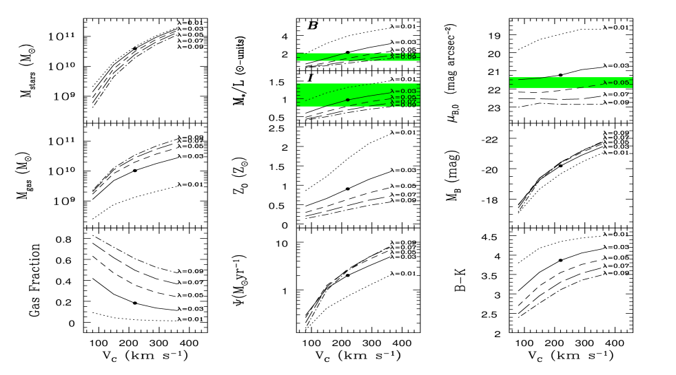
Figure 8: Integrated properties of our models at an age T=13.5 Gyr. Mass of stars (top left), mass of gas (middle left), gas fraction (bottom left), M/L values in B- and I- bands (top center), average oxygen abundance, i.e. total mass of oxygen divided by total mass of gas in the disk (middle center), star formation rate (bottom center), central surface brightness $\mu_{B0}$ (top right), total B-magnitude (middle right), total B-K (bottom right). All results are plotted as a function of the rotational velocity $V_{C}$ and parametrised with the values of the spin parameter $\lambda$. The filled symbols on the $\lambda$=0.03 curves and for $V_{C}$=220 km/s in all panels correspond to Milky Way values. The grey bands in the $M/L$ and $\mu_{B0}$ panels indicate the corresponding ranges of observed values (from Boissier and Prantzos 2000).

Assuming that all our model disks started forming their stars $\sim$13 Gyr ago, we present in Fig. 8 their integrated properties today (at redshift $z$=0). Several interesting results can be pointed out:

1) For a given $\lambda$, the stellar and gaseous masses are monotonically increasing functions of $V_{C}$. For a given $V_{C}$ disks may have considerably different gaseous and stellar contents (by factors 30 and 5, respectively), depending on how “compact” they are, i.e. on their $\lambda$ value. The more compact galaxies have always a smaller gaseous content. This is well illustrated by the behaviour of the gas fraction $\sigma_{g}$(bottom left of Fig. 8).

2) The current SFR $\Psi_{0}$ is found to be mostly a function of $V_{C}$ alone, despite the fact that the amount of gas varies by a factor of $\sim$2-3 for a given $V_{C}$. This is due to the fact that more extended disks (higher $\lambda$) are less efficient in forming stars, because of the $1/R_{d}$ factor (for a given $V_{C}$). This smaller efficiency compensates for the larger gas mass available in those galaxies, and a unique value is obtained for $\Psi_{0}$. This immediately implies that little scatter is to be expected in the B-magnitude vs. $V_{C}$ relation, and this is indeed the case as can be seen in Fig. 8 (middle right panel). For that reason we find litle scatter in the corresponding Tully-Fisher relation, which is in fair agreement with available data in various wavelength bands (as discussed in detail in Boissier and Prantzos 2000).

3) The mass to light ratio $\Upsilon=M/L$ is a quantity often used to probe the age and/or the IMF of the stellar population and the amount of dark matter, but also to convert results of dynamical models (i.e. mass) into observed quantities (i.e. light in various wavelength bands). Our models (upper middle of Fig. 8) lead to fairly acceptable values of $\Upsilon_{B}$ and $\Upsilon_{I}$; these values are confined to a relatively narrow range and a systematic (albeit weak) trend is obtained with galaxy’s mass, that should not be neglected in detailed models.

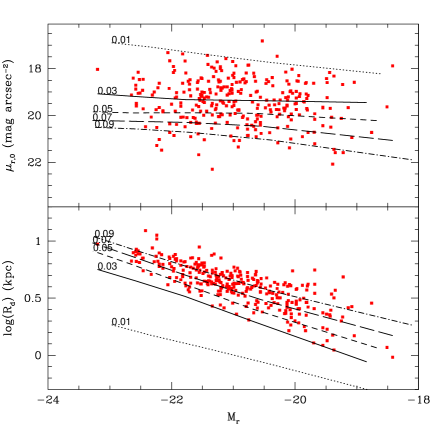
Figure 9: Central surface brightness (upper panel) and disk size $R_{d}$ (lower panel) in the r-band, as a function of the galaxy’s magnitude $M_{r}$. Our results are parametrised by the values of the spin parameter $\lambda$; $\lambda$=0.01 models produce unrealistically small disks with very high surface brightness and correspond rather to galactic bulges (from Boissier and Prantzos 2000).

4) Most of our model disks have a roughly constant current central surface brightness $\mu_{B0}\sim$21.5 mag arcsec^-2. This is quite an encouraging result, in view of the observed constancy of the central surface brightness in disks, around the “Freeman value” $\mu_{B0}$=21.7$\pm$0.3 mag arcsec^-2 (Freeman 1970); this value is indicated by the grey band in Fig. 8 (top right panel). Finally, models with $\lambda$=0.07 and 0.09 result in low surface brightness (LSB) galaxies today.

3.2 Comparison to observations

As explained in Sec. 3.1, our model disks are described by the central surface density $\Sigma_{0}$ and scalelength $R_{d}$. These are related to the “fundamental” parameters $V_{C}$ and $\lambda$ (fundamental because they refer to the dark matter haloes) through the scaling relations (2), which allow to use the Milky Way as a “calibrator”.

In Fig. 9 we present the r-band central surface brightness (upper panel) and size (lower panel) of our model disks as a function of the galaxy’s luminosity and we compare them to the data of Courteau and Rix (1999). It can be seen that:

i) The central surface brightness in our models compares fairly well to the data. For a given value of $\lambda$, $\mu_{r0}$ is quasi-independent on luminosity (or $V_{C}$), as explained in Sec. 3.1. The obtained values depend on $\lambda$, the more compact disks being brighter. All the observed values are lower than our results of $\lambda$=0.01 models. Higher $\lambda$ values bracket reasonably well the data.

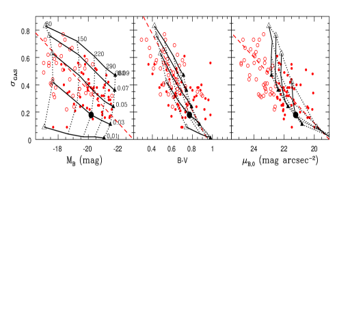
Figure 10: Gas fraction vs. B-magnitude (left panel), B-V colour (middle panel) and central surface brightness $\mu_{B0}$ (right panel). The grid of models represents 5 values for the spin parameter $\lambda$ (solid curves) and 5 values for the circular velocity (dashed curves), as indicated on the left panel. Values of $V_{C}$ run from 80 km/s (open triangle) to 360 km/s (filled triangle). Results of models are given at a galactic age of 13.5 Gyr. Data in all panels are from McGaugh and DeBlok (1997). Filled symbols correspond to high surface brightness galaxies and open symbols to low surface brightness galaxies. Our grid of models clearly does not fit the lowest surface brightness galaxies (i.e. below $\mu_{BO}$=23 mag arcsec^-2), which probably require values of $\lambda>$0.1. In all three panels, the dashed diagonal line is a fit to the data given in McGaugh and DeBlok (1997): $\sigma_{g}$ = 0.12 (M_B+23) = -1.4 [(B-V)-0.95] = 0.12 ($\mu_{BO}$-19) (from Boissier and Prantzos 2000).

ii) The size of our model disks decreases with decreasing luminosity, with a slope which matches again the observations fairly well. Our disk sizes range from $R_{d}\sim$6-10 kpc for the most luminous galaxies to 1-2 kpc for the less luminous ones. The $\lambda$=0.01 curve clearly lies too low w.r.t. all data points, showing once more that this $\lambda$ value does not produce realistic disks; it rather produces bulges or elliptical galaxies.

In Fig. 10 we compare our results to the data of McGaugh and deBlok (1997), concerning gas fraction vs. various photometric quantities. The following points can be made:

1) We find indeed a trend between gas fraction and absolute magnitude: smaller and less luminous galaxies are in general more gas rich, as can also be seen in Fig. 8 (bottom left panel). Our grid of models covers reasonnably well the range of observed values, except for the lowest luminosity galaxies (see also points 2 and 3 below). In particular, the slope of the $\sigma_{g}$ vs. M_B relation of our models is similar to the one in the fit to the data given by McGaugh and deBlok (1997).

2) We find that the observed $\sigma_{g}$ vs. B-V relation can also be explained in terms of galaxy’s mass, i.e. more massive galaxies are “redder” and have smaller gas fractions. Indeed, the slope of the $\sigma_{g}$ vs. B-V relation (-1.4) is again well reproduced by our models, and the $\lambda$=0.05 models lead to results that match close the observations. However, although our grid of models reproduces well the observed dispersion in $\sigma_{g}$, it does not cover the full range of B-V values. The lowest B-V values correspond to gas rich galaxies ($\sigma_{g}\sim$ 0.5-0.8) and could be explained by models with higher $\lambda$ values than those studies here (i.e. by very Low Surface Brightness galaxies).

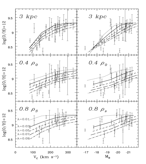
Figure 11: Oxygen abundances at various galactocentric distances: at 3 kpc (upper panels), 0.4 $\rho_{o}$ (middle panels), and 0.8 $\rho_{S}$ (lower panels). They are plotted as a function of $V_{C}$ (left) or, equivalently $M_{B}$ (right). Our results (curves) are parametrised by the corresponding $\lambda$ values.$\rho_{0}$ is the optical radius and $\rho_{S}$(=$R_{d}$ in the rest of the paper) is the disk scalelength. Data are from Zaritsky et al. (1994) (from Boissier and Prantzos 2000).

3) The situation is radically different for the $\sigma_{g}$ vs. $\mu_{B0}$ relation. As already seen in Fig. 8 (top right panel) we find no correlation in our models between $\mu_{B0}$ and $V_{C}$, but we do find one between $\mu_{B0}$ and $\lambda$: more compact disks (lower $\lambda$) have higher central surface brightness. It is this latter property that allows our models to reproduce, at least partially, the observed $\sigma_{g}$ vs. $\mu_{B0}$ relation (right panel of Fig. 10).

Another probe of the evolutionary status of a galactic disk is its metallicity. Both its absolute value and its radial profile can be used as a diagnostic tool to distinguish between different models of galactic evolution.

In Fig. 11 we plot our results at the same caracteristic radii as Zaritsky et al. (1994), i.e. at 3 kpc, at 0.4 $\rho_{0}$ and at 0.8 $R_{d}$ (from top to bottom, respectively) as a function of circular velocity $V_{C}$ (left panels) and of M_B (right panels).

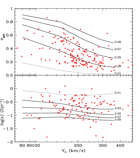
Figure 12: Upper panel : Gas fraction of spiral galaxies as a function of their circular velocity. Lower panel: Efficiency of star formation (star formation rate divided by gas mass) for those same galaxies. Model results are parametrised by teh corresponding $\lambda$ values (from Boissier et al. 2000).

It can be seen that a correlation is always found in our models between abundances ($Z$) and $V_{C}$ or M_B, stronger in the case of $Z$(3 kpc) than in the other two cases. Only in the $\lambda$=0.01 models (unrealistic for disks, as stressed already), $Z$(0.8 $R_{d}$) is not correlated with either $M_{B}$ or $V_{C}$. Except for that, the grid of our models reproduces fairly well the data, both concerning absolute values and slopes of the correlations.

3.3 Star formation efficiency

The agreement of our models to such a large body of observational data (see Boissier and Prantzos 2000 for details) is impressive, taking into account the small number of free parameters. Indeed, the only really “free” parameter is the dependence of the infall timescale on galactic mass, since all other ingredients are fixed by the calibration of the model to the Milky Way disk.

We notice that our assumption about infall timescales leads to massive disks forming their stars earlier than less massive ones. We also notice that this is not due to the corresponding star formation (SF) efficiency. As already stressed in Sec. 3.1, the efficiency of our adopted SFR is independent of $V_{C}$ (for a given $\lambda$ value). This assumption is justified by the data of Fig. 12 (lower panel). The observed current global SF efficiency of disk galaxies, measured by the ratio of the SFR to the mass of gas, seems to be independent of $V_{C}$, in fair agreement with our models (of course, higher $\lambda$ values correspond to lower efficiencies).

On the other hand, Fig. 12 (upper panel) shows also the corresponding gas fraction as a function of $V_{C}$: lower mass disks have proportionately more gas than massive ones. When the two panels of Fig. 12 are compared, there is only one possible logical conclusion: massive galaxies formed their stars earlier than their low mass counterparts.Thus, they transformed a larger fraction of their gas to stars and have today a redder stellar population and a higher metallicity at a given radius [Notice: The underlying assumption is that the SF efficiency has not varied by much during the disk history; but, if current SF efficiencies are similar for such a large range of galaxy masses and metallicities, it is difficult to see why the situation should have been very different in the past.]

These features are not easy to accomodate in the framework of currently popular hierarchical models of galaxy formation and evolution. For instance, the observed “redder” colours of more massive disks are usually interpreted in such models by invoking the presence of large amounts of dust (e.g. Somerville and Primack 1999). Although there is no doubt that the more massive the galaxy the larger is the overall amount of gas and dust (see Fig. 8), the effect should not be overestimated. Indeed, current evidence suggests that galactic disks are optically thin (e.g. Xilouris et al. 1997). Moreover, the fact that the Milky Way is “redder” than the Magellanic Clouds is certainly not due to its larger dust content….

Figure 13: Oxygen abundance gradients of our models at T=13.5 Gyr (open symbols, corresponding to the values of the spin parameter $\lambda$ as indicated in the upper panel and connected with solid curves). They are plotted as a function of the B-magnitude and compared to observations (filled symbols, with appropriate references given in each panel). Upper panel: Oxygen gradient in dex/kpc; Middle panel: Oxygen gradient in dex/R_B ($R_{B}$ is the disk scalelength in the $B$-band); Lower panel: Oxygen gradient in dex/R₂₅ ($R_{25}$ is the radius where surface brightness is 25 mag/arcsec²) (from Prantzos and Boissier 2000).

4 Abundance gradients in spirals

Almost all large spiral galaxies present sizeable radial abundance gradients. This is, for instance, the case for the Milky Way disk, showing an oxygen abundance gradient of dlog(O/H)/dR$\sim$-0.07 dex/kpc in both its gaseous and stellar components. The origin of these gradients is still a matter of debate. A radial variation of the star formation rate (SFR), or the existence of radial gas flows, or a combination of these processes, can lead to abundance gradients in disks (e.g. Henry and Worthey 1999 and references therein). On the other hand, the presence of a central bar inducing large scale mixing through radial gas flows tends to level out preexisting abundance gradients (e.g. Dutil and Roy 1999). Despite several studies in the 90ies (e.g. Friedli et al. 1998 and references therein) the relative importance of these processes has not been clarified yet.

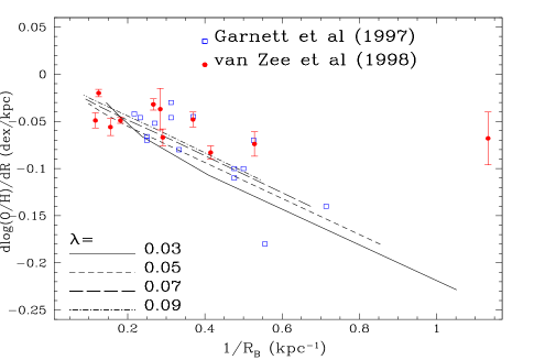
Figure 14: Predictions of our models for the gradient of metallicity (in dex/kpc) vs 1/R_B and comparison to observations. Our model results are parametrised by the corresponding values of the spin parameter $\lambda$. A clear correlation is found between abundance gradient (in dex/kpc) and 1/R_B (from Prantzos and Boissier 2000).

In Fig. 13, we compare our results to the observations of Garnett et al. (1997) and van Zee et al. (1998) concerning abundance gradients in external spirals (i.e. observations of O/H in HII regions as a function of galactocentric distance).

In the upper panel, abundance gradients are expressed in dex/kpc. Observations show that luminous disks have small gradients, while as we go to low luminosity ones the absolute value of the gradients and their dispersion increase. This trend is fairly well reproduced by our models. Indeed, the $\Sigma_{g}^{1.5}$/R factor in the adopted SFR creates large abundance variations within short distances in small galaxies. On the other hand, important gradients cannot be created in massive disks, where neighboring regions differ little in $\Sigma_{g}$.

In the middle panel of Fig. 13, the oxygen gradients are expressed in dex/R_B. When expressed in this unit, the observed abundance gradients show no more any correlation to M_B, as already noticed in Garnett et al. (1997). Moreover, a considerable dispersion is obtained for all M_B values, while the average gradient is $\sim$-0.2 dex/$R_{B}$. Since the estimates of R_B, both in observations and in our models, may be affected by extinction, we consider that the agreement of our models with the data is quite satisfactory. Another difficulty may stem from the fact that relatively few disks can be fit with perfect exponentials; according to Courteau and Rix (1999) this happens for only $\sim$20% of the disk galaxies.

In the lower panel of Fig. 13 abundance gradients are expressed in dex/R₂₅. Again, observations show no trend with M_B and a considerable dispersion. Our results also show no correlation with M_B, while the average model value ($\sim$-0.8 dex/R₂₅) is in perfect agreement with observations. This is most encouraging, since $R_{25}$ is less affected by considerations on dust extinction or fit to an exponential profile.

If one combines the conclusions of the upper and middle panel of Fig. 13, namely the facts that: a) abundance gradients (in dex/kpc) become more important and present a larger dispersion in low luminosity disks and b) abundance gradients in dex/R_B are independent of disk luminosity, then she/he immediately concludes that there must be a one-to-one correlation between abundance gradients and scalelength R_B. The correlation must be relatively tight, since the observed dispersion (middle panel of Fig. 13) is relatively small. Although this conclusion is an immediate consequence of the observations in Fig. 13, it has only been noticed recently (Prantzos and Boissier 2000).

In Fig. 14 we plot the oxygen abundance gradients (in dex/kpc) as a function of 1/R_B (which is proportional to a “magnitude gradient” in mag/kpc), both from observations and from our models. It can be seen that our models show an excellent correlation between the abundance gradients and 1/R_B: smaller disks have larger gradients and the results depend little on $\lambda$. In principle, knowing the B-band scalelength of a disk, one should be able to determine the corresponding abundance gradient and vice-versa! In practice, however, observations show a scatter around the observed trend. Since large disks “cluster” on the upper left corner of the diagram, we suggest that observations of the abundance gradients in small disks would help to establish the exact form of the correlation. The success of our models (calibrated on the Milky Way) in reproducing the observations points to a “homologuous evolution” for galactic disks, as suggested by Garnett et al. (1997) but does not explain the origin of the gradients.