Gravitational Lensing Effects on High Redshift Type II Supernova Studies with NGST

Abstract

We derive the expected Type II SN differential number counts, $N(m)$, and Hubble diagram for SCDM and LCDM cosmological models, taking into account the effects of gravitational lensing (GL) produced by the intervening cosmological mass. The mass distribution of dark matter halos (i.e. the lenses) is obtained by means of a Monte Carlo method applied to the Press-Schechter mass function. The halos are assumed to have a NFW density profile, in agreement with recent simulations of hierarchical cosmological models. Up to $z=15$, the (SCDM, LCDM) models predict a total number of (857, 3656) SNII/yr in 100 surveyed $4^{\prime}\times 4^{\prime}$ fields of the Next Generation Space Telescope. NGST will be able to reach the peak of the $N(m)$ curve, located at $AB\approx 30(31)$ for SCDM(LCDM) in $J$ and $K$ wavelength bands and detect (75%, 51%) of the above SN events. This will allow a detailed study of the early cosmic star formation history, as traced by SNIIe. $N(m)$ is only very mildly affected by the inclusion of lensing effects. In addition, GL introduces a moderate uncertainty in the determination of cosmological parameters from Hubble diagrams, when these are pushed to higher $z$. For example, for a “true” LCDM with ($\Omega_{M}=0.4,\Omega_{\Lambda}=0.6$), without proper account of GL, one would instead derive ($\Omega_{M}=0.36^{+0.15}_{-0.12},\Omega_{\Lambda}=0.60^{+0.12}_{-0.24}$). We briefly compare our results with previous similar work and discuss the limitations of the model.

1 Introduction

The star formation activity in the universe very likely started with the formation of the so-called Pop III objects (Couchman & Rees 1986, Ciardi & Ferrara 1997, Haiman et al. 1997, Tegmark et al. 1997, Ferrara 1998) at redshift $z\approx 30$. According to standard hierarchical models of structure formation, these small (total mass $M\approx 10^{6}M_{\odot}$ or baryonic mass $M_{b}\approx 10^{5}M_{\odot}$) objects merge together to form larger units. Assembling massive galaxies such as the ones observed today should take a considerable fraction of the Universe lifetime. Thus, it might be plausible that star formation at high redshift ($z\lower 2.15277pt\hbox{$\;\buildrel>\over{\sim}\;$}5$) occurred at a rate limited by the relatively small amount of baryonic fuel present in early collapsed structures. As a consequence, these objects are likely to be faint and would probably escape the detection of even the largest planned instruments.

However, unless the IMF in Pop III objects is drastically different from the local one, some of the stars formed will end their lives as supernovae (SNe). At peak luminosity, SNe could outshine their host protogalaxy by orders of magnitude and likely become the most distant observable sources since the QSO redshift distribution shows an apparent cutoff beyond $z\approx 4$ (Dunlop & Peacock 1990). Detecting high-$z$ SNe would be of primary importance to clarify the role of Pop IIIs in the reionization and reheating of the universe, and, in general, to derive the star formation history of the universe and to pose constraints on the IMF and chemical enrichment of the universe (Miralda-Escudé & Rees 1997).

The issue becomes even more interesting if we consider the gravitational lensing (GL) effects produced by the intervening cosmological mass distribution on the light emitted by SNe. The flux magnification associated with this process has been investigated in detail in a previous paper (Marri & Ferrara 1998, MF) and found to be substantially dependent on the adopted cosmological model, thus high-$z$ SNe seem to be perfect tools to constrain cosmogonies. In this paper we use the method outlined in MF but revised to include realistic lens density profiles. MF considered GL effects produced by point lenses; here we model dark halos/lenses with NFW (Navarro et al. 1997) universal density profiles derived from numerical simulations. Nonetheless, the general numerical methods and principles are the same as in MF and we refer to that paper for details; indeed this more accurate lens modeling improves the predictive power of our calculations to a level comparable to rayshooting methods based on N-body simulations, for which an extension to the high redshift studied here has not yet been possible.

We concentrate mostly on Type II SNe (SNII), although it is straightforward to extend our results to include Type I SNe (SNI). The motivation for this choice is essentially the same as in MF. SNIa are on average brighter than SNII by about 1.5 mag; moreover, SNIa are known to be very good standard candles and, for this reason, they are widely used to determine the geometry of the universe (Riess et al. 1998; Perlmutter 1998). However, it is reasonable to expect that SNI at $z\lower 2.15277pt\hbox{$\;\buildrel>\over{\sim}\;$}5$ constitute very rare events, since they arise from the explosion of C-O white dwarfs triggered by accretion from a companion; this requires evolutionary timescales comparable or larger than the Hubble time at those redshifts. A different possibility would be represented by SNIb, which originate from short-lived progenitors: however, they share problems similar to SNII, i.e. they are poorer standard candles and are fainter than SNIa.

Two different cosmological models are considered here: (i) Standard Cold Dark Matter (SCDM), with $\Omega_{M}=1,\Omega_{\Lambda}=0$, and (ii) Lambda Cold Dark Matter (LCDM): $\Omega_{M}=0.4,\Omega_{\Lambda}=0.6$. Power spectra are normalized to give the correct cluster abundance at $z=0$ ($\sigma_{8}=0.57,0.95$ for SCDM and LCDM, respectively) and we adopt the value $h=0.65$ for the adimensional Hubble constant ($H_{0}=65~{}{\rm Km}~{}{\rm sec}^{-1}{\rm Mpc}^{-1}$). We then derive high-$z$ SNII number counts expected when GL flux magnification is included for typical parameters and planned observational capabilities of the Next Generation Space Telescope (NGST, Stockman et al. 1998). The present results may serve as a guide for future mission operation mode planning.

2 Cosmic SNII Rate

To derive the cosmic rate of SNII as a function of redshift we begin by calculating the number density of dark matter halos in the two cosmologies specified above. This can be accomplished by using the Press & Schechter (1974, hereafter PS) formalism; this technique is widely used in semi-analytical models of galaxy formation (White & Frenk 1991, Kauffman 1995, Ciardi & Ferrara 1997, Baugh et al. 1998, Guiderdoni et al. 1998) and it has been shown to be in good agreement with the results from N-body numerical simulations. According to such a prescription we can write the normalized fraction of collapsed objects per unit mass at a given redshift as

$$f(M,z)=\sqrt{\frac{2}{\pi}}\frac{\delta_{c}(1+z)}{\sigma(M)^{2}}e^{-\delta_{c}^{2}(1+z)^{2}/2\sigma(M)^{2}}\left(-\frac{d\sigma(M)}{dM}\right),$$ (1)

where $\delta_{c}=1.69$ is the critical overdensity of perturbations for collapse, and $\sigma(M)$ is the gaussian variance of fluctuations on mass scale $M$. Next we calculate the star formation rate corresponding to each collapsed halo. Following Ciardi & Ferrara (1997) and Ferrara (1998) we can write the SNII rate per object of total mass $M$ as

$$\gamma(z)={\nu\Omega_{b}f_{b}\over\tau t_{ff}}M\simeq 1.2\times 10^{-7}\Omega_{b,5}f_{b,8}(1+z)_{30}^{3/2}M_{6}{\rm~{}yr}^{-1},$$ (2)

where $(1+z)_{30}=(1+z)/30$, $M_{6}=M/10^{6}M_{\odot}$. We assume a Salpeter IMF with a lower cutoff mass equal to $0.1~{}M_{\odot}$, according to which one supernova is produced for each 56 $M_{\odot}=\nu^{-1}$ of stars formed. The baryon density parameter is $\Omega_{b}=0.05\Omega_{b,5}$, of which a fraction $f_{b}\approx 0.08f_{b,8}$ (Abel et al. 1998) is able to cool and become available to form stars. The halo dark matter density is $\rho\simeq 200\rho_{c}=200[1.88\times 10^{-29}h^{2}(1+z)^{3}]$ g cm^-3; the corresponding free-fall time is $t_{ff}=(4\pi G\rho)^{-1/2}$. The star formation efficiency $\tau^{-1}=0.6\%$ is calibrated on the Milky Way.

It is well known that the star formation prescription eq. 2 would lead to a very early collapse of the baryons - with consequent star formation - in small halos, contrary to what is currently believed (Madau et al. 1996). It is therefore necessary to introduce some form of feedback, most likely due to supernova energy input into the interstellar medium of the forming galaxy. To this aim we follow the standard approach used in semi-analytical models (Kauffmann, Guiderdoni & White 1994; Baugh, Cole & Frenk 1996, Baugh et al. 1998). The star formation rate (and consequently the SN rate which is proportional to that) is weighted by the feedback function $\epsilon(M)$, whose expression is

$$\epsilon(M)={1\over 1+\epsilon_{0}\left(M_{c}/M\right)^{\alpha}}.$$ (3)

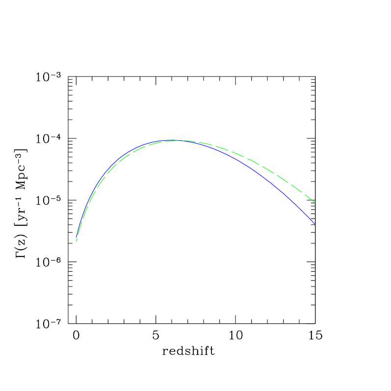
Figure 1: Comoving rate of Type II SNe as a function of redshift for the two different cosmological models: SCDM (solid line), LCDM (dashed).

The feedback function contains three free parameters: the efficiency, $\epsilon_{0}$, the critical mass for feedback, $M_{c}$, and the power, $\alpha$, which expresses the dependence of feedback on galactic mass. We choose these parameters in the following way. We first fix the value of $M_{c}=10^{10}M_{\odot}$. The motivation for this choice comes from the numerical simulations presented by MacLow & Ferrara (1999), who have shown that above that threshold galaxies lose only a negligible mass fraction of gas following moderately powerful starburst episodes. Next, we require the calculated star formation rate to best fit the observed star formation rate in the universe at redshift $\lower 2.15277pt\hbox{$\;\buildrel<\over{\sim}\;$}2$ (Lilly et al. 1996, Ellis et al. 1996). As considerable uncertainty is present on the behavior of the cosmic star formation curve at higher $z$ due to the alleged presence of extinguishing dust (Rowan-Robinson et al. 1997, Smail et al. 1997), such a choice seems to be the most conservative one. The physical interpretation of eq. 3 is that in low mass objects even a relatively small energy input is sufficient to heat (or expel) the gas, thus partially inhibiting further star formation. Although reasonable, the validity of this feedback prescription is uncertain and it should be taken, lacking a better understanding, only as a first approach to the problem. The derived comoving cosmic SNII rate, $\Gamma(z)$, is shown in Fig. 1 for the two cosmological models considered here. SCDM and LCDM models predict similar rates and at $z\lower 2.15277pt\hbox{$\;\buildrel<\over{\sim}\;$}5$, for example, our rates are broadly consistent with the SNII rates inferred using the empirical cosmic star formation history deduced from UV/optical data (Sadat et al. 1998, Madau et al. 1998).

3 Gravitational Lensing Simulations

The peak absolute magnitudes of SNII cover a wide range, overlapping SNIa at the bright end, but more generally 1.5 mag fainter. In a recent study, Patat et al. (1994) conclude that SNII seem to cluster in at least three groups, which they classify according to their B-mag at maximum as Bright ($\langle M_{B}\rangle=-18.7$), Regular ($\langle M_{B}\rangle=-16.5$), and Faint ($\langle M_{B}\rangle=-14$), respectively. Note that the Faint class is constituted by a single object, i.e. SN1987A. This classification is based on a limited sample (about 40 SNII), and therefore a statistical bias cannot be ruled out. The results of Patat et al. are also compatible with the empirical distribution law given by van den Bergh & McClure (1994) which we will use in what follows. This local SNII luminosity function (LF) is assumed not to evolve with redshift.

To obtain a statistical description of the magnification bias due to GL, we perform rayshooting simulations as described in MF. First, we fix a solid angle, $\omega_{m}=$($7.7$ arcmin)² and thus a cosmic cone in which matter is distributed among halos whose number density as a function of mass and redshift is obtained via a Monte Carlo method applied to the PS mass function. This procedure is repeated for each of the 50 slices in which the redshift range $z=1-10$ is subdivided. We study the propagation of $N_{l}=25\times 10^{6}$ light rays, uniformly covering at $z=0$ a narrower solid angle $\omega_{r}=1.5\times 10^{-6}~{}{\rm sr}$, to avoid spurious border effects. The light propagation is studied using the common multiple lens-plane approximation for a thick gravitational lens, in which the 3D matter distribution is projected onto such planes. Finally, light rays are collected within $N_{s}=1.4\times 10^{5}$ cells on each plane, thus obtaining magnification maps as a function of source position and redshift. The lower and upper limits of the lens mass distribution are equal to $10^{10}M_{\odot}$ and $10^{15}M_{\odot}$, respectively; all other parameters are the same as in MF.

The mass distribution inside a lens of total mass $M$ at a given redshift is supposed to follow the NFW (Navarro et al. 1997) density profile. The projected surface matter density, as well as the corresponding deflection angle, have been calculated by Bartelmann (1996). Using the appropriate numerical routine (kindly provided by J. Navarro), it is straightforward to calculate the relevant parameters for each lens, once the mass and redshift of the collapsed object are specified.

Differently to MF, we adopt here a full beam description of light propagation (Schneider et al. 1992) and, consequently, the average magnification is equal to unity. Such a scheme requires on each plane a negative uniform surface mass density, $\Sigma^{-}_{n}<0$, the total (negative) mass associated with this density being the one given by the sum over all lenses in the plane. As discussed in Schneider & Weiss (1988), this approach automatically guarantees flux conservation without using the Dyer-Roeder model, whose correctness is often questioned.

With this prescription for the matter distribution, the ray impact parameter as a function of discretized lens-plane redshift, $\xi_{n}$, can be recursively calculated from the following expression:

$$\xi_{n+1}=-\frac{(1+z_{n-1})D_{n,n+1}}{(1+z_{n})D_{n-1,n}}\xi_{n-1}+\frac{D_{n-1,n+1}}{D_{n-1,n}}\xi_{n}$$ (4)

$$-\frac{4G}{c^{2}}D_{n,n+1}\sum_{k=1}^{N_{n}}M^{k}_{n}F^{k}_{n}(|\xi_{n}-\xi_{n}^{k}|)\frac{\xi_{n}-\xi_{n}^{k}}{|\xi_{n}-\xi_{n}^{k}|^{2}}$$

$$-\frac{4\pi G}{c^{2}}D_{n,n+1}\Sigma^{-}_{n}\xi_{n},~{}~{}~{}~{}~{}~{}~{}~{}~{}~{}~{}$$

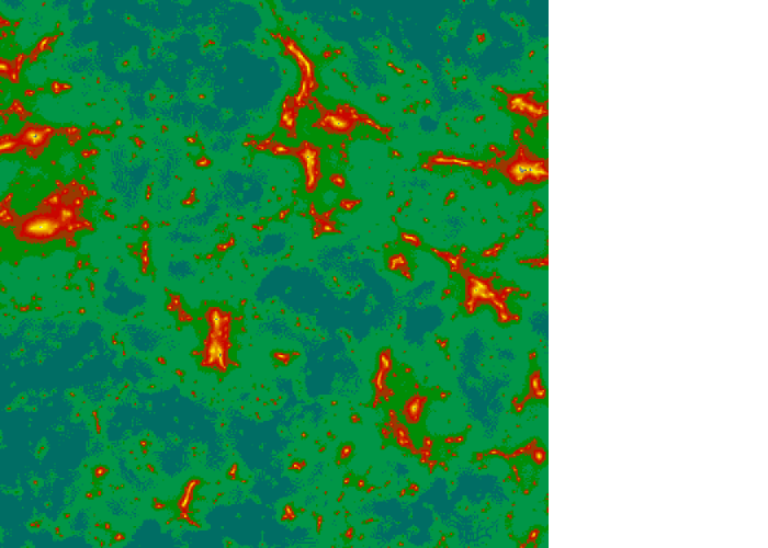
Figure 2: Magnification map for the SCDM model (4’$\times$ 4’, corresponding to a NGST field) for a source located at $z=10$. The magnification range is 0.7-50.

where symbols are as in MF, but $D(z)$ is now the usual Friedmann angular distance and the nondimensional “form factor”, $F^{k}_{n}$, depends on the model adopted for the lens density profile (provided the profile is axially-symmetric), and it is equal to unity for a point-lens; for a NFW lens the $F$-factor can be calculated using the formulae given in Bartelmann (1996). As an example, we show the resulting magnification map for the SCDM model for a source located at redshift 10 in Fig. 2.

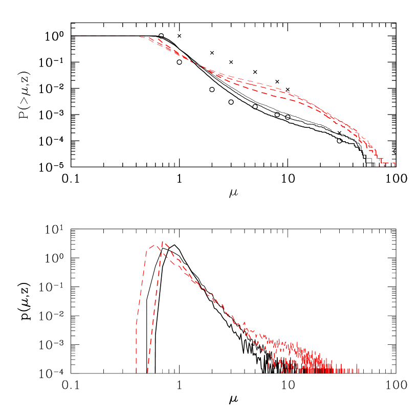
Figure 3: Top: Cumulative magnification probability. Solid curves are for SCDM, dashed curves refer to LCDM. The various curves correspond to source redshifts $z=3,5,10$ with decreasing thickness, respectively. The circles are the results of Wambsganss et al. (1998); the crosses are the results of MF (point lenses). The cosmological model in both cases is a cluster normalized, SCDM model. Bottom: Differential magnification probability. Solid curves are for SCDM, dashed curves refer to LCDM. The various curves correspond to source redshifts $z=3,5$ with decreasing thickness, respectively.

The result of the simulations relevant to the present work are the magnification probabilities at different redshifts and for the two cosmological models considered: these are shown in Fig. 3. The cumulative magnification probability, $P(>\mu)$, which expresses the probability that a source flux is magnified (or demagnified if $\mu<1$) more than $\mu$ times, is shown for $z=3,5,10$. In the lower panel the differential magnification probability is reported for the two redshifts $z=3,5$. In agreement with previous works (see e.g. Jaroszyński 1992) we find that LCDM models produce higher magnifications than SCDM models. For comparison, we plot the analogous points from the CDM GL simulation of Wambsganss et al. (1998). Also plotted for the same CDM model are the results of MF: it is clear that the assumption of point lenses in that work overpredicts the magnification with respect to the NFW density profile assumed here. We note that, as the redshift of the source is increased, larger magnifications are allowed: for example, at $z=10$ a magnification of 10 times or more has a (cumulative) probability of 0.1% in SCDM and 0.8% in LCDM models, respectively. The position of the peak of the differential magnification probability shifts toward lower $\mu$ values as $z$ increases and becomes more flatter in the vicinity of that maximum. De-magnification also becomes more pronounced, and the net effect is an increase in the flux dynamic range. Although our simulations explicitly cover the redshift range $0-10$, the behavior of $P(>\mu)$ shows that the magnification saturates well before that epoch (see also MF); we can then confidently extrapolate the curve even beyond redshift $10$. The following results are obtained assuming an upper redshift limit $z=15$, as also clear from an inspection of Fig. 1.

In order to quantify magnification effects on the observed fluxes, we need to perform the following steps: (i) calculate the total number of SNII by integrating $\Gamma(z)$ in a given redshift interval $\delta z$ around $z_{i}$ and in a certain cosmic solid angle $\omega_{obs}$; (ii) assign a peak luminosity to each SNII by randomly sampling the luminosity function; (iii) to assign an amplification to each SN we first check for multiple image events. To this aim it is necessary to identify the light rays coming from the source in the shooting plane. This is done on the fly during the simulations for a large number of cells on every plane. Once the cell is identified as the source (i.e. a SN), we reconstruct the image configuration (number of images, splitting, amplification ratios) by means of an adapted version of the friend-of-friend algorithm which isolates individual images and determines the corresponding magnifications. The very high angular resolution of NGST ($\approx 0.03$ arcsec) should be sufficient to resolve all these multiple images, whose minimum separation is typically 3 times higher (corresponding to a $M_{lens}\approx 10^{10}M_{\odot}$). Each SNe is then characterized by a redshift, an intrinsic luminosity and a GL magnification from which its observed flux can be obtained using the Friedmann luminosity distance.

As in MF, we adopt $\delta z=0.2$ and we simulate the observation of 100 NGST fields, $4^{\prime}\times 4^{\prime}$ each, i.e. $0.44$ deg², hence giving a total observed solid angle $\omega_{obs}\approx 100\times\omega_{r}$.

We suppose that these fields are surveyed for one year; in practice, one possible search startegy could be as follows. Each field is surveyed in two colors and revisited within 1 month to 1 year to find the SN candidates through their variability. The typical exposures are about $10^{3}$ s per color. After selection of good candidates, a third epoch observation in three colors, with roughly the same exposure time, is necessary to estimate the redshift and constrain the light curve. Hence, a total of about 7000 seconds per field are necessary. For about 100 fields, this observational time corresponds to a few percent of the total NGST observation time. In reality, this overestimates the allocated time for the project as the high-$z$ SN search are also a by-product of the deep galaxy and gravitational lensing surveys. A similar method, as outlined above, has been applied to the different individual frames of the HDF-N by Mannucci & Ferrara (1999) to discover a $z\approx 1$ SNIb.

The number of SNII peaks between $5\leq z\leq 10$, where about 1400 SNII occur in the cosmic volume and surveillance time considered. At even higher redshift (our computations stop at $z=15$) the total number of SNII events decreases to about 300; The two cosmological models (SCDM, LCDM) predict a total number of (857, 3656) SNII/yr in 100 NGST fields. The LCDM model offers the best perspectives for SNII detection given the higher magnification probability, and larger cosmic volume.

4 Results

The previous method allows us to build a synthetic sample of SNIIe, each of them characterized by a given luminosity, distance and gravitational amplification. This sample can be used for several cosmological applications. The most natural one consists in the prediction of the number counts of high-$z$ SNIIe as a function of wavelength bands, flux and cosmological model. Detecting these sources would enable the study of the early phases ($z\lower 2.15277pt\hbox{$\;\buildrel<\over{\sim}\;$}15$ for our specific study) of star formation in the universe, as traced by SNII. We will see in the following that the number counts are very weakly affected by the inclusion of GL effects. However, the number counts turn out to be rather sensitive to the cosmological models, mostly because of their different geometry. In addition, GL is shown below to produce considerable effects on the Hubble diagram, commonly used to constrain the geometry of the universe. We study this effect in the second part of this Section. This implies that the corresponding uncertainty in the cosmological parameter determination should be carefully treated and removed.

4.1 SNII Number Counts

In the following we compute the expected SNII number counts for our simulated sample and assess the importance of GL for such a measurement. Given the simulated SNII redshift and luminosity distribution for the two cosmological models, for each SNII we have calculated the apparent AB magnitude in four wavelength bands (JKLM), which should cover the bandpass of NGST (currently $1-5$ $\mu$m). Assuming a black-body spectrum, $B_{\nu}(T)$, at a temperature $T=25000$ K approximately $15(1+z)$ days after the explosion (Kirshner 1990, Woosley & Weaver 1986), negative $K$–corrections ($\lower 2.15277pt\hbox{$\;\buildrel<\over{\sim}\;$}-4$ for $z\lower 2.15277pt\hbox{$\;\buildrel>\over{\sim}\;$}4$) allow the detection of SNII in the above bands at high-$z$. We have taken into account absorption by IGM (Madau 1995); however, its relevance is very limited as, among the NGST bands, only the $J$ band at $z\gtrsim 9$ is weakly affected.

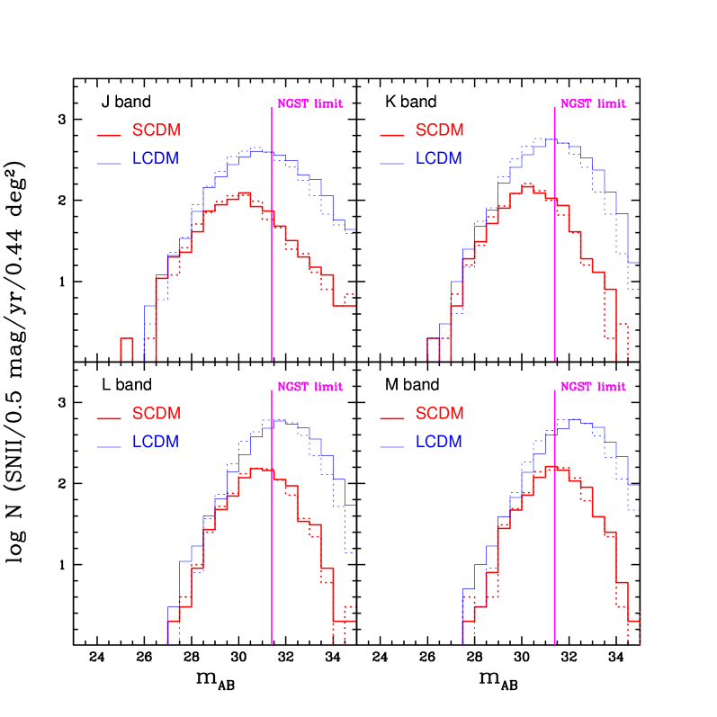
Figure 4: Differential number counts for the two cosmological models considered (thick solid line: SCDM, thin solid line: LCDM) as a function of apparent AB magnitude in $J$,$K$,$L$,$M$ bands. Also shown is the NGST limiting magnitude. Dashed curves neglect lensing magnification.

Fig. 4 shows the differential SNII counts [0.5 mag/ yr/ 0.44 deg²] as a function of AB magnitude. The four panels contain the curves for the SCDM and LCDM models and for $J$, $K$, $L$, and $M$ bands, both including or neglecting the effects of GL. For comparison, we plotted the NGST magnitude limit $AB=31.4$ (vertical line). This is calculated by assuming a constant limiting flux ${\cal F}_{NGST}=10$ nJy in the wavelength range $1-5\mu$m (i.e. $J-M$ bands). This can be achieved, for a 8-m (10-m) mirror size and a S/N=5, in about $2.6\times 10^{4}$ s ($1.1\times 10^{4}$ s). Thus, NGST should be able to reach the peak of expected SNII count distribution, which is located at $AB\approx 30-31$ for SCDM and $AB\approx 31-32$ for LCDM (depending on the wavelength band). The differences among the various bands are not particularly pronounced, although $J$ and $K$ bands present a larger number of luminous ($AB\lower 2.15277pt\hbox{$\;\buildrel<\over{\sim}\;$}27$) sources, and therefore they might be more suitable for the experiment. Furthermore, we point out that in the $L$ and $M$ bands NGST, with the current magnitude limit, will not be able to reach the peak of expected SNII count distribution in the LCDM model.

The expected number counts are only very mildly affected by the inclusion of lensing effects. As a general rule, the curves for both models become slightly broader and shifted towards fainter magnitudes by approximately 0.5 mag when gravitational lensing is taken into account. These effects are somewhat more important for the LCDM as a result of the larger magnification dynamic range in this cosmology. This behavior derives from the fact that for both models de-magnification is relatively probable, particularly at high redshift, as seen in Fig. 3.

However, a clear difference is seen in the number counts between the two models. At the NGST detection limit in the $K$-band, the (lensed) $N(m)$ ratio (SCDM:LCDM) is equal to (1:5); moreover NGST should be able to detect $\approx$ 75%(51%) of the predicted SNII by SCDM (LCDM) models in the same band. Differences between bands are similar to those outlined above.

4.2 Hubble diagram

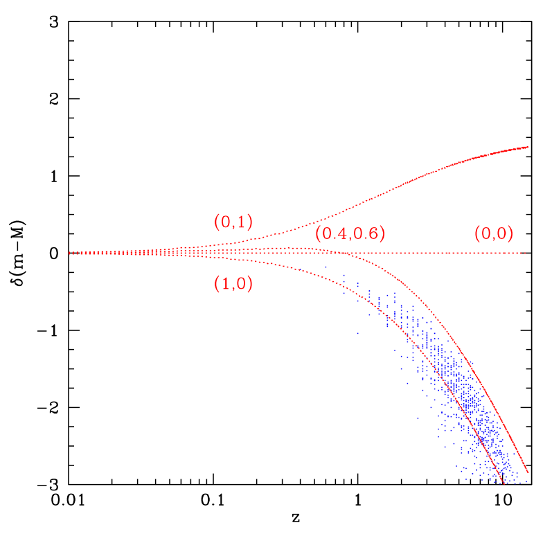
Figure 5: Hubble diagram for the simulated SNe in the SCDM model (dots). The dotted lines refer to predictions from different cosmological models without lensing effects, values of $(\Omega_{M},\Omega_{\Lambda})$ are indicated.

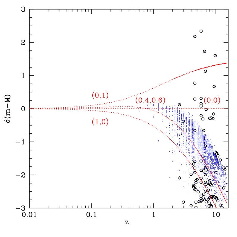
Figure 6: Same as Fig. 5 for simulated SNe in the LCDM model. Multiple images are displayed with circle dots; note that both magnified and de-magnified images are present in multiple systems.

Although the number counts are weakly affected by GL effects, the latter must be taken into account when deriving cosmological parameters from high $z$ SN experiments. To illustrate this point, we show in Figs. 5- 6 the Hubble diagrams for the SCDM and LCDM models derived from our sample. In particular, we have plotted the distance modulus difference $\delta(m-M)$ between the SNIIe in our simulated sample (shown as points), which includes GL magnification, and a specific reference model with $\Omega_{M}=0,\Omega_{\Lambda}=0$. The distance modulus for each supernova is obtained from the formula $(m-M)_{obs}=5\log[D_{lum}(z)/\sqrt{\mu(z)}]+25$, with $\mu(z)$ as derived from our GL simulations discussed above and $D_{lum}(z)$ expressed in Mpc. We assume here that the absolute magnitude $M$ can be determined within a small error. Clearly, SNIIe are not as good candles as SNIas commonly used to construct the Hubble diagram at lower redshifts. For the reasons already outlined in the Introduction, though, when exploring the more distant universe, only SNe whose progenitors were massive stars might be found, due to the small age of the universe. In addition, our understanding of the physics behind these phenomena is rapidly improving and various methods have been proposed and successfully tested in the local universe to derive the absolute magnitude of SNII once the light curve and/or their spectrum is known. These methods are reviewed in MF. Even allowing for a persisiting error in their absolute magnitudes, this spread should have a statistical nature, as opposed to the systematic one introduced by GL. Therefore, an accurate statistical analysis should be able to disentangle the two effects.

For sake of simplicity we set $h=0.65$ in the following discussion and we limit the parameter space to open and flat cosmologies with $\Omega_{k}=1-\Omega_{\Lambda}-\Omega_{M}<0.7$, $0<\Omega_{\Lambda}<1$ and $0<\Omega_{M}<1$. The luminosity distance $D_{lum}(z)$ is calculated for a Friedmann model with $\Omega_{M}$ and $\Omega_{\Lambda}$ values appropriate for the two cosmological models adopted here, i.e. SCDM and LCDM (Fig. 5 and Fig. 6, respectively). For comparison, we have also plotted the same quantity for the model $\Omega_{M}=0,\Omega_{\Lambda}=1$. The dotted curves in Figs. 5-6 are thus the distance moduli which would be observed in absence of any lensing effect in the cosmological models defined by the values of $(\Omega_{M},\Omega_{\Lambda})$ indicated above. Any source of non systematic errors (as for example the uncertainty on the SNII absolute magnitudes) would introduce a quasi-symmetric spread of the data around those curves.

The SNe in the sample (we allow for a distinction of multiple images, that are counted separately and indicated by circled dots in the Figures; note that high source magnification are associated with both amplified and deamplified multiple images) show a peculiar spread introduced by magnification/de-magnification effects. This spread is more pronounced for LCDM models, due to the flatter $P(>\mu)$ distribution obtained for this cosmology (Fig. 3). As a result, the location of the simulated data points does not lie exactly on the line corresponding to the LCDM model from which they have been derived; moreover, the points are not symmetrically distributed around it.

Stated alternatively, if the simulated points would correspond to real data, the determination of the true cosmological parameters might be affected by GL effects. In order to properly estimate the effect we let $(\Omega_{M},\Omega_{\Lambda})$ to vary and determine their best fit value by means of quadratic differences minimization of fluxes:

$$S_{F}=\sum\left[\frac{F_{i}}{L_{i}}-\frac{1}{4\pi D_{lum}^{2}}\right]^{2},$$ (5)

where $F_{i}$ and $L_{i}$ are the i-th source flux and luminosity, respectively. We neglect the intrinsic error on $L_{i}$, assuming that it could be minimized as discussed above. Once the best model is found, we look again for values of $(\Omega_{M},\Omega_{\Lambda})$ which have a quadratic deviation only $10\%$ larger than the best fit model: $S_{F}<1.1S_{F}^{min}$. Thus, for the SCDM model we find:

$$\Omega_{M}=0.97^{+0.03}_{-0.18}$$ (6)

$$\Omega_{\Lambda}=0.01^{+0.03}_{-0.01}$$

and for the LCDM model:

$$\Omega_{M}=0.36^{+0.15}_{-0.12}$$ (7)

$$\Omega_{\Lambda}=0.60^{+0.12}_{-0.24}$$

Thus, we conclude that GL has a moderate impact on the determination of cosmological parameters, the largest error being of order of 40%. As a caveat, we remark that if the same best fit method would have been instead applied directly to the modulus differences rather than on the fluxes, i.e. minimizing the quantity

$$S_{m}=\sum\left[\delta(m-M)_{i}-\delta(m-M)_{model}\right]^{2},$$ (8)

we would have deduced a much larger, albeit unphysical, discrepancy. For example, for the LCDM model we would have obtained $(\Omega_{M},\Omega_{\Lambda})\cong(0.3,0.5)$.

Although relatively small, this error due to gravitational magnification might be relevant for future experiments aiming at determining the geometry of the universe with high $z$ SNe, as if on the one hand increasing the SN distance would allow for a better discrimination among different models, on the other hand blurring of the data due to GL will jeopardize this effort, unless proper account of the effect is taken. Models such as the one presented here could be helpful to improve the fitting procedure, particularly for the most distant SNe where GL effects are stronger.

5 Comments

A great deal of both theoretical and experimental work has recently been devoted to the determination of cosmological parameters using SNIa at moderate redshifts ($z\simeq 1$). As stated above, SNII are likely to be among the most luminous (and perhaps the only visible) sources in the very distant ($z\approx 10$) universe. On the other hand, these early epochs could hold the key for the understanding of the formation of the first objects, reionization and metal enrichment of the universe. Also, the degeneracy among different cosmological models can be reduced only by extending the current studies to higher redshifts. For these reasons, it seems necessary to find ways to extract most information from these sources.

Given that techniques like the ones presented here have been applied to low redshift SNIe to assess the impact of GL, it seems instructive to briefly compare our results with those obtained in those works.

Using a numerical method based on geodetic integration, Holz (1998) calculates the magnification probability and is then able to ”correct” the SNIa Hubble diagram for the effects of GL. He argues that lensing systematically skews the apparent brightness distribution of supernovae with respect to the filled beam value of the luminosity distance. It is worth noting that he adopts two different prescriptions for the dark matter lenses: a constant distribution of halo-like objects and a compact object distribution. As was recognized also by Metcalf & Silk (1999), the two distributions yield rather different lensing probabilities. In comparison to that work, our matter distribution is self-consistently derived from CDM cosmological models. This appears to be more appropriate to study the effects arising at redshift greater than unity, where, despite the common normalization to cluster, cosmological models start to differenciate concerning their predictions on structure formation.

Wambsganss et al. (1997), use a matter distribution derived from a high resolution N-body numerical simulation of structure formation in a LCDM model. Our results agree qualitatively with theirs for what concerns the magnification probability, although we push our GL simulations up to higher redshift. In addition, we have been able to predict the number counts, via a semi-analitycal model, and therefore to build a synthetic sample enabling us to investigate the effect on an ensemble of sources rather than on a single one. As we comment in MF98 our method to reconstruct the matter distribution, given a comological model, is by large faster than using numerical simulations, allowing for an efficient inspection of the parameter space. The backdraw is that we miss the information on the spatial ditribution of lenses.

We conclude pointing out some limitations of the model which can be possibly overcome by future work. Substructure in the halos, as for example the one caused by gravitational clustering of dark matter within a single halo (Moore et al. 1999) or baryonic dissipative structures like disks in galaxy halos and, especially, galaxies in clusters, are not taken into account. A compact nature of dark matter could produce different magnification probabilities and microlensing effects. Recent results have shown that the latter effect is probably negligible, as microlensing induced variations of SN light curves can produce measurable effects only for lens masses $\lower 2.15277pt\hbox{$\;\buildrel<\over{\sim}\;$}10^{-4}M_{\odot}$ (see e.g. Kolatt & Bartelmann 1998; Porciani & Madau 1998).

We thank M. Bartelmann, L. King and P. Schneider for useful comments and discussions. Part of this work has been supported by a JILA Visitor Fellowship (AF); LP acknowledges the support of CNAA during the development of this project; SM wish to thank H. Mathis for the help in adapting the friend-of-friend algorithm.

References

- (1) Abel, T., Anninos, P., Norman, M. L. & Zhang, Y. 1998, ApJ, 508, 518
- (2) Bartelmann, M. 1996 A&A 313, 697
- (3) Baugh, C. M., Cole, S., & Frenk, C. S. 1996, MNRAS, 282L, 27
- (4) Baugh, C. M., Cole, S., Frenk, C. S., & Lacey, C. G. 1998, ApJ, 498, 504
- (5) Ciardi, B., & Ferrara, A. 1997, ApJL, 483, 5
- (6) Couchman, H. M. P. & Rees, M. J. 1986, MNRAS, 221, 53
- (7) Dunlop, J. S., Peacock, J. A. 1990, MNRAS, 247, 19
- (8) Ellis, R. S., Colless, M., Broadhurst, T., Heyl, J., & Glazebrook, K. 1996, MNRAS, 280, 235
- (9) Ferrara, A. 1998, ApJ, 499, L17
- (10) Guiderdoni, G., Hivon, E., Bouchet, F. R., & Maffei, B. 1998, MNRAS, 295, 877
- (11) Haiman, Z., Rees, M. J., & Loeb, A. 1997, ApJ, 484, 985
- (12) Holz, D. E. 1998, ApJL, 506, 1
- (13) Jaroszyński, M. 1992, MNRAS, 255, 655
- (14) Kauffmann, G. A. M., 1995, MNRAS, 274, 161
- (15) Kauffmann, G. A. M., Guiderdoni, B. & White, S. D. M. 1994, MNRAS, 267, 981
- (16) Kirshner, R. P. 1990, in ”Supernovae”, ed. A. G. Petschek, (Springer: New York), 59
- (17) Kolatt, T. S. & Bartelmann, M. 1998, MNRAS, 296, 763
- (18) Lilly, S. J., Le Fevre, O., Hammer, F., & Crampton, D. 1996, ApJ, 460, L1
- (19) MacLow, M.-M. & Ferrara, A. 1999, ApJ, 511, in press
- (20) Madau P., 1995, ApJ, 441, 18
- (21) Madau, P., Ferguson, H. C., Dickinson, M. E., Giavalisco, M., Steidel, C. C. & Fruchter, A. 1996, MNRAS, 283, 1388
- (22) Madau P., Della Valle, M. & Panagia, N. 1998, MNRAS, 279, L17
- (23) Mannucci, F. & Ferrara, A. 1999, MNRAS, 305, 55
- (24) Marri, S. & Ferrara, A. 1998, ApJ, 509, 43
- (25) Metcalf, R. B. & Silk, J. 1999, ApJL, 519, 1
- (26) Miralda-Escudé, J. & Rees, M. J. 1997, ApJ, 478, L57
- (27) Moore, B., Ghigna, S., Governato, F., Lake, G., Quinn, T., Stadel, J. & Tozzi, P. 1999, ApJL, 524, 19
- (28) Navarro, J. F., Frenk, C. S., White, S. D. M. 1997, ApJ, 490, 493
- (29) Patat, F., Barbon, R., Cappellaro, E. & Turatto, M. 1994, AA, 282, 731
- (30) Perlmutter, S. et al. 1998, Nature, 391, 51
- (31) Porciani, C. & Madau, P. 1998, astro-ph/9810403
- (32) Press, W. H. & Schechter, P. 1974, ApJ, 187, 425
- (33) Rowan-Robinson, M. et al. 1997, MNRAS, 289, 490.
- (34) Riess, A. G. et al. 1998, AJ, 116, 1009
- (35) Sadat, R., Blanchard, A., Guiderdoni, B. & Silk, J. 1998, A&A, 331, L69
- (36) Schneider, P., Ehlers, J., Falco E. E. 1992, Gravitational Lenses, Springer-Verlag, Berlin
- (37) Schneider, P. & Weiss, A. 1988, ApJ 330, 1
- (38) Smail, I., Ivison, R. J., & Blain, A. W. 1997, APJ, 490, L5
- (39) Stockman, H. S., Stiavelli, M., Im, M., & Mather, J. C. 1998, Science with the Next Generation Space Telescope, ed. E. Smith & A. Koratkar (ASP Conf. Ser.), in press
- (40) Tegmark, M., Silk, J., Rees, M.J., Blanchard, A., Abel, T. & Palla, F. 1997, ApJ, 474, 1
- (41) van der Bergh, S. & McClure, R. 1994, ApJ, 425, 205
- (42) Wambsganss, J. Cen, R. Xu, G & Ostriker, J. P. 1997, ApJL, 475, 81
- (43) Wambsganss, J., Cen, R. & Ostriker, J. P. 1998, ApJ, 494, 29
- (44) White, S. D. M. & Frenk, C. S. 1991, ApJ, 379, 52
- (45) Woosley, S. E. & Weaver, T. A. 1986, ARAA, 24, 205