Abstract

We propose a power filter $G_{p}$ for linear reconstruction of the CMB signal from one-dimensional scans of observational maps. This $G_{p}$ filter preserves the power spectrum of the CMB signal in contrast to the Wiener filter which diminishes the power spectrum of the reconstructed CMB signal. We demonstrate how peak statistics and a cluster analysis can be used to estimate the probability of the presence of a CMB signal in observational records. The efficiency of the $G_{p}$ filter is demonstrated on a toy model of an observational record consisting of a CMB signal and noise in the form of foreground point sources.

Power filtration of CMB observational data

D.I. Novikov
Astrophysics Department of Physics, Keble Road, Oxford OX1 3RH, U.K.
P. Naselsky
Rostov State University, Zorge 5, 344090 Rostov-Don, Russia
H.E. Jørgensen
Copenhagen University Observatory, Juliane Maries Vej 30, DK-2100 Copenhagen, Denmark.
P.R. Christensen
Theoretical Astrophysics Center, Juliane Maries Vej 30, DK-2100 Copenhagen, Denmark
I.D. Novikov
Theoretical Astrophysics Center, Juliane Maries Vej 30, 2100 Copenhagen, Ø Denmark
H.U. Nørgaard-Nielsen
Danish Space Research Institute, Juliane Maries Vej 30, DK-2100 Copenhagen, Denmark

1 Introduction

The exploration of anisotropy and polarization of the Cosmic Microwave Background (CMB) is fundamental in developing our knowledge about the Universe. During the last ten years several CMB measurement projects are being carried out ¹. After the successful COBE mission the attention has been focused on obtaining higher angular resolution of observational data in the range of the so-called Doppler peak and subsequent peaks. The level of the CMB anisotropy at multipoles $l>30$ up to $l\sim 10^{3}-2\cdot 10^{3}$ is a gold mine of cosmological information about the early Universe and its most important parameters. However, statistical analysis of modern observational data is extremely complicated and time consuming. This complexity leads to development of different approximate methods of the data reduction such as Wiener-filtration ^2,3, radical compression method ⁴, likelihood method, band-power method and others ^5,6,7. The existence of a large number of processing methods of observational data for different types of experiments is easily understood. Firstly, there are many difficulties and peculiarities of the measurements connected with the scan strategy, specific beam chopping, map making, etc. Secondly, the reconstruction of the parameters of the CMB signal is a sort of “inverse problem”. These difficulties are not specific for CMB measurements only. They are well known also in optical astronomy and in image reconstruction methods from satellite or airplane photography ⁸.

Which one of the data reduction methods mentioned above is the most preferable for any type of experiments? The answer of this question depends on the our “intuitive” hopes. We can use the following criterion which was suggested by Tegmark ²: “one method is better than another if it retains more of the cosmological information which operationally means that it will lead to smaller error bars on the parameter estimates”. However, before CMB image reconstruction from the observational scans is done we have no information about the structure of the signal (systematic errors, Gaussianity, different types of foreground sources and noise, etc). So, roughly speaking, the Tegmark criterion plays an important role a posteriori, when the reconstruction of the CMB by different methods is performed. We have to remember that for different strategies of observations and for different concrete experiments different methods of data processing can be considered as the most preferable. In addition different methods are preferable for different goals for using obtained data. In general, we may conclude that different methods complement each other.

The purpose of this paper is to propose and investigate a new method with the following aim: how can we estimate the probability of the presence of the CMB signal in an observational map and determine its characteristics if we have a hypothesis about its statistical properties (for example that it is Gaussian), and have a hypothesis about its power spectrum.

We suggest a new type of linear filtration of one-dimensional scans of CMB maps that is sensitive to non-Gaussian noise of any origin. This filtration does not change the primordial CMB power spectrum in contrast to the well known Wiener filter method. We use geometrical and topological characteristics such as the Minkowski functionals ^9-11 and statistics of peak distribution above and below some definite threshold ^12-15. We show, that these characteristics are very sensitive criteria of Gaussianity of the restored signal. The filtration of the two-dimensional maps of the CMB with the filter which preserves the statistical properties of the underlying signal was described in ⁷.

The full advantage of the new method can be demonstrated even on very small data sets. We apply our method to a “toy” model of a mixture of CMB signal and foreground point sources to model balloon- and ground-based measurements at the frequency band $\nu\simeq 10-200$GHz. The application of the method to real observational data will be considered in a separate paper.

The rest of this paper is organized as follows. In Section 2 we describe the model of the real experiments and describe a new so called “power filter” for reconstructing the CMB signal. Section 3 is devoted to peak statistics and cluster analysis of the CMB signal in one-dimensional records. In Section 4 we present the new reconstruction technique of the CMB spectrum from records with point sources and demonstrate the strength of our method. Section 5 contains our conclusions.

2 The model of real experiments and reconstruction of the CMB signal

The statistically isotropic distribution of the CMB temperature fluctuations on the sky is usually described by the spherical harmonics expansion $Y_{lm}(\vec{q})$:

$$T(q)=\sum_{l=1}^{\infty}\sum_{m=-l}^{l}a_{lm}B_{lm}Y_{lm}(\vec{q}),$$ (1)

where $a_{lm}$ are zero-mean Gaussian deviates, $\langle a_{lm}a^{*}_{l^{\prime}m^{\prime}}\rangle=C_{l}\delta_{ll^{\prime}}\delta_{mm^{\prime}}$, with $C_{l}$ given by the CMB power spectrum, $B_{lm}$ the antenna beam, and $\vec{q}(\theta,\varphi)$ the unit vector defining the position of the observational direction on the sky. Eq.(1) can be written for all frequency channels $\nu_{1}...\nu_{\tilde{m}}$, where $\tilde{m}$ is the number of bands. After the COBE mission, different CMB experiments such as Saskatoon, QMAP, CAT and others have observed rather small parts of the sky with higher angular resolution. They estimated statistical characteristics of the CMB signal from the maps using some specific pixelization strategy. Two future space missions, MAP and PLANCK, will cover a significantly greater part of the sky and will provide data with higher precision.

The traditional view is that most information of a Gaussian random field is contained in the multipole power spectrum $C_{l}$. As a result a great deal of efforts has gone into obtaining the best estimate of the power spectrum $C_{l}$ from the experimental data. The power spectrum $C_{l}$ describes properties of a two-dimensional map. However, there exist many balloon-borne experiments and ground-based projects which performed observations of the CMB anisotropy along one-dimensional sky patches. Besides that the future MAP and PLANCK missions will collect data from a large number of intersecting circles which will then be reconstructed into a two-dimensional sky map. Briefly speaking, because of the simplicity of data analysis in the one-dimensional case, the collection of CMB observational data in this format is an interesting option for modern anisotropy experiments.

Usually (see ref. ² for a recent review) one has a time-ordered set of data and can, knowing the adopted scan strategy, obtain a map with pixel values denoting the sum of a pure CMB signal ${\mathbf{x}}$ and different types ${\mathbf{n}}$ of noise, including foregrounds, atmospheric emission, radiometer noise and so on.

In the following we consider final maps consisting of a pure CMB signal ${\mathbf{x}}$ and noise ${\mathbf{n}}=\sum_{i}{\mathbf{n}}_{i}$ and use therefore for a one-dimensional single record

$${\mathbf{Y(t)}}={\mathbf{x}}(t)+{\mathbf{n}}(t)$$ (2)

where $t$ is an independent variable along the record.

For this simple model of the measured signal Eq.(2) one can approximately reconstruct the pure CMB signal using a linear reconstruction technique (see ⁸ for a general description of the method). Note that in Eq.(2) we do not assume the random fields ${\mathbf{x}}$ and ${\mathbf{n}}$ to be Gaussian.

The general task of linear methods of reconstruction of a signal is to obtain an approximate estimation $\overline{{\mathbf{x}}}^{\prime}(t)$ of a signal ${\mathbf{x}}(t)$ from the measured signal ${\mathbf{Y(t)}}$ using linear operations. Following ⁸ the estimation $\overline{{\mathbf{x}}}^{\prime}(t)$ of the CMB signal ${\mathbf{x}}(t)$ from Eq.(2) can be written as

$$\overline{{\mathbf{x}}}^{\prime}(t)=\int G(t-t^{\prime}){\mathbf{Y}}(t^{\prime})dt^{\prime}$$ (3)

where $G(t-t^{\prime})$ is the filter of the reconstruction.

Before describing the new method which we propose for the reconstruction of the CMB signal, let us briefly discuss the standard linear filtering methods which were reviewed by Tegmark ². Firstly, following ², we point out that linear methods of filtration of maps do not destroy information about phases which is contained in the initial maps (or one-dimensional records). Secondly, the non-linear extraction of the signal, such as band-power method ^4,5, needs some special assumptions about the statistical properties of CMB signal and noise (for example Gaussian statistics of noise). Besides that, all non-linear methods destroy information contained in the maps ².

Let us return to Eq.(2) and Eq.(3) and consider one example of CMB signal reconstruction which uses a simple Wiener filtering method ². Following ², the estimated signal from Eq.(2) is

$$\overline{{\mathbf{x}}}^{\prime\prime}(t)=\int W(t-t^{\prime}){\mathbf{Y}}(t)dt,$$ (4)

where $W(t-t^{\prime})$ is the so called Wiener filter which minimizes the reconstruction error $\Delta^{2}\equiv(\overline{{\mathbf{x}}}^{\prime\prime}-{\mathbf{x}})^{2}$. Tegmark and Efstathiou ³ and Tegmark ² have shown that the W filter has a particularly simple form in Fourier space under assumptions in Eq.(2). For this case $W$ has the following form:

$$W(k)=\frac{P_{CMB}(k)}{P_{tot}(k)}=\left(1+\frac{P_{noise}(k)}{P_{CMB}(k)}\right)^{-1},$$ (5)

where $P_{tot}(k)=P_{CMB}(k)+P_{noise}(k)$ is the power spectrum of the measured signal ${\mathbf{Y}}(t)$, $P_{CMB}(k)$ the CMB power spectrum folded with the antenna beam and $P_{noise}(k)$ the noise power spectrum.

Let us return to Eq.(4). It is straightforward to prove that the power spectrum of the reconstructed signal $P_{\overline{x}^{\prime\prime}}(k)$ is equal to

$$P_{\overline{x}^{\prime\prime}}(k)=W^{2}(k)P_{tot}(k)=P_{CMB}(k)W(k).$$ (6)

As one can see from Eq.(5), $W<1$ which, together with Eq.(6), shows that the Wiener filter decreases the CMB power spectrum of the reconstructed signal.

For a linear reconstruction of the CMB signal in one-dimensional scans we propose to use the so called “power filter” $G_{p}$ ⁸. As we told in Section 1 the corresponding consideration for two-dimensional CMB maps was done in ⁷. This filter minimizes the difference between the power spectrum $P_{\overline{x}^{\prime}}(k)$ and the CMB power spectrum. It is clear that this condition corresponds to

$$P_{\overline{x}^{\prime}}(k)=P_{CMB}.$$ (7)

We will demonstrate that for our case $G_{p}=W^{1/2}$. For the proof let us rewrite Eq.(3) for our filter $G_{p}$:

$$\overline{{\mathbf{x}}}^{\prime}(t)=\int G_{p}(t-t^{\prime}){\mathbf{Y}}(t^{\prime})dt^{\prime}.$$ (8)

Now note that from Eq.(8) one can conclude that

$$P_{x^{\prime}}(k)=G_{p}^{2}(k)P_{tot}(k).$$ (9)

Using Eq.(5), Eq.(7) and Eq.(9) we conclude that

$$G^{2}_{p}(k)=\frac{P_{CMB}(k)}{P_{tot}(k)}=W(k)$$ (10)

which proves our statement: $G_{p}=W^{1/2}$.

3 Peak statistics and cluster analysis of the reconstructed CMB signal

Using power filtration by a $G_{p}$ filter we transform the initial observational map to a reconstructed record $\{\overline{\mathbf{x}^{\prime}}(t)\}$. Like any other linear filter the $G_{p}$ filter transforms the power spectrum of the initial signal preserving phases of the signal. This property of the linear filtration is extremely important and we will consider it in more details. Let us consider a one-dimensional record $Y(t)$ and its Fourier expansion:

$$Y(t)=\sum^{\infty}_{n=1}\left[a_{n}\cos\left(\frac{2\pi nt}{\tilde{T}}\right)+b_{n}\sin\left(\frac{2\pi nt}{\tilde{T}}\right)\right],$$ (11)

where $\tilde{T}$ is the total length of a record. After a power filtration we get

$$Y^{\prime}(t)=\sum^{\infty}_{n=1}\left[a_{n}G_{n}\cos\left(\frac{2\pi nt}{\tilde{T}}\right)+b_{n}G_{n}\sin\left(\frac{2\pi nt}{\tilde{T}}\right)\right].$$ (12)

The initial power spectrum of the record (Eq.(11)) is given by

$$P_{n}^{(in)}=\frac{1}{2}(a^{2}_{n}+b^{2}_{n})$$ (13)

and of the reconstructed power spectrum (Eq.(12)) by

$$P_{n}^{(rec)}=\frac{1}{2}G^{2}_{n}(a^{2}_{n}+b^{2}_{n}).$$ (14)

However our $G_{p}$ filter does not destroy the spectrum of phases since

$$\Phi_{n}^{(in)}=\arctan\left(\frac{b_{n}}{a_{n}}\right)=\Phi_{n}^{(rec)}.$$ (15)

So, roughly speaking, we transform the power spectrum of the initial signal by $G_{p}$ filter but preserve the spectrum of phases. Thus Eq.(15) demonstrates that such a filtration preserves a Gaussian or non-Gaussian property of the modes which are not suppressed by the filter. This property is valid for all linear filters. The specific property of the $G_{p}$ filtration is that in addition to preserve the phases it also preserves the spectrum of the CMB signal. $G_{p}$ is a unique filter with this property. Cluster analysis and peak statistics ^11-14 are very sensitive to both phases and the power spectrum. Thus, if we believe that after the $G_{p}$ filtration the reconstructed signal really represents the approximate distribution of $\Delta T$ of CMB signal, it should have the same phase characteristics and the same peak statistics and properties of clusterisation which are predicted for the initial CMB signal (under an accepted hypothesis about the cosmological model). Confrontation of peak statistics and clusterisation of the reconstructed signal with the theoretical predictions is a good test of the “quality” of the reconstruction.

We will investigate how this method works in the case of one-dimensional records. In the previous section we have shown that the reconstructed record ${\mathbf{x^{\prime}}}(t)$ has the power spectrum $P_{CMB}$. We would like to point out that all non-Gaussian features of the initial signal are transformed to the reconstructed record ${\mathbf{x^{\prime}}}(t)$ because of the linear character of filtration. We also note that in the case of application of the Wiener filter, peak statistics of the reconstructed signal is different from the hypothetical CMB signal because of the change of the power spectrum.

Assuming the primordial cosmological signal to be Gaussian, we perform the test of the filtered signal with regard to Gaussianity. In fact, we calculate the probability that the filtered signal has a Gaussian nature.

The $G_{p}$ filtering obviously makes the power spectrum of the observed signal equal to the expected CMB spectrum. The rest of the information to be investigated is about the phases only. In order to perform this test, we use a geometrical approach.

We normalize the ${\mathbf{x^{\prime}}}(t)$ record to its variance: $\nu(t)\equiv\Delta T/\sqrt{\langle\Delta T^{2}\rangle}$ and consider the following characteristics of the $\nu(t)$ statistics:

A) Normalized distribution functions of maxima and minima above the threshold $\nu_{t}$:

$$f_{max}(\nu_{t})=\frac{N_{max}(\nu_{t})}{\overline{N_{max}}}\hskip 28.45274ptf_{min}(\nu_{t})=\frac{N_{min}(\nu_{t})}{\overline{N_{min}}},$$ (16)

where $N_{max}(\nu_{t})$ and $N_{min}(\nu_{t})$ are the number of maxima and minima, respectively, and $\overline{N_{max}}=N_{max}(\nu_{t}\rightarrow-\infty)$, $\overline{N_{min}}=N_{min}(\nu_{t}\rightarrow-\infty)$ are the total number of maxima and minima.

B) The global Minkowski functionals $M_{1}$ and $M_{2}$ for a one-dimensional record, which characterize the cumulative distribution function $(M_{1})$ and the Euler characteristic (genus) of the random signal $(M_{2})$. The last quantity was first introduced in cosmology by Doroshkevich ¹⁶. For the N dimensional case there are N+1 Minkowski functionals.

C) Finally we consider the mean length of the clusters above and below a constant threshold $\nu_{t}$. A one-dimensional cluster of maxima is the continuous part of the curve with $\nu(t)>\nu_{t}$ inside the interval $t\in(t_{1},t_{2})$. Here $t_{1}$ and $t_{2}$ are roots of the equation $\nu(t_{1,2})=\nu_{t}$ and $t_{2}>t_{1}$. The length $k(\nu_{t})$ of the cluster is defined as the number of peaks with height $\nu_{peak}>\nu_{t}$ in the cluster. If the value of $\nu_{t}$ is high ($\nu_{t}\gg 1$) then only high maxima (separated from each other by regions with $\nu(t)<\nu_{t}$) are present above the threshold and the typical length of a cluster is $\langle k(\nu_{t})\rangle=1$. The reduction of the threshold level $\nu_{t}$ down to $\nu_{t}\rightarrow 0$ or $\nu_{t}<0$ leads to the appearance of big clusters when maxima of smaller clusters begin to connect together and generate a new cluster. This process is characterized by the number of clusters $N_{k}(\nu_{t})$ of the length $k$ and the total number of clusters $N(\nu_{t})$ which are present in the anisotropy records for an appropriate threshold $\nu_{t}$:

$$N(\nu_{t})=\Sigma^{\infty}_{k=1}N_{k}(\nu_{t}).$$ (17)

Thus for different statistics of initial records the mean length of a cluster at threshold level $\nu_{t}$ is

$$\langle k(\nu_{t})\rangle=\frac{\Sigma^{\infty}_{k=1}kN_{k}(\nu_{t})}{\Sigma^{\infty}_{k=1}N_{k}(\nu_{t})}.$$ (18)

It is necessary to note, that only the first characteristic considered under A and the first Minkowski functional $M_{1}$ are independent. The rest of them can be represented in terms of the distribution of peaks (A). Thus, we use them only for visual clarification and representation of our results.

The defining Eq.(16) - Eq.(18) do not depend on the nature of the initial signal or its composition.

Below we use the standard definition of the spectral parameters:

$$\begin{array}[]{l}\sigma_{n}^{2}=\int k^{2n}P_{CMB}(k)dk,\hskip 85.35826ptn=0,1,2\\ \gamma=\frac{\sigma_{1}^{2}}{\sigma_{0}\sigma_{2}}\end{array}$$ (21)

where $P_{CMB}(k)$ is the one-dimensional CMB power spectrum.

The characteristics A, B and C have a rather simple form in case of a random Gaussian field ^10-12,14:

The number of maxima and minima above a threshold $\nu_{t}$ are:

$$\begin{array}[]{l}N_{max}(\nu_{t})=\frac{1}{4\pi}\frac{\sigma_{2}}{\sigma_{1}}\left(1-\Phi\left(\frac{\nu_{t}}{\sqrt{2(1-\gamma^{2})}}\right)+\gamma e^{-\frac{\nu_{t}^{2}}{2}}\left(1+\Phi\left(\frac{\gamma\nu_{t}}{\sqrt{2(1-\gamma^{2})}}\right)\right)\right)\\ N_{min}(\nu_{t})=\frac{1}{4\pi}\frac{\sigma_{2}}{\sigma_{1}}\left(1-\Phi\left(\frac{\nu_{t}}{\sqrt{2(1-\gamma^{2})}}\right)-\gamma e^{-\frac{\nu_{t}^{2}}{2}}\left(1-\Phi\left(\frac{\gamma\nu_{t}}{\sqrt{2(1-\gamma^{2})}}\right)\right)\right)\\ \overline{N_{max}}=\overline{N_{min}}=\frac{1}{2\pi}\frac{\sigma_{2}}{\sigma_{1}}\\ \end{array}$$ (25)

The Global Minkowski functionals for a one-dimensional Gaussian field are given by:

$$\begin{array}[]{l}M_{1}(\nu_{t})=\frac{1}{2}\left(1-\Phi(\frac{\nu_{t})}{\sqrt{2}})\right)\\ M_{2}(\nu_{t}))=f_{max}(\nu_{t})-f_{min}(\nu_{t})=\gamma e^{-\frac{\nu_{t}^{2}}{2}},\\ \end{array}$$ (28)

where $\Phi(x)=\frac{2}{\sqrt{\pi}}\int^{x}_{0}e^{-t^{2}}dt$.

As it has been already mentioned above, the last characteristic ($M_{2}$) can be written in terms of the peak distributions (A) ¹⁴:

$$\langle k(\nu_{t})\rangle=\frac{N_{max}(\nu_{t})}{N_{max}(\nu_{t})-N_{min}(\nu_{t})}$$ (29)

It is not difficult to demonstrate that for a Gaussian distribution all these characteristics are functions of only two variables: threshold $\nu_{t}$ and spectral parameter $\gamma$. This fact makes our analysis transparent.

To calculate the probability that the restored (filtered) signal is Gaussian, we use only the characteristic as mentioned under A. The distributions of maxima and minima, $f_{max}(\nu_{t},\gamma)$ and $f_{min}(\nu_{t},\gamma)$, above a threshold $\nu_{t}$ are monotonic functions of $\nu_{t}$ with

$$\begin{array}[]{l}f_{max}(-\infty,\gamma)=f_{min}(-\infty,\gamma)=1\\ f_{max}(+\infty,\gamma)=f_{min}(+\infty,\gamma)=0.\\ \end{array}$$ (32)

For a limited number of peaks these distributions look like a step functions with number of steps equal to the total number of maxima and minima. If the observed signal has a cosmological nature, then this function should be consistent with the smooth analytical curve (see Eq. (16) and (20)) for $\gamma$ of the CMB spectrum. In case of real observations in a limited record we deal with bad statistics (small number of peaks). For this kind of statistics we have to perform an appropriate test, e.g. a Kolmogorov-Smirnov test ¹⁷. Before applying such a test and to demonstrate the advantage of our method, we should do the following:
1. As representations of the spectrum of the filtered signal (being identical to the spectrum of the hypothetical CMB signal) we simulate a large number $n_{r}$ of different realizations of a random Gaussian field in the considered record using a FFT algorithm.
2. For each realization r=1,..,$n_{r}$ we calculate $\gamma_{r}$ using the definition (19) as well as $f^{r}_{max}$ and $f^{r}_{min}$ using Eq.(16). Furthermore we calculate the quantities:

$$\begin{array}[]{l}I_{max,real}(r,\gamma_{r})=\int_{-5}^{+5}f_{max}^{r}(\nu_{t},\gamma_{r})d\nu_{t}\\ I_{max,anal}(r,\gamma_{r})=\int_{-5}^{+5}f_{max}(\nu_{t},\gamma_{r})d\nu_{t}\\ I_{min,real}(r,\gamma_{r})=\int_{-5}^{+5}f_{min}^{r}(\nu_{t},\gamma_{r})d\nu_{t}\\ I_{min,anal}(r,\gamma_{r})=\int_{-5}^{+5}f_{min}(\nu_{t},\gamma_{r})d\nu_{t},\\ \end{array}$$ (37)

and

$$\begin{array}[]{l}\Delta_{max}=I_{max,real}-I_{max,anal}\\ \Delta_{min}=I_{min,real}-I_{min,anal},\\ \end{array}$$ (40)

where $f_{max}(\nu_{t},\gamma_{r})$, $f_{min}(\nu_{t},\gamma_{r})$ have the analytical form (20) and $f_{max}^{r}(\nu_{t},\gamma_{r})$, $f_{min}^{r}(\nu_{t},\gamma_{r})$ are distributions of maxima and minima in a given realization. In (24) we performed integrations with the limits (-5,+5) where $f_{max}$ and $f_{min}$ in practice have reached their asymptotic values given by Eq.(23). Obviously, $\gamma$ will differ slightly from one realization to another because of the cosmic variance. This difference becomes smaller for longer records. Now we derive the formal probability that the distribution of peaks corresponds to a Gaussian distribution. There are different methods to do this. One of them is the following:
3. We count the fraction of realizations, where $|\Delta_{max}(r)|$ and $|\Delta_{min}(r)|$ are greater than some positive value $z$ and calculate $P(z)$

$$\begin{array}[]{l}P_{max}(z)=\frac{N(|\Delta_{max}(r)|>z)}{n_{r}}\\ P_{min}(z)=\frac{N(|\Delta_{min}(r)|>z)}{n_{r}}\\ \end{array}$$ (43)

Here $P(z)$ represents a numerical estimate of how well the distribution of maxima and minima corresponds to a Gaussian signal.
4. For a given filtered record we can now estimate to what extent the signal has a Gaussian nature. We derive $\Delta_{max}$ and $\Delta_{min}$ to determine the probability $P(z)$. It is clear that if $P(z)$ is larger than $\approx 3$% and therefore $z$ is within the $3\sigma$ level of the distribution, there is a good chance that we observe a Gaussian signal. Alternatively one can calculate the differential functions $n(\Delta)$ of the distributions of $\Delta_{max}$ and $\Delta_{min}$ and consider the actual value $n(\Delta)$ for the filtered signal as a measure of closeness to a Gaussian signal. If this $n(\Delta)$ is greater than a few percent the filtered signal is Gaussian within the ”$3\sigma$ level” using the analogy with a standard Gaussian distribution.

One could also use a Kolmogorov-Smirnov test, some of its generalizations or other methods to be discussed in a separate paper.

In the next section we consider the application of this technique to a concrete toy model of an observed record.

4 Application of the power filtration to a toy model of an observational record

Now we demonstrate the application of the $G_{p}$ filtration and estimate to what extent we can recover the Gaussian nature of the signal. Furthermore we compare with the result from a Wiener filtration.

We consider a CMB spectrum of a standard Cold Dark Matter cosmological model with parameters: $h_{100}=0.75$, $\Omega=1$, $\Omega_{b}=0.0125$, $\Omega_{\Lambda}=0$. For this spectrum we simulate $n_{r}$ = 1000 different realizations of the random Gaussian field (using a FFT algorithm) for a record with length $360^{o}$ and with FWHM of the antenna beam equal to $0.5^{o}$. Using the definitions in the previous section we calculate the values of $\gamma_{r}$, $I_{max}$, $I_{min}$ for each realization. These values are slightly different from one record to another because of the cosmic variance. In Fig. 1 we show the dependence of $I_{max}$ and $I_{min}$ on $\gamma_{r}$ for the realizations. In the same Fig. 1 we also show the corresponding Gaussian dependences.

Now we consider one specific realization (in analogy to a realization on the sky) which is marked by a star on Fig. 1 ($\gamma$= 0.3738, $I_{max}$= 2.751 and $I_{min}$= 2.271). Next we compute for this realization $f(\nu_{t})$ (see Fig. 2a), $M_{1}(\nu_{t})$ (see Fig. 2b), rate of clusterisation ($N_{max}/(N_{max}-N_{min})$ and $N_{min}/(N_{min}-N_{max})$ as a function of $\nu_{t}$ (see Fig. 2c), and $M_{2}(\nu_{t})$ (see Fig. 2d). On Fig. 2(a-d) we also show the corresponding analytical dependence (see Eq.(25) and Eq.(28)). The graphs for the realization on Fig. 2(a-d) are only slightly different from the corresponding analytical curves given by dashed lines.

Then we add to the CMB signal a signal from 100 identical foreground point-like sources with a random distribution over the record and with an amplitude such that the rms of the maps increases by a factor $\sqrt{2}$ relative to the pure CMB signal. We consider the signal from the point-like sources as “noise”. The signal/noise ratio in this example is thus equal to 1. Of course this is not a representation of a realistic noise but only used to demonstrate the efficiency of the power filter $G_{p}$. Discussion of more realistic models will be given in a separate paper. The power spectrum of the CMB signal plus noise is computed for the same antenna beam with FWHM $0.5^{o}$. For this realization we determine $\gamma_{r}^{CMB+noise}$ and $I_{max}$ and $I_{min}$. The corresponding points are marked by crosses on Fig. 1 for the parameters $\gamma$= 0.4833, $I_{max}$= 2.871 and $I_{min}$= 2.248.

It is seen that the crosses are far away from the clouds of realizations of the CMB and far from the Gaussian points (marked by dots with the same $\gamma_{r}^{CMB+noise}$ on Fig. 1). For this realization we calculated $f_{max}$, $f_{min}$, $M_{1}$, the rate of clusterisation, and $M_{2}$ and the corresponding analytical Gaussian functions for the given $\gamma_{r}^{CMB+noise}$. The corresponding plots are presented on Fig. 3. One can see that the distributions of these values on Fig. 3(a-d) differ significantly from the corresponding Gaussian functions. This means that the CMB+noise signal is far from being Gaussian. The same is seen from Fig.1. Now we perform filtration of this CMB+noise signal using the power filter $G_{p}$. As a result we expect to obtain a reconstructed signal with the power spectrum nearly identical to the CMB power spectrum of the considered realization. The corresponding points for $I_{max}$ and $I_{min}$ are indicated in Fig. 1 by circles with the parameters $\gamma$= 0.3930, $I_{max}$= 2.782 and $I_{min}$= 2.272.

It is seen that the circles in fact are within the corresponding clouds of numerical realizations of the CMB signal and close to the corresponding Gaussian points with the same $\gamma$.

In Fig. 4 we have plotted $f_{max}$, $f_{min}$, $M_{1}$, the rate of clusterisation, and $M_{2}$ for the reconstructed signal as well as the corresponding Gaussian analytical functions. One sees that the reconstructed realization is considerably closer to Gaussianity than the CMB+noise signal, demonstrating how effective the power filter works. It is particularly important that the filtered signal has practically the same $\gamma$ as the input CMB signal. Furthermore we may get a numerical estimate of how good the power filtration really is by using the method described in Section 3. The values of $n(\Delta)$ for the filtered signal are $n(\Delta_{max})$= 0.12 and $n(\Delta_{min})$= 0.51.

For comparison we have performed a Wiener filtration of the same realization of CMB+noise signal and computed $\gamma^{W}$, $I_{max}^{W}$ and $I_{min}^{W}$. The values ($\gamma$= 0.6232, $I_{max}$= 2.930 and $I_{min}$= 2.067) are plotted as triangles on Fig. 1 together with the Gaussian values for the same $\gamma^{W}$ as dots.

One can see that the Wiener filter displaces the corresponding points far away from the clouds of realizations of the CMB signal and that the power spectrum of the reconstructed signal is very far to be spectrum of the CMB signal.

5 Conclusions

In this paper we propose to use a power filter ⁸ for linear reconstruction of the CMB signal in one-dimensional scans. The specific property of the $G_{p}$ filter is that it preserves the power spectrum of the CMB signal. Under conditions described in Section 2 we get $G_{p}=W^{1/2}$ where $W$ is the Wiener filter. Unlike the power filter $G_{p}$ the Wiener filter $W$ diminishes the power spectrum of the reconstructed signal compared to the CMB power spectrum. In section 4 we have demonstrated that peak statistics and cluster analysis can be used to estimate the efficiency of the power filtration and to estimate the probability that a CMB signal is present in an observational record. In Section 4 we also demonstrated how the power filter works using a toy model of an observational record consisting of the CMB signal and noise in the form of point like sources. We note that in the example of Section 4 we used a signal/noise ratio equal to unity as described in section 4, but tests with different toy models have demonstrated that this method works well also in the case with this ratio significantly less than unity. Discussions of more realistic models of the noise as well as application of the described method to real observations will be done in subsequent papers.

Acknowledgments
P. Naselsky and D. Novikov are grateful to the staff of TAC and the Astronomical Observatory of the Copenhagen University for providing excellent working conditions during their visit to these institutions. This investigation was supported in part by a grant ISF MEZ 300, by a grant INTAS 97-1192, by the Danish Natural Science Research Council through grant No 9701841, by Danmarks Grundforskningsfond through its support for establishment of the Theoretical Astrophysics Center, by Alexander von Humboldt-Stiftung and by the Board of the Glasstone Benefaction.

References

1. Hu., W. home page:www.sns.ias.edu/ whu/physics/physics.html

2. Tegmark., M., ApJ. Lett 480, L87, 1997.

3. Tegmark., M. and G. Efstathiou, MNRAS 281 1297, 1996.

4. Bond., J.R., A.N. Jaffe and L. Knox, Phys. Rev. D. 57 2117, 1998.

5. Knox, L., astro-ph /9902046 v 2.28 Sep. 1999.

6. Taylor., A., A. Heavens, B. Ballinger and M. Tegmark: in Proceedings of the Particle Physics and Early Universe Conference (PPPEUC), University of Cambridge, 7-11 April 1997.

7. Gorski, K.M., Proceedings of the XXXI-st Recontres de Marion Astrophysics Meeting, p.77, Editions Frontieres, (1997). astro-ph/9701191.

8. Andrews, H.C. and B.R. Hunt. Digital image restoration. New Jersey: Pentice-Hall, 1977.

9. Minkowski., H, Mathematische Annalen, 57, 443, 1903.

10. Schmalzing., J. and K. Gorski, MNRAS 297, 335, 1998.

11. Naselsky., P. and D. Novikov, ApJ., 507, 31, 1998.

12. Novikov, D., H. Feldman, S. Shandarin, Int. Journal of Modern Physics D., 8 N3, 291, 1999.

13. Naselsky., P. and D. Novikov, ApJ. Lett., 444, L1, 1996.

14. Novikov, D.I. and H.E. Jørgensen, Int. Journal of Modern Physics D., 5 N4, 319, 1996.

15. Delabrouilee, J., K. Gorski and E. Hivon, MNRAS 298, 445, 1998.

16. Doroshkevich A.G., Astrophysics 6, 320, 1970.

17. Press, W.H., S.A. Teukolsky, W.T. Vetteling and B.P. Flannery, Numerical Recipes. Cambridge University Press. 1992.

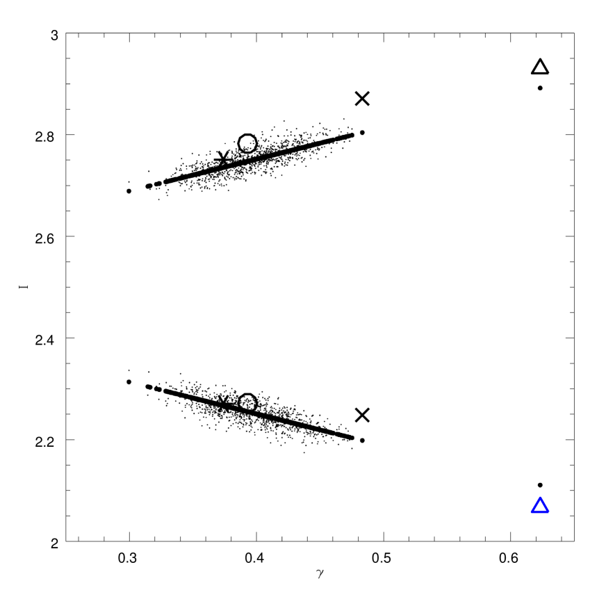
Figure 1: Dependences $I_{max}$ (upper part on vertical axis) and $I_{min}$ (lower part on vertical axis) of $\gamma$ (horizontal axis). Thick dots are dependences for Gaussian analytical expressions (20), (24). Stars correspond to the CMB realization with ($\gamma$,$I_{max}$,$I_{min}$)= (0.3738, 2.751, 2.271). Crosses correspond to the CMB+noise realization with ($\gamma$,$I_{max}$,$I_{min}$) = (0.4833, 2.871, 2.248). Circles correspond to the reconstructed signal using the $G_{p}$ filter, parameters are ($\gamma$,$I_{max}$,$I_{min}$) = (0.3930, 2.782, 2.272). Triangles correspond to the reconstructed signal with the Wiener filter; parameters are ($\gamma$,$I_{max}$,$I_{min}$) = (0.6232, 2.930, 2.067).

Figure 2: Dependences a) $f_{max}$, $f_{min}$, b) $M_{1}$, c) the rate of clusterisation $\langle k\rangle$ and d) $M_{2}$ as function of $\nu_{t}$ for a CMB realization marked on Fig. 1 by stars. Dashed lines correspond to analytical Gaussian expressions (see text). $f_{max}$ and $f_{min}$ are normalized by $\overline{N_{max}}+\overline{N_{min}}$.

Figure 3: The same as on Fig. 2 but for the CMB+noise signal (see text).

Figure 4: The same as on Fig. 2 after filtration with the $G_{p}$ filter (see text).