Chemical enrichment and star formation in the Milky Way disk

Abstract

A chromospheric age distribution of 552 late-type dwarfs is transformed into a star formation history by the application of scale height corrections, stellar evolutionary corrections and volume corrections. We show that the disk of our Galaxy has experienced enhanced episodes of star formation at 0-1 Gyr, 2-5 Gyr and 7-9 Gyr ago, although the reality of the latter burst is still uncertain. The star sample birthsites are distributed over a very large range of distances because of orbital diffusion, and so give an estimate of the global star formation rate. These results are compared with the metal-enrichment rate, given by the age–metallicity relation, with the expected epochs of close encounters between our Galaxy and the Magellanic Clouds, and with previous determinations of the star formation history. Simulations are used to examine the age-dependent smearing of the star formation history due to age uncertainties, and the broadening of the recovered features, as well as to measure the probability level that the history derived to be produced by statistical fluctuations of a constant star formation history. We show, with a significance level greater than 98%, that the Milky Way have not had a constant star formation history.

1 Introduction

The question whether the Milky Way disk has experienced a smooth and constant star formation history (hereafter SFH) or a bursty one has been the subject of a number of studies since the initial suggestions by Scalo (scalo87 (1987)) and Barry (barry (1988)). Rocha-Pinto et al. (2000a ; hereafter RPSMF) present a brief review about this question. There is evidence for three extended periods of enhanced star formation in the disk. The use of the word ‘burst’ for these features (usually lasting 1-3 Gyr) is based on the fact that all methods used to recover the SFH are likely to smear out the original data so that the star formation enhancement features could be narrower than they seem, or be composed by a succession of smaller bursts. In this sense, they were named bursts A, B and C, after Majewski (majewski (1993)).

The most efficient way to find the SFH is using the stellar age distribution, which can be transformed into a star formation history after various corrections. Twarog (twar (1980)) summarized some of these steps. Although his SFH is usually quoted as an evidence for the constancy of the star formation in the disk, he states that during the most recent 4 Gyr, the SFH has been more or less constant, followed by a sharp increase from 4 to 8 Gyr ago, and a slow decline beyond that. His unsmoothed data were also reanalysed by Noh & Scalo (noh (1990)) who have found more signs of irregularity.

Barry (barry (1988)) has improved this situation substantially by using chromospheric ages. His conclusion was criticized by Soderblom et al. (soder91 (1991)), who showed that the empirical data would be still consistent with a constant SFH if the chromospheric emission–age relation is suitably modified. However, Rocha-Pinto & Maciel (RPM98 (1998)) have recently argued that the scatter in Soderblom et al. (soder91 (1991))’s Figure 13, which is the main feature that could suggest a non-monotonic age calibration, is probably caused by contamination in the photometric indices due to the chromospheric activity. The chromospheric activity–age relation was also further investigated by Donahue (don93 (1993), don98 (1998)), and the new proposed calibration still predicts a non-constant SFH if applied to Barry’s data.

The SFH derived in this paper is based on a new chromospheric sample compiled by us (Rocha-Pinto et al. 2000b , hereafter Paper I). This paper is organized as follows: In section 2, we address the transformation of the age distribution into SFH. The results are presented in section 3. In section 4, statistical significances for the SFH are provided by means of a number of simulations. The impact of the age errors on the recovered SFH is also studied. Some comparisions with observational constraints are addressed in section 5, and each particular feature of the SFH is discussed in section 6, in view of the results from the simulations and comparisons with other data. The case for a non-monotonic chromospheric activity–age relation is discussed in section 7. Our final conclusions follow in section 8. A summary of this work was presented in RPSMF.

2 Converting age distribution into SFH

Assuming that the sample under study is representative of the galactic disk, the star formation rate can be derived from its age distribution, since the number of stars in each age bin is supposed to be correlated with the number of stars initially born at that time.

We use the same 552 stars with which we have derived the AMR (Paper I), after correcting the metallicities of the active stars for the $m_{1}$ deficiency (Giménez et al. gimenez (1991); Rocha-Pinto & Maciel RPM98 (1998)), which accounts for the influence of the chromospheric activity on the photometric indices. The reader is referred to Paper I for details concerning the sample construction and the derivation of ages, from the chromospheric Ca H and K emission measurements.

The transformation of the chromospheric age distribution into history of the star formation rate comprises three intermediate corrections, namely the volume, evolutionary and scale height corrections. They are explained in what follows.

2.1 Volume correction

Since our sample is not volume-limited, there could be a bias in the relative number of stars in each age bin: stars with different chemical compositions have different magnitudes, thus the volume of space sampled varies from star to star. To correct for this effect, before counting the number of stars in each age bin, we have weighted each star (counting initially as 1) by the same factor $d^{-3}$ used for the case of the AMR, where $d$ is the maximum distance at which the star would still have apparent magnitude lower than a limit of about 8.3 mag (see Paper I for details).

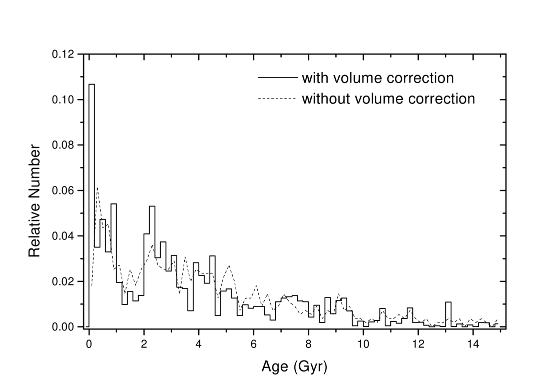
Figure 1: Chromospheric age distribution with and without volume correction, which was applied to our sample to allow the derivation of a magnitude-limited SFH.

This correction proves to change significantly the age distribution as can be seen in Figure 1.

2.2 Evolutionary corrections

A correction due to stellar evolution is needed when a sample comprises stars with different masses. The more massive stars have a life expectancy lower than the disk age, thus they would be missing in the older age bins. The mass of our stars was calculated from a characteristic mass–magnitude relation for the solar neighbourhood (Scalo scalo (1986)). In Figure 2, the mass distribution is shown. We take the mass range of our sample as 0.8 to 1.4 $M_{\odot}$, which agrees well with the spectral-type range of the sample from nearly F8 V to K1-K2 V. As an example for the necessity of these corrections, the stellar lifetime of a 1.2 $M_{\odot}$ is around 5.5 Gyr (see Figure 3 below). This means that only the most recent age bins are expected to have stars at the whole mass range of the sample.

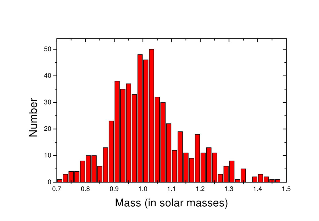
Figure 2: Mass distribution of the sample. Masses were calculated from a mean mass–magnitude relation given by Scalo (scalo (1986)). From the figure, we estimate a mass range of 0.8-1.4 $M_{\odot}$ for our sample. Note the substantial absence of massive stars, compared to the left wing of the mass distribution. The evolutionary corrections attempt to alleviate this bias.

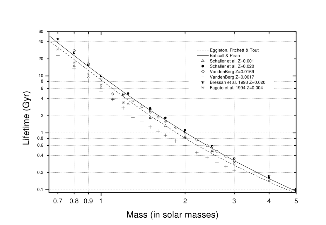
Figure 3: Stellar Lifetimes from a variety of sources: Bahcall & Piran (bahcall (1983)); VandenBerg (VandenBerg (1985)), for $Z=0.0169$ and $Z=0.0017$; Eggleton, Fitchett & Tout (EFT (1989)); Schaller et al. (schallera (1992)), for $Z=0.02$ and $Z=0.001$; Bressan et al. (bressan (1993)), for $Z=0.02$; Fagotto et al. (fagotto (1994)a), for $Z=0.004$.

The corrections are given by the following formalism. The number of stars born at time $t$ ago (present time corresponds to $t=0$), with mass between 0.8 and 1.4 $M_{\odot}$ is

$$N^{\ast}(t)=\psi(t)\int^{1.4}_{0.8}\phi(m)\,dm,$$ (1)

where $\phi(m)$ is the initial mass function, assumed constant, and $\psi(t)$ is the star formation rate in units of $M_{\odot}$ Gyr^-1pc^-2. The number of these objects that have already died today is

$$N^{\dagger}(t)=\psi(t)\int^{1.4}_{{m_{\tau}(t)}}\phi(m)\,dm,$$ (2)

where $m_{\tau}(t)$ is the mass whose lifetime corresponds to $t$. From these equations, we can write that the number of still living stars, born at time $t$, as

$$N^{\rm obs}(t)=N^{\ast}(t)-N^{\dagger}(t).$$ (3)

Using equations (1) and (2), we have

$$N^{\dagger}(t)=\left[{\int^{1.4}_{{m_{\tau}(t)}}\phi(m)\,dm\over\int^{1.4}_{0.8}\phi(m)\,dm}\right]N^{\ast}(t)={\alpha(t)\over\beta}N^{\ast}(t);$$ (4)

$$N^{\ast}(t)=\varepsilon(t)N^{\rm obs}(t),$$ (5)

where

$$\varepsilon(t)=\left(1-{\alpha(t)\over\beta}\right)^{-1}.$$ (6)

The number of objects initially born at each age bin can be calculated by using equation (6), so that we have to multiply the number of stars presently observed by the $\varepsilon$ factor. These corrections were independently developed by Tinsley (tinsley74 (1974)), in a different formalism. RPSMF present another way to express this correction in terms of the stellar lifetime probability function. We stress that all these formalisms yield identical results.

The function $m_{\tau}(t)$ can be calculated by inverting stellar lifetimes relations. Figure 3 shows stellar lifetimes for a number of studies published in the literature. Note the good agreement between the relations of the Padova group (Bressan et al. bressan (1993); Fagotto et al. fagotto (1994)a,b) and that by Schaller et al. (schallera (1992)), as well with Bahcall & Piran (bahcall (1983))’s lifetimes. The stellar lifetimes for $Z=0.0017$ given by VandenBerg (VandenBerg (1985)) are underestimated probably due to the old opacity tables used by him. The agreement in the stellar lifetimes shows that the error introduced in the SFH due to the evolutionary corrections is not very large.

The adopted turnoff-mass relation was calculated from the stellar lifetimes by Bressan et al. (bressan (1993)) and Schaller et al. (schallera (1992)), for solar metallicity stars:

$$\log m_{\tau}(t)=7.59-1.25\log t+0.05(\log t)^{2},$$ (7)

where $t$ is in yr. This equation is only valid for the mass range $5M_{\odot}>m>0.7M_{\odot}$.

We have also considered the effects of the metallicity-dependent lifetimes on the turnoff mass. To account for this dependence, we have adopted the stellar lifetimes for different chemical compositions, as given by Bressan et al. (bressan (1993)) and Fagotto et al. (fagotto (1994)a,b). Equations similar to Eq. (7) were derived for each set of isochrones and the metallicity dependence of the coefficients was calculated. We arrive at the following equation:

$$\log m_{\tau}(t)=a+b\log t+c(\log t)^{2},$$ (8)

where $a=7.62-1.56{\rm[Fe/H]}$, $b=-1.26+0.34{\rm[Fe/H]}$, $c=0.05-0.02{\rm[Fe/H]}$. Since [Fe/H] depends on time we use a third-order polynomial fitted to the AMR derived in Paper I. In that work, we have also shown that the AMR is very affected at older ages, due to the errors in the chromospheric bins. The real AMR must be probably steeper, and the disk initial metallicity around $-0.70$ dex. The effect of this in the SFH is small. The use of a steeper AMR increases the turnoff mass at older ages, decreasing the stellar evolutionary correction factors (Equation 6). As a result, the SFH features at young and intermediate age bins (ages lower than 8 Gyr) increases slightly related to the older features, in units of relative birthrate which is the kind of plot we will work in the next sections.

Note that equation (8) does not reduce to equation (7) when $\rm{[Fe/H]}=0$. The former was calculated from an average between two solar-metallicity stellar evolutionary models, while the latter uses the results of the same model with varying composition. The difference in the turnoff mass from these equations amount 12-15% from 0.4 to 15 Gyr.

The initial mass function (IMF) also enters in the formalism of the $\varepsilon$ factor. For the mass range under consideration, the IMF depends on the SFH, more specifically on the present star formation rate. It could be derived from open clusters, but they are probably severely affected by mass segregation, unresolved binaries and so on (Scalo scalo98 (1998)). We have adopted the IMF by Miller & Scalo (ms79 (1979)), for a constant SFH, which gives an average value for the mass range under study. Power-law IMFs were also used to see the effect on the results.

In Figure 4 we show how this factor varies with age. The curves represent Equations (7; dashed curve) and (8; solid curve) using the Miller-Scalo’s IMF. A third curve (shown by dots) gives the results using a Salpeter IMF with the turnoff-mass given by Equation (7). The $\varepsilon$ factor does not vary very much when we use a different IMF. Being flatter than Salpeter IMF, the correction factors given by the Miller-Scalo IMF are higher. However, the effects of neglecting the metallicity-dependence of the stellar lifetimes are much more important in the calculation of this correcting factor. Since low-metallicity stars live less than their richer counterparts, the turnoff-masses at older ages are highly affected. In the following section, we will use the $\varepsilon$ factors calculated for metallicity-dependent lifetimes.

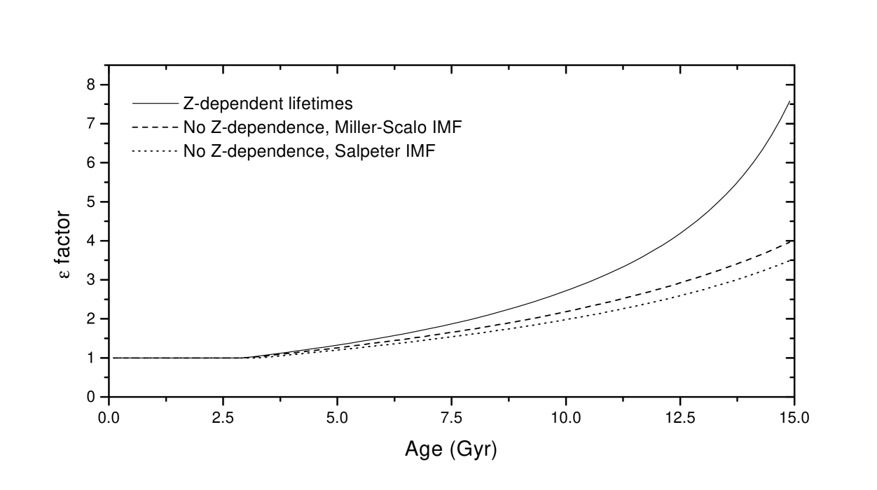
Figure 4: Stellar evolution correction factors. The curves stand for Equations (7; dashed line) and (8; solid line) and Miller-Scalo’s IMF. A third curve (dotted line) gives the results of using a Salpeter IMF with the turnoff-mass given by Equation (7).

2.3 Scale height correction

Another depopulation mechanism, affecting samples limited to the galactic plane, is the heating of the stellar orbits which increases the scale heights of the older objects. To correct for this we use the following equations. Assuming that the scale heights in the disk are exponential, the transformation of the observed age distribution, $N_{0}(t)$, into the function $N(t)$ giving the total number of stars born at time $t$ is

$$N(t)=2H(t)N_{0}(t),$$ (9)

where $H(t)$ is the average scale height as a function of the stellar age. A problem arises since scale heights are always given as a function of absolute magnitude or mass. To solve for this, we use an average stellar age corresponding to a given mass, following the iterative procedure outlined in Noh & Scalo (noh (1990)). This average age, $\langle\tau\rangle$, can be obtained by

$$\langle\tau\rangle={\int^{{\tau_{m}}}_{0}tN(t)\,dt\over\int^{{\tau_{m}}}_{0}N(t)\,dt};$$ (10)

where $\tau_{m}$ is the lifetime of stars having mass $m$, and $N(t)$ is the star formation rate. Since $\langle\tau\rangle$ depends on the star formation rate, which on the other hand depends on the average ages through the definition of $H(t)$, equations (9) and (10) can only be solved by iteration. We use the chromospheric age distribution as the first guess $N_{0}(t)$, and calculate the average ages $\langle\tau\rangle_{0}$. These are used to convert $H(m)$ to $H(t)$, and the star formation history is found by equation (9), giving $N_{1}(t)$. This quantity is used to calculate $\langle\tau\rangle_{1}$ and a new star formation rate, $N_{2}(t)$. Note that, in equation (9), the quantity that varies in each iteration is $H(t)$, not the chromospheric age distribution $N_{0}(t)$. Our calculations have shown that convergence is attained rapidly, generally after the second iteration.

Great uncertainties are still present in the scale heights for disk stars. Few works have addressed them since Scalo (scalo (1986))’s review (see e.g., Haywood, Robin & Crezé hay (1997)). We will be working with two different scale heights: Scalo (scalo (1986)) and Holmberg & Flynn (holmberg (2000)), that are shown in Figure 5. Haywood et al.’s scale heights are just in the middle of these, so they set the limits on the effects in the derivation of the SFH.

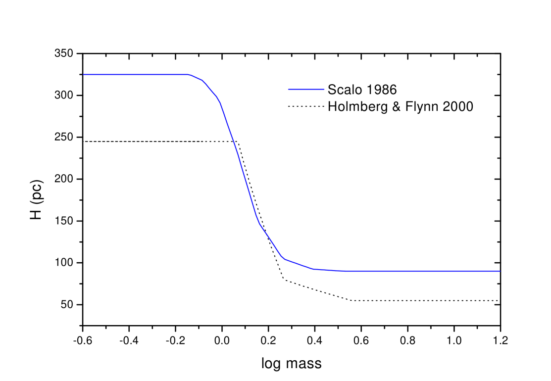
Figure 5: Scale heights given by Scalo (scalo (1986), solid line) and Holmberg & Flynn (holmberg (2000), dotted line).

The major effect of the scale heights is to increase the contribution of the older stars in the SFH. Better scale heights would not change significantly the results, so that we limit our discussion to these two derivations.

3 Star formation history in the galactic disk

3.1 Previous chromospheric SFH determinations

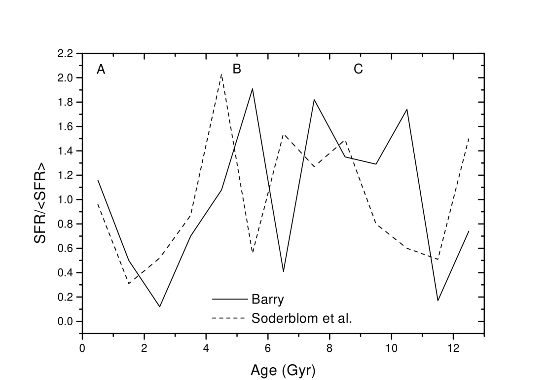
Figure 6: Comparison between chromospheric SFHs published in the literature: Barry (barry (1988), according to Noh & Scalo noh (1990)) and Soderblom et al. (soder91 (1991), according to Rana & Basu ranabasu (1992)). The position of bursts A, B and C (named after Majewski majewski (1993)) are marked.

In Figure 6, we show a comparison between two SFHs, derived from chromospheric age distributions available in the literature: Barry (barry (1988), SFH given by Noh & Scalo noh (1990)) and Soderblom et al. (soder91 (1991), SFH given by Rana & Basu ranabasu (1992)). In this plot, as well as in subsequent figures, the SFH will be expressed always as a relative birthrate, which is defined as the star formation rate in units of average past star formation rate (see Miller & Scalo ms79 (1979), for rigorous definition).

Note that the SFHs in Figure 6 are very similar to each other, a result not really surprising since Soderblom et al. have used the same sample used by Barry. On the other hand, the corresponding events in Barry’s SFH appears 1 Gyr earlier in Soderblom et al.’s SFH. The different age calibrations used in these works are the sole cause of this discrepancy. Barry makes use of Barry et al. (barry87 (1987))’s calibration which used a low-resolution index analogous to Mount Wilson $\log R^{\prime}_{\rm HK}$, while Soderblom et al. use a calibration derived by themselves. In Figure 7, we show a comparison of the ages for Barry (barry (1988))’s stars using both age calibrations. The difference in the ages are clearly caused by the slopes of the calibrations. Barry et al. (barry87 (1987))’s calibration gives higher ages compared to the other calibration, which explains the differences in the corresponding SFHs published.

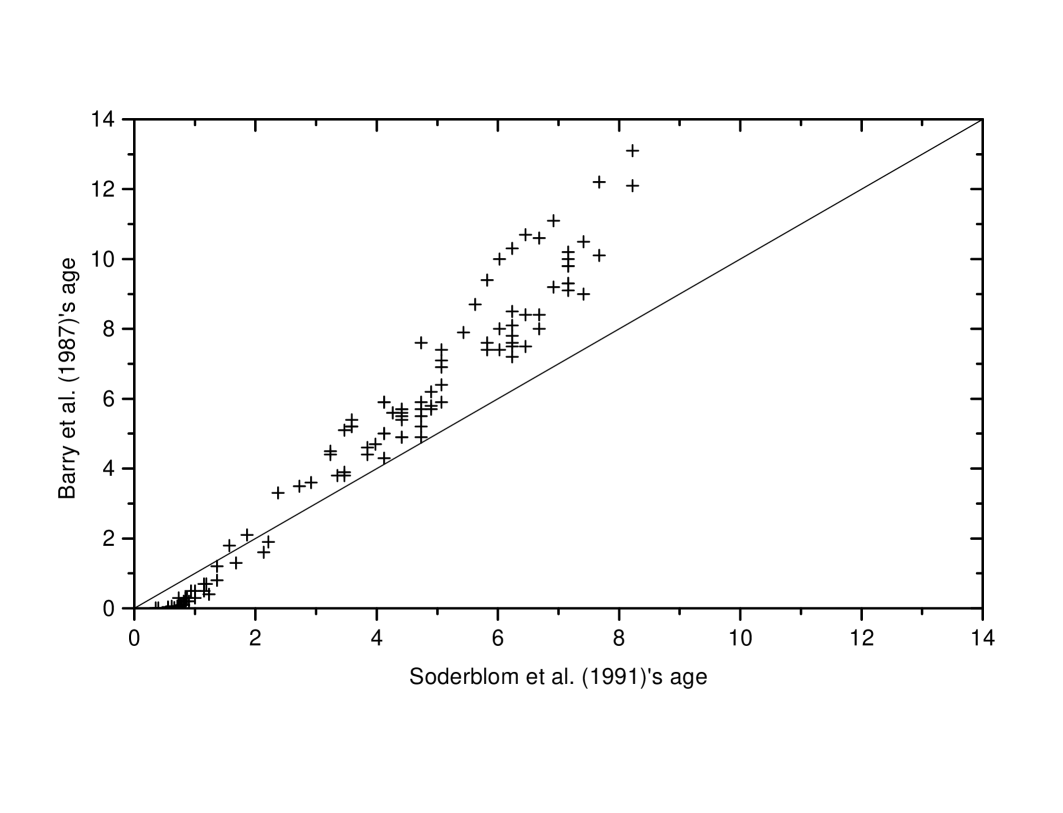
Figure 7: Comparison of stellar ages (in Gyr) in the calibrations by Barry et al. (barry87 (1987))’s and Soderblom et al. (soder91 (1991)). The first age calibration seems to overestimate the chromospheric ages by around 1 Gyr.

3.2 Determination of the SFH

The three corrections described in section 2 are applied to our data in the following order: the age distribution is first weighted according to the volume corrections, then each age bin is multiplied by the $\varepsilon$ factor and we iterate the result according to equations (9) and (10). The final result is the best estimate of the star formation history. It is shown in Figure 8a, for an age bin of 0.4 Gyr and Scalo’s scale height. There can be seen three regions where the stars are more concentrated: at 0-1 Gyr, 2-5 Gyr and 7-9 Gyr ago. Beyond 10 Gyr of age, the SFH is very irregular, probably reflecting more the sample incompleteness in this age range, and age errors, than real features. These patterns are still present even considering a smaller age bin of 0.2 Gyr. Figure 8b shows the same for Holmberg & Flynn (holmberg (2000)) scale heights. The only difference comes from the amplitude of the events. In this plot, the importance of the older bursts is increased, since in Holmberg & Flynn (holmberg (2000)) the difference in the scale heights of the oldest to the youngest stars is greater than the corresponding value in Scalo’s scale heights.

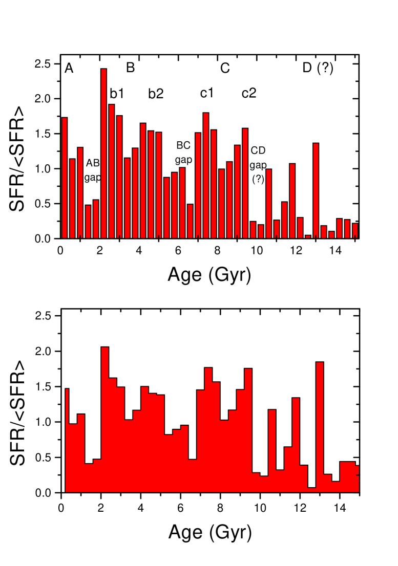
Figure 8: Star formation rate for an age bin of 0.4 Gyr. The nomenclature used by Majewski (majewski (1993)) was extended to be used with the main features of the SFH. The terms B1 and B2, and C1 and C2, stand for substructures of the supposed bursts B and C, respectively. Also shown is the supposed burst D. The gaps between the peaks are named AB gap, BC gap, and so on. The upper and lower panels show the SFH using Scalo (scalo (1986)) and Holmberg & Flynn (holmberg (2000)) scale heights, respectively.

We have used an extended nomenclature to that of Majewsky (majewski (1993)) to refer to the features found. At the age range where bursts B and C were thought to occur double-peaked structures are now seen. Thus, we have used the terms B1 and B2, and C1 and C2, to these substructures. Also shown is the supposed burst D, as Majewski (majewski (1993)) had suggested. Their meaning will be discussed later. The lulls between the bursts were named AB gap, BC gap and so on. Some of us have previously referred to the most recent lull as ‘Vaughan-Preston gap’. We now avoid the use of this term because:

1. The Vaughan-Preston gap is a feature in the chromospheric activity distribution;

2. Due to the metallicity-dependence of the age calibration, the Vaughan-Preston gap is not linearly reflected in an age gap;

3. Henry et al. (HSDB (1996), hereafter HSDB) shows that the Vaughan-Preston gap is less pronounced than was earlier thought, and does not resemble a gap but a transition zone.

Comparing with other studies in the literature, the SFH seems particularly different. There are still three major star formation episodes but their amplitude, extension and time of occurrence are not identical to those that were previously found by other authors. Table 1 summarizes the main characteristics of our SFH comparing to that of Barry (barry (1988), as derived in Noh & Scalo noh (1990)). In the Table, the entries with two values stand for the SFH derived with different scale heights. The first number refers to the SFH with Scalo’s scale height, and the other refers to that with Holmberg & Flynn’s.

Table 1: Main features of the SFH compared with Barry (barry (1988)).

	This work	Barry (barry (1988))
Number of ‘bursts’	3	3
Age of burst A	0-1 Gyr	0-1 Gyr
Age of burst B	2-5 Gyr	4-6 Gyr
Age of burst C	7-9.5 Gyr	7-11 Gyr
Stronger burst	B	B
Duration of the most recent lull (AB gap)	1 Gyr	$\leq$ 3 Gyr
(% of stars formed in burst A)/Gyr	10.48/9.58	8.92
(% of stars formed in burst B)/Gyr	10.40/9.72	11.50
(% of stars formed in burst C)/Gyr	8.88/10.88	11.92

As we can see, the main events of our SFH seem to occur earlier than the corresponding events in Barry’s SFH, by approximately 1 Gyr. This can also be seen in Figure 6: the SFR from Soderblom et al. (soder91 (1991))’s data have features earlier than Barry by about 1 Gyr. This comes mainly from the use of Soderblom et al. (soder91 (1991))’s age calibration on which we have based our ages. This hypothesis is reinforced by the fact that the fraction of the stars formed in each burst is in reasonable agreement with the corresponding events in Barry’s SFH (see Table 1). The events we have found are most likely to be the same that have appeared in previous works, and the difference in the time of occurrence comes from the shrinking of the chronologic scale of the age calibration.

The narrowing of the AB gap is one of the main differences of our SFH and that found by Barry. This can be expected since our sample does not show a well-marked Vaughan-Preston gap, contrary to what is found in the survey of Soderblom (soder (1985)), from which Barry (barry (1988)) selected his sample.

Some other differences in the amplitude and duration of the bursts can be understood as resulting from the differences in the samples used by us and by Barry. Nearly 70% of our stars come from HSDB survey. We have already shown in Paper I that HSDB and Soderblom (soder (1985)) surveys have different chromospheric activity distributions. These are directly reflected in the SFH.

We have found double peaks at bursts B and C. At the present moment we cannot distinguish these features from a real double-peaked burst (that is, two unresolved bursts) or a single smeared peak. However, it is interesting to see that the previous chromospheric SFHs give some evidence for a double burst C. In Figure 6 burst C also seems to be formed by two peaks. On the other hand, the same does not occur for burst B. The feature called B2 corresponds more closely to burst B in the previous studies, but at the age where we have found B1, the other SFHs show a gap.

The resulting SFH comes directly from the age distribution, in an approach which assumes that the most frequent ages of the stars indicate the epochs when the star formation was more intense. Both the evolutionary and the scale height corrections do not change the clumps of stars already present in the age distribution. The only correction which could introduce spurious patterns in it is the volume correction, which must be applied before the other two. Figure 1 shows how it affects the age distribution. It is elucidating that the major patterns of the age distributions are not much changed after this correction. We refer basically to the clumps of stars younger than 1 Gyr and stars with ages between 2 and 4 Gyr. These clumps will be identified with burst A and B, respectively, after the application of the other corrections. Note also, that the AB gap is clearly seen in the age distribution before the volume correction. In spite of it, it is necessary to know if the presence of stars with very high weights (due to their proximity and low temperature) could affect the results. Therefore, we have recalculated the SFH now disregarding the stars that have very high weights after the volume correction. We have cut the sample to those stars with weights not exceeding 2$\sigma$ and 3$\sigma$. The resulting SFHs is compared to the SFH of the whole sample in Figure 9. It is possible to see that the presence of outliers does not affect the global result. The uncertainty introduced affects mainly the amplitude of the events, at a level similar to that introduced by the uncertainty in the scale heights. We believe that the volume correction has not impinged artificial patterns on the data, and that the star formation just derived reflects directly the observed distribution of stellar ages in the solar vicinity.

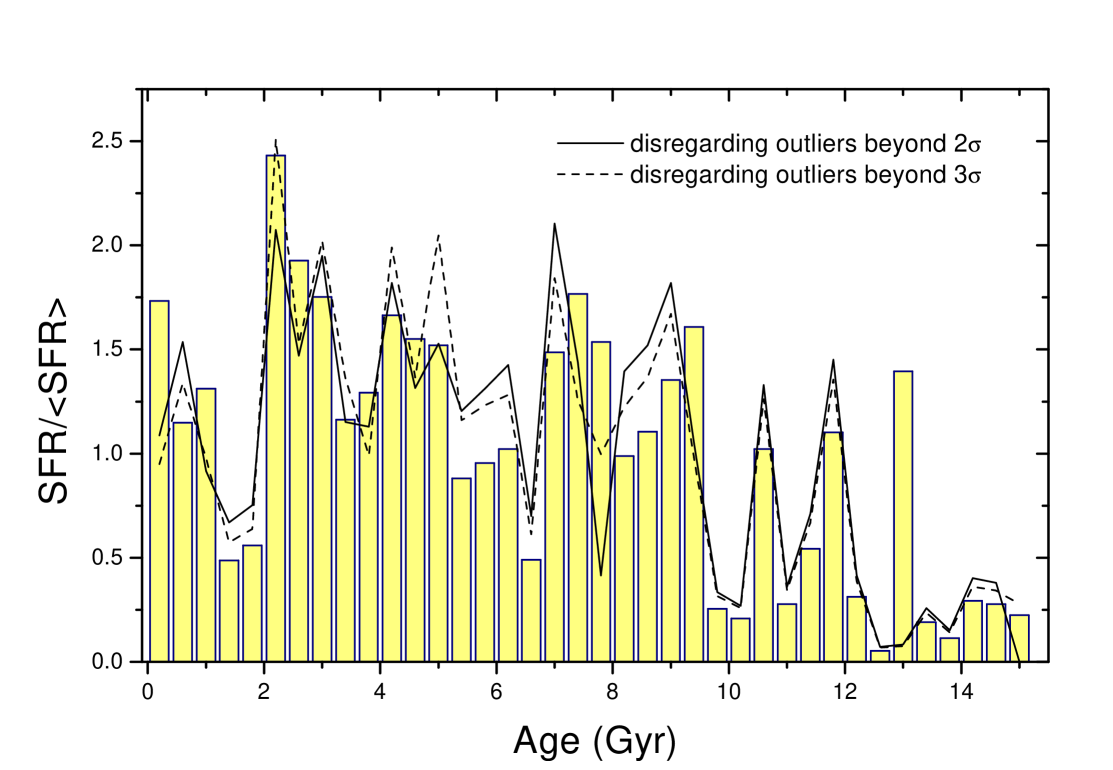
Figure 9: Star formation rate calculated after disregarding outliers with weights exceeding 2$\sigma$ (solid line) and 3$\sigma$ (dashed line), after the volume corrections, compared to the history used throughout this paper.

4 Statistical significance of the results

4.1 Inconsistency of the data with a constant SFH

There is a widespread myth on galactic evolutionary studies about the near constancy of the SFH in the disk. This comes primarily from earlier studies setting constraints to the present relative birthrate (e.g., Miller & Scalo ms79 (1979); Scalo scalo (1986)). The observational constraints have favoured a value near unity, and that was interpreted as a constant SFH.

This constraint refers only to the present star formation rate. As pointed out by O’Connell (oconnell (1997)) and Rocha-Pinto & Maciel (RPM97 (1997)), it is not the same as the star formation history.

A typical criticism to a plot like that shown in Figure 8 is that the results still do not rule out a constant SFH, since the oscilations of peaks and lulls around the unity can be understood as fluctuations of a SFH that was ‘constant’ in the mean. This is an usual mistake of those who are accustomed to the strong, short-lived bursts in other galaxies.

The ability to find bursts of star formation depends on the resolution. Suppose a galaxy that has experienced only once a real strong star formating burst during its entire lifetime. The burst had an intensity of hundred times the average star formation in this galaxy, and has lasted $10^{7}$ yr, which are typical parameters of bursts in active galaxies. Figure 10 shows how this burst would be noticed, in a plot similar to that we use, as a function of the bin size. In a bin size similar to that used throughout this paper (0.4 Gyr), the strong narrow burst would be seen as a feature with a relative birthrate of 3.5. If we were to convolve it with the age errors, like those we used in Paper I, we could find a broad smeared peak similar to those in Figure 8. For a biggest bin size (1 Gyr), the relative birthrate of the burst would be lower than 1.5. Hence, a relative birthrate of 1.5 in a SFH binned by 1 Gyr is by no means constant. A great bin size can just hide a real burst that, if occurring presently in other galaxies, would be accepted with no reserves.

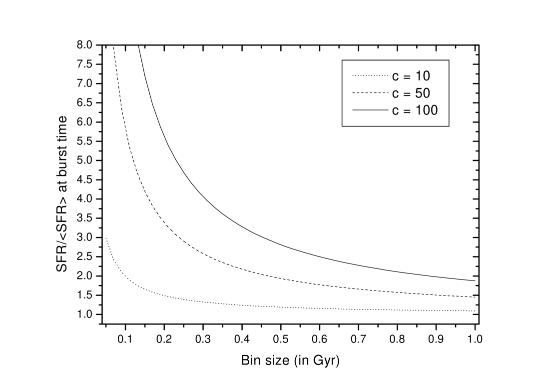
Figure 10: The evanescence of a strong short-lived star formation burst due to the bin size. A star formation burst, lasting $10^{7}$ yr, and with varying intensity (10, 50 and 100 times more intense than the average star formation rate) was considered. The plot shows the value of the relative birthrate at the time of a burst It can be seen that for an age bin similar to that used throughout this paper, namely 0.4 Gyr, even the most strong and narrow burst would be represented by a feature not exceeding 3.5 in units of relative birthrate.

In the case of our galaxy, the bin size presently cannot be smaller than 0.4 Gyr. This is caused by the magnitude of the age errors. We are then limited to features whose relative birthrate will be barely greater than 3.0, especially taking into consideration that the star formation in a spiral galaxy is more or less well distributed during its lifetime. Therefore, in a plot with bin size of 0.4 Gyr, relative birthrates of 2.0 are in fact big events of star formation.

A conclusive way to avoid these mistakes is to calculate the expected fluctuations of a constant SFH in the plots we are using. We have calculated the Poisson deviations for a constant SFH composed by 552 stars. In Figure 11 we show the 2$\sigma$ lines (dotted lines) limiting the expected statistical fluctuations of a constant SFH.

The Milky Way SFH, in this Figure, is presented with two sets of error bars, corresponding to extreme cases. The smallest error bars correspond to Poisson errors ($\pm\sqrt{N}$, where $N$ is the number of stars in each metallicity bin). The thinner longer error bar superposed on the first shows the maximum expected error in the SFH, coming from the combination of counting errors, IMF errors and scale height errors. These last two errors were estimated from Figures 4 and 5. The contribution of the scale height errors are greatest at an age of 3.0 Gyr, due to the steep increase of the scale heights around solar-mass stars. The effect of the IMF errors are the smallest, but grows in importance for the older age bins.

From the comparison of the maximum expected fluctuations of a constant SFH and the errors in the Milky Way SFH, it is evident that some trends are not consistent with a constant history, particularly bursts A and B, and the AB gap. We can conclude that the irregularities of our SFH cannot be caused by statistical fluctuations.

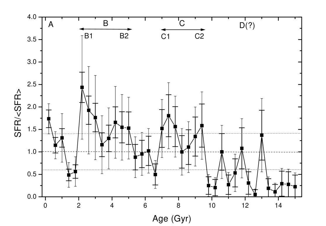
Figure 11: Star formation rate with counting errors. The error bars correspond to an error of $\pm\sqrt{N}$, where $N$ is the number of stars found in each age bin. The dotted lines indicate the 2$\sigma$ variations around a constant SFR for a sample having 552 stars. The labels over the peaks are the same as in Figure 8.

4.2 The uncertainty introduced by the age errors

The age error affects more considerably the duration of the star formation events, since they tend to scatter the stars originally born in a burst. We can expect that this error could smear out peaks and fill in gaps in the age distribution. A detailed and realistic investigation of the statistical meaning of our bursts has to be done in the framework of our method, following the observational data as closely as possible. In the case of the Milky Way, the input data is provided by the age distribution. We have supposed that this age distribution is depopulated from old objects, since some have died or left the galactic plane. Our method to find the SFH makes use of corrections to take into account these effects. However, some features in the age distribution could be caused rather by the incompleteness of the sample. These would propagate to the SFH giving rise to features that could be taken as real, when they are not.

Thus, if we want to differentiate our SFH from a constant one, we must begin with age distributions, generated by a constant SFH, depopulated in the same way that the Galactic age distribution. With this approach, we can check if the SFH presented in Figure 8 can be produced by errors in the isochrone ages in conjunction with statistical fluctuations of an originally constant SFH.

We have done a set with 6000 simulations to study this. Each simulation was composed by the following steps:

1. A constant SFH composed by 3000 ‘stars’ was built by randomly distributing the stars from 0 to 16 Gyr with uniform probability.

2. The stars are binned at 0.2 Gyr intervals. For each bin, we calculate the number of objects expected to have left the main sequence or the galactic plane. This corresponds to the number of objects which we have randomly eliminated from each age bin. The remaining stars (around 600-700 stars at each simulation) were put into an ‘observed catalogue’.

3. The real age of the stars in the ‘observed catalogue’ is shifted randomly according to the average errors presented in Figure 5 of Paper I. After that, the ‘observed catalogue’ looks more similar to the real data.

4. The SFH is then calculated just as it was done for the disk. From each SFH the following information is extracted: dispersion around the mean, amplitude and age of occurrence of the most prominent peak, amplitude and age of occurrence of the deepest lull.

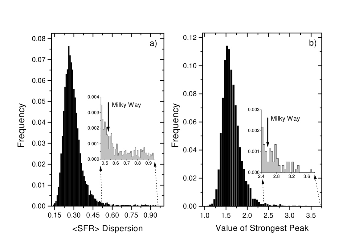
Figure 12: Distribution of parameters from 6000 simulations, using the scale heights from Scalo (scalo (1986)). The left panel shows the dispersions around the mean SFH, while the right panel gives the value of the most prominent peak. In all the plots, the arrow indicates the corresponding value for the Milky Way SFH.

One of the problems that we have found is that due to the size of the sample, and the depopulation caused by stellar evolution and scale height effects, the SFH always presents large fluctuations beyond 10 Gyr. These fluctuations are by no means real. They arise from the fact that in the observed sample (for the case of the simulations, in the ‘observed catalogue’), beyond 10 Gyr, the number of objects in the sample is very small, varying from 0 to 2 stars at most. In the method presented in the subsections above, we multiply the number of stars present in the older age bins by some factors to find the number of stars originally born at that time. This multiplying factor increases with age and could be as high as 12 for stars older than 10 Gyr; this way, by a simple statistical effect of small numbers, we can in our sample find age bins where no star was observed neighbouring bins where there are one or more stars. And, in the recovered SFH, this age bin will still present zero stars, but the neighbouring bins would have their original number of stars multiplied by a factor of 12. This introduces large fluctuations at older age bins, so that all statistical parameters of the simulated SFHs were calculated only from ages 0 to 10 Gyr.

In Figure 12, we present two histograms with the statistical parameters extracted from the simulations. The first panel shows the distribution of dispersions around the mean for the 6000 simulations. The arrow indicates the corresponding value for the Milky Way SFH. The dispersion of the SFH of our Galaxy is located in the farthest tail of the dispersion distribution. The probability of finding a dispersion similar to that of the Milky Way is lower than 1.7%, according to the plot. In other words, we can say, with a significance level of 98.3%, that the Milky Way SFH is not consistent with a constant SFH.

In panel b of Figure 12, a similar histogram is presented, now for the value of the most prominent peak that was found in each simulation. In the case of the Milky Way, we have B1 peak with $b=2.5$. Just like the previous case, it is also located in the tail of the distribution. From the comparison with the values of the highest peaks that could be caused by errors in the recovering of an originally constant SFH, we can conclude with a significance level of 99.5% that our Galaxy has not had a constant SFH.

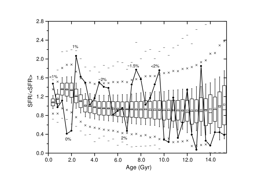
Figure 13: Box charts showing the results of the 6000 simulations, using Holmberg & Flynn (holmberg (2000))’s scaleheights. The horizontal lines in the box give the 25th, 50th, and 75th percentile values. The error bars give the 5th and 95th percentile values. The two symbols below the 5th percentile error bar give the 0th and 1st percentile values. The two symbols above the 95th percentile error bar give the 99th and 100th percentiles. The square symbol in the box shows the mean of the data. Superimposed, the Milky Way SFH is shown. From the comparison with the distribution of results at each age bin, the probability to find each particular event in a constant SFH can be calculated. The numbers besides the major events give the probabilities for their being fluctuations of a constant SFH.

The use of Holmberg & Flynn (holmberg (2000)) scale heights in the simulations increases these significance levels to 100% and 99.9%, respectively.

These significance levels refer to only one parameter of the SFH, namely the dispersion or the highest peak. For a rigorous estimate of the probability of finding a SFH like that presented in Figure 11, from an originally constant SFH, one has to calculate the probability to have neighbouring bins with high star formation, followed by bins with low star formation, as a function of age. This can be calculated approximately from Figure 13, where we show box charts with the results of the 6000 simulations. Superimposed on these box charts, we show the SFH, now calculated with Holmberg & Flynn (holmberg (2000))’s scale heights. For the sake of consistency, the simulations shown in the figure also use these scale heights, but we stress that the same quantitative result is found using Scalo’s scale heights.

A lot of information can be drawn from this figure. First, it can be seen that a typical constant SFH would not be recovered as an exactly ‘constant’ function in this method. This is shown by the boxes with the error bars which delineate 2$\sigma$-analogous to those lines shown in Figure 11. The boxes distribute around unity, but shows a bump between 1 to 2 Gyr, where the average relative birthrate increases to 1.4. This is an artifact introduced by the age errors. In each individual simulation, the number of stars scattered off their real ages increases as a function of the age. In the recovered SFH there will be a substantial loss of stars with ages greater than 15 Gyr, since they are eliminated from the sample (note that originally, these stars would present ages lower than 15 Gyr, and just after the incorporation of the age errors they resemble stars older than it). This decreases the average star formation rate with respect to the original SFH, and the proportional number of young stars increases, because they are less scattered in age due to errors. This gives rise to a distortion in the expected loci of constant SFHs. Note also the increase in the $2\sigma$-region as we go towards older ages, reflecting the growing uncertainty of the chromospheric ages.

The diagram allows a direct estimate of the probability for each feature found in the Milky Way SFH be produced by fluctuations of a constant SFH. The box charts gives the distribution of relative birthrates in each age bin. An average probability for the major events of our SFH are shown in Figure 13, besides the features under interest. Rigorously speaking, the probability for the whole Milky Way SFH be constant, not bursty, can be estimated by the multiplication of the probability of the individual events in this Figure. It can be clearly seen that it is much less than the 2% level we have calculated from only one parameter of the SFH. Particularly, note that the AB gap has zero probability to be caused by a statistical fluctuation. All of theses results show that the Milky Way SFH was by no means constant.

4.3 Flattening and Broadening of the Bursts

Since the errors in the chromospheric ages are not negligible, a sort of smearing out must be present in the data. Due to this, a star formation burst found in the recovered SFH must have been originally much more pronounced. This mechanism probably affects much more older bursts, since the age errors are greater at older ages and the depopulation by evolutionary and scaleheight effects is more dramatic. We can assume that if we found a feature like a burst at say 8 Gyr ago, this probably was much stronger in order to be preserved in the recovered SFH.

The first aspect we want to show is that the errors produce a significant flattening of the original peaks. To do so, we use simulations of a SFH composed by a single burst over a constant star formation rate. The ‘burst’ is characterized by occurring at age $\tau$, having intensity $c$ times the value of the constant star formation rate, and lasting 1 Gyr. We want to know the fraction of the burst that is recovered, as a function of age and of the burst intensity.

We have performed 50 simulations for each pair $(\tau,c)$, with around 3000 stars in each simulation. A summary of these simulations is shown in Figure 14. In all the panels (for varying $c$), the fraction of the recovered burst is high for recent bursts and falls off smoothly until 8-9 Gyr, when it begins to become constant. This stabilization reflects the predominance of the statistical fluctuations, since the recovered fraction is the same, regardless of the age of occurrence. What happens is that the burst becomes more or less undistinguished from the fluctuations. From this we can conclude that it is more difficult to find bursts older than 8-9 Gyr, irrespective of its original amplitude.

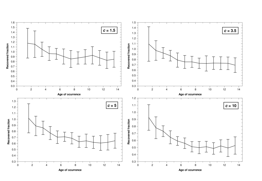
Figure 14: Recovered fractions for a SFH composed of a single burst superimposed on a constant rate. The ‘burst’ is characterized by occuring at age $\tau$, having intensity $c$ times the value of the constant star formation rate, and lasting 1 Gyr. We show the cases for $c=$ 1.5, 3.5, 5 and 10. In all the plots, the abscissa indicates the age $\tau$ where the burst happened. The fraction recovered in the first 2 Gyr of age is greater than unity, due to the same problem that distorted the $2\sigma$ loci of the constant SFHs in Figure 13 (see text).

A second problem in the method is the broadening of the bursts. This depends sensitively on the age at which the burst occurs, and the results are even more dramatic. To illustrate this, another set of simulations was done. We consider now a SFH composed of a single burst, of 1000 stars, lasting 0.4 Gyr. No star formation occurs except during the burst. We vary the age of occurrence from 0.3 Gyr to 6 Gyr ago. Just one simulation was done for each age of occurrence, since we are only looking for the magnitude of the broadening introduced by the errors, so the exact shape of the recovered SFH does not matter. The recovered SFHs are shown in Figure 15. Only the younger bursts are reasonably recovered. The burst at 6 Gyr can still be seen, although many of its stars has been scattered over a large range of ages.

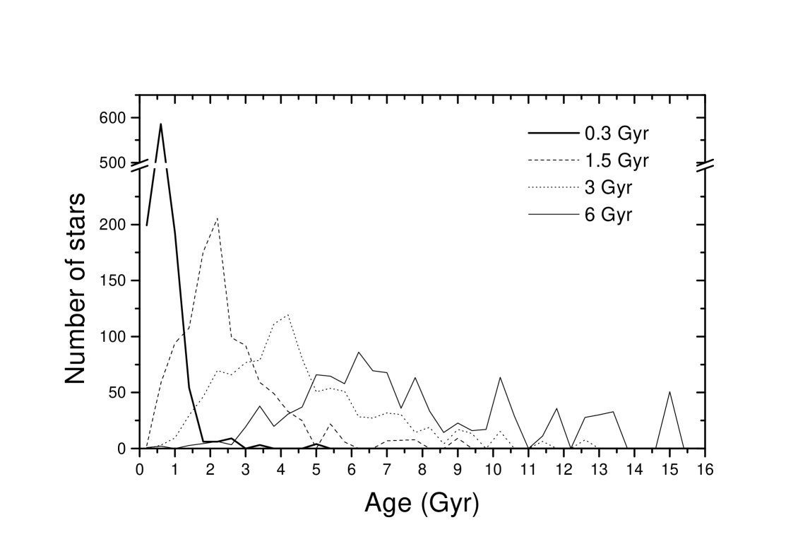
Figure 15: Recovered SFHs for an original SFH composed of a single burst of 1000 stars. The curves show examples of how these bursts are broadened, depending on their age of occurrence, due to age errors.

5 Comparison with other constraints

5.1 The SFH driving the chemical enrichment of the disk

On theoretical grounds, there should be a correlation between the SFH and the the age–metallicity relation (hereafter AMR). The increase in the star formation leads to an increase in the rate at which new metals are produced and ejected into the interstellar medium. The correlation is not a one-to-one, since the presence of infall and radial flows can also affect the enrichment rate of the system. Moreover, the enrichment rate is constrained by the amount of gas into which the new metals will be diluted. Nevertheless, it is interesting to see whether the AMR we have found in Paper I is consistent with the SFH derived from the same sample, especially because, to our knowledge, this was never tried before.

From the basic chemical evolution equations (Tinsley tinsley (1980)), for a closed box model (i.e., no infall), the link between the AMR and the SFH can be written as

$${{\rm d}Z\over{\rm d}t}(t)\propto{\psi(t)\over m_{g}(t)},$$ (11)

where $Z(t)$ gives the AMR, expressed by absolute metallicity, $\psi(t)$ is the SFH as in equation (1), and $m_{g}(t)$ is the total gas mass of the system, in units of $M_{\odot}$ pc^-2.

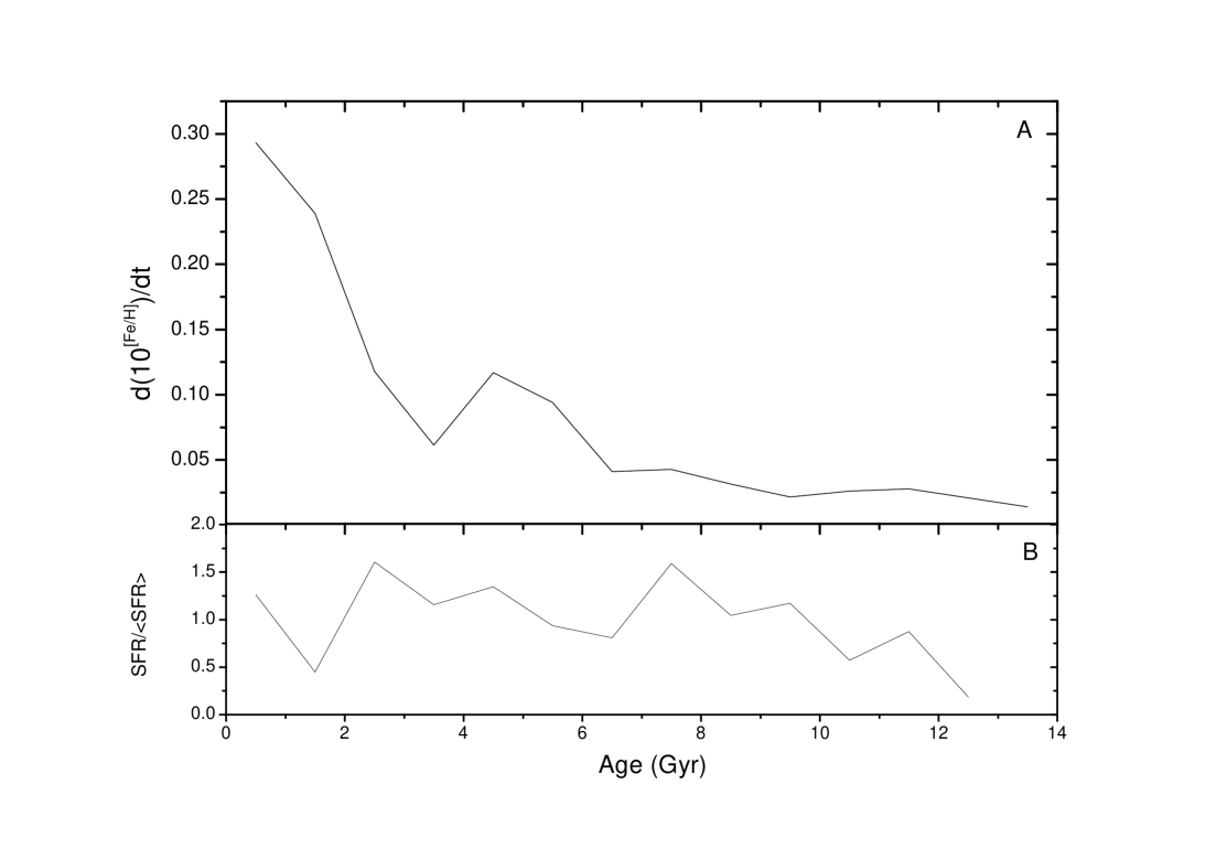
Figure 16: Comparison between the metal-enrichment rate (defined as the derivate in time of the AMR, expressed by absolute metallicity $Z$), and the SFH. On theoretical grounds both quantities should be correlated, and it should give a test to the reliability of the SFH. In practice, the magnitude of the errors in both functions still hinders the application of this test.

According to this equation, bursts in the SFH are echoed through an increase of the metal-enrichment rate. Certainly, this is particularly true when the metallicity is measured by an element produced mostly in type II supernovae, like O. The gas mass can dilute more or less the enrichment, changing the proportionality between it and the SFH, at each age, but will not destroy the relationship. On the other hand, the intrinsic metallicity dispersion of the interstellar medium can certainly somewhat obscure this proportionality, especially if it were as big as the AMR by Edvardsson et al. (Edv (1993), hereafter Edv93) suggests.

In Figure 16, we show a comparison between the metal-enrichment rate (top panel) with the SFH (bottom panel). The enrichment rate increases substantially in the last 2 Gyr, which could be a suggestion for a recent burst of SFH. However, the agreement between both functions seems very poor. There is a peculiar bump in the enrichment rate between 4 and 6 Gyr, which is coeval to a feature in the SFH, but most probably this is mere coincidence.

Although we have used iron as a metallicity indicator, which invalidates Equation (11), due to non recycling effects, we are not sure whether the situation would be improved by using O. The errors in both the AMR and SFH are still big enough to render such a comparison extremely uncertain. However, it can be a test to be done with improved data. The more important result for chemical evolution studies is that, provided that we know accurately both functions, the empirical AMR and SFH will allow an estimate of the variation of the gas mass with time, which could lead to an estimate of the evolution of the infall rate. Future studies should attempt to explore this tool.

5.2 Scale length of the SFH

The stars in our sample are all presently situated within a small volume of about 100 pc radius around the Sun. The star formation history derived from these stars is nevertheless applicable to a quite wide section of the Galactic disk, since the stars which are presently in the Solar neighbourhood have mostly arrived at their present positions from a torus in the disk concentric with the Solar circle.

We have investigated how wide this section of disk is by integrating the equations of motion for 361 stars of the ‘kinematic sample’ (see Paper I) within a model of the Galactic potential. The potential consists of a thin exponential disk, a spherical bulge and a dark halo, and is described in detail in Flynn et al. (flynn1996 (1996)). For each star we determine the orbit by numerical integration, and measure the peri- and apogalactic distances, $R_{p}$ and $R_{a}$ and the mean Galactocentric radius, $R_{m}=(R_{p}+R_{a})/2$ for the orbit (cf. Edvardsson et al. Edv (1993)).

The distribution of $R_{m}$ is shown in Figure 17. Most of the stellar orbits have mean Galactocentric radii within 2 kpc of the Sun (here taken to be at $R_{\odot}=8$ kpc), i.e. $6<R_{m}<10$ kpc. Very few stars in the sample are presently moving along orbits with mean radii beyond these limits.

As discussed by Wielen, Fuchs and Dettbarn (WFD (1996)), due to irregularities in the Galactic potential caused by (for example) giant molecular clouds and spiral arms, the present mean Galactocentric radius of a stellar orbit $R_{m}(t)$ at time $t$ does not bear a simple relationship to the mean Galactocentric radius of the orbit on which the star was born $R_{m}(0)$. Wielen, Fuchs and Dettbarn describe the process by which stars are scattered by these irregularities as orbital diffusion, and show that over time scales of several Gyr, that one cannot reconstruct from $R_{m}$ the radius at which any particular star was born to better than a few kpc. This is of the same order as the width of the distribution of $R_{m}$ seen in Figure 17. We therefore conclude that our stars fairly represent the star formation history within a few kpc of the present Solar radius, $6<R_{m}<10$, or the “middle distance” regions of the Galactic disc. The SFH of the inner-disk/bulge, and the outer disk are not sampled.

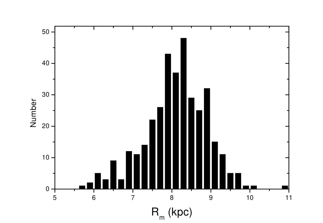
Figure 17: The histogram presents the mean galactocentric radius for the orbits of 361 stars presently located near the Sun. According to Binney & Sellwood (2000), these mean galactocentric radii indicate with good confidence the stellar birthplace radii. This shows that the SFH here derived is not a local history, but the average history over a significant part of the Milky Way disk.

However, Binney & Sellwood (binney (2000)) have criticized this conclusion. They show that during the lifetime of a star, the guiding-center of its orbit can change generally by no more than 5%. In this scenario, the value of $R_{m}$ that we have calculated is close to the galactocentric radius of the star birthplace, and our star formation history would still be representative of a considerable fraction of the galactic disk, $7<R_{m}<9$.

Another important conclusion of kinematic studies it that the older is a feature in the SFH, the more damped it is recovered from the data, related to its original amplitude (see, for example, Meusinger 1991b ), since the stars formed by the burst will be scattered through a larger region. Hence, the younger bursts in our SFH are the most local features. This does not mean that they are most probably ‘local irregularities’. In time scales of 1-2 Gyr, the diffusion of stellar orbits homogenize any irregularities in the azimutal direction, so that the bursts would apply to the whole solar galactocentric annulus.

5.3 The Galaxy and the Magellanic Clouds

When evidences for an intermittent SFH in the Galaxy were first discovered, Scalo (scalo87 (1987)) proposed that they could have originated from interactions between the Galaxy and the Magellanic Clouds. Indeed, the Magellanic Clouds are known to have probably experienced some episodes of strong star formation for a long time. Butcher (acougueiro (1977)) first proposed that the bulk of star formation in the Large Magellanic Cloud (LMC) has occurred from 3-5 Gyr ago, by the analysis of the luminosity function of field stars. Stryker et al. (stryker1 (1981)) and Stryker (stryker2 (1983)) subsequently confirmed this result. In the last few years, additional studies have arrived almost at the same conclusions (Bertelli et al. bertelli (1992); Vallenari et al. 1996a ,b). Westerlund (wester (1990)) also remarked that the star formation in the LMC seems to have been very small from 0.7 to 2 Gyr ago. A very recent burst of star formation (around 150 Myr ago) was also found by the MACHO team (Alcock et al. todopau (1999)) from the study of the period distribution of 1800 LMC cepheids. Their analysis present compeling arguments favouring this hypothesis, as well as for the propagation of the star formation to neighbour regions.

However, these results have more recently been questioned, on the basis of colour-magnitude diagram synthesis. Some authors claim that important information on the SFH are provided by the part of the colour–magnitude diagram below the turnoff-mass, which could only be resolved with the most recent observations (Holtzman et al. vera_holtz (1997), holtz99 (1999), and references therein; Olsen xxx (1999)). These papers conclude that star formation in the LMC has been a continuous process over much of its lifetime.

Note that continuity in the SFH does not means constancy. Holtzman et al. (holtz99 (1999)) points that their method cannot constrain accurately the burstiness of the SFH in the LMC on small time scales, particularly for ages greater than 4 Gyr. Nevertheless, they show evidence for an increase in the star formation rate in the last 2.5 Gyr. Dolphin (dolphin (2000)) arrives to the same conclusion studying two different fields of the LMC, separated by around 2 kpc one from the other. The author recognizes that some large environment alteration must have triggered an era of star formation in our neighbour galaxy.

In spite of the controversy, it is impossible not to verify that some results on the SFH of the LMC are in apparently synchronism with some SFH events in the Milky Way disk. But this should be not really surprising. The Magellanic Clouds are satellites of our Galaxy, and past interactions between them were a rule, not an exception. Byrd & Howard (byrd (1992)) showed that a companion satellite, whose mass is larger than 1% of the primary galaxy, could excite large-scale tidal arms in the disk of the primary, and we know that spiral arms do induce, or at least organize, star formation. This number is to be compared with the mass ratio between our Galaxy and the Clouds which is 0.20 (Byrd et al. byrdetal (1994)). Besides direct tidal effects, the Clouds can produce a dynamical wake in the halo that distorts the disk (Weinberg weinberg (1999)). It is quite possible that such an effect could also enhance the star formation in the disk (M. Weinberg, private communication).

Additional evidence comes from dynamical studies of the Magellanic Clouds. Several groups have worked on the derivation of their orbits around the Galaxy. The full orbit of the Magellanic Clouds are still unknown, but there is some agreement in the published works. The most important is that all of these works conclude that the most recent close encounter between the Clouds and the Milky Way has occurred 0.2-0.5 Gyr ago, which was the closest encounter through the entire history of the system (however, Holtzman et al. holtz99 (1999) mention an unpublished work by Zhao in which the last perigalacticon occurred 2.5 Gyr ago). Murai & Fujimoto (murai (1980)) calculated that other close encounters have occurred 1.5, 2.6 and 7.5 Gyr ago. Gardiner et al. (gardiner (1994)) revisited Murai & Fujimoto (murai (1980))’s model and recalculated the epochs of the close encounters as around 1.6, 3.4, 5.5, 7.6 and 10 Gyr ago. However, Lin et al. (lin (1995)) have found different values: 2.6, 5.3, 8.4 and 11.8 Gyr ago.

From these results we can tentatively assume that, in the last 12 Gyr, the Clouds have had at most six close encounters with the Milky Way occurring more or less at 0.2-0.5, 1.4-1.5, 2.6-3.4, 5.3-5.5, 7.5-8.4 and 10-11.8 Gyr ago. Some of these encounters are not predicted by all the authors, while some are in good agreement. For the sake of simplicity, we will refer to these encounters as I, II, III, IV, V and VI, respectively.

There are similarities between the time of close encounters and the events of our derived SFH. In Figure 18 we show the epoch of these encounters superimposed over our SFH. We can associate burst A with encounter I, peak B1 with encounter III, and peak C1 with encounter V. It is not unlikely that peak B2 could also be associated with encounter IV. On the other hand, encounter VI probably cannot be responsible for any of the features found beyond 9 Gyr, since it occurs in an age range where the SFH is highly uncertain and subject to random fluctuations.

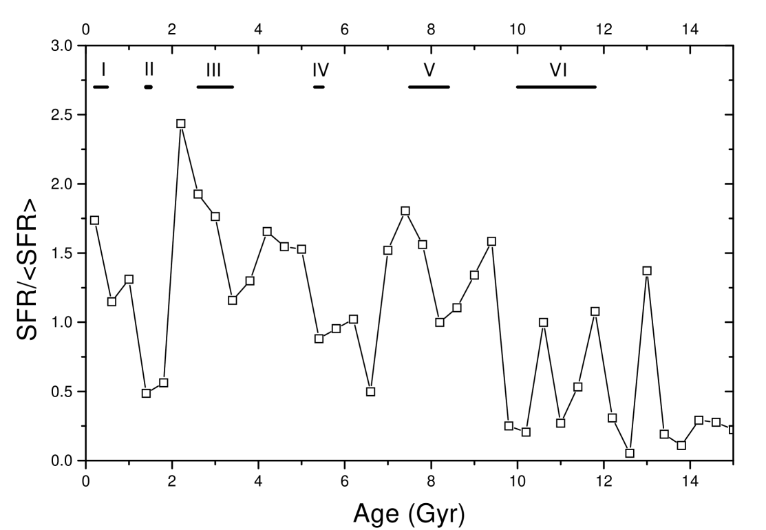
Figure 18: Star formation history compared with the times of close encounters between the Galaxy and the Magellanic Clouds.

A significant exception to the rule is encounter II. It is thought to have happened in the middle of the AB gap. It seems strange to think that a close encounter between interacting galaxies could suppress the star formation. Other mechanism should be responsible for the gap. On the other hand, Lin et al. (lin (1995)) have not found such an encounter. In fact, these authors predict that by this time, the Clouds would be located in their apogalacticon, more than 100 kpc away.

Although the comparison is very premature, we conclude that the data on the age distribution and orbits of the Magellanic Clouds present some agreement with the Miky Way SFH. Have the bursts of star formation in the Milky Way been produced by interaction with its satellite galaxies? The comparison above certainly points to this possibility, that deserves more investigations to be properly answered, since there is still much uncertainty in the Magellanic Clouds close encounters, as well as on the chronologic scale of the chromospheric ages.

6 The features of the Milky Way SFH

We now can return to the discussion of the meaning of each feature found in the SFH derived in section 3.

6.1 Burst A

The most recent star formation burst is also the most likely burst to have occurred, since it has occurred in the very recent past, and so is less affected by the age errors. A recent enhancement in the SFH is also present in nearly all previous investigations of the SFH (Scalo scalo87 (1987); Barry barry (1988); Gómez et al. gomez (1990); Noh & Scalo noh (1990); Soderblom et al. soder91 (1991); Micela et al. micela (1993); Rocha-Pinto & Maciel RPM97 (1997); Chereul et al. chereul (1998)), and is consistent with the distribution of spectral types in class V stars (Vereshchagin & Chupina veresh (1993)). It is not present in the isochrone age distributions (Twarog twar (1980); Meusinger 1991a ) most probably due to the difficulty to measure ages for stars near the zero-age main sequence, where we expect to find the components of this burst in a HR diagram.

We can conclude with confidence that it is a real feature of the SFH. However, being the youngest, it is also the most local feature, because the younger stars have had no time to diffuse to larger distances from their birthsites. Thus, we cannot be sure (from out data only) whether this feature applies to the Milky Way as a whole.

On the other hand, it is known that the Large Magellanic Cloud appears to have experienced also a recent burst of star formation (Westerlund wester (1990); Alcock et al. todopau (1999)) which is very well represented by its young population of open clusters, cepheids, OB associations and red supergiants. At the time of this burst, both galaxies have been closer than ever in their history (Lin et al. lin (1995)). This suggests that burst A could be caused by tidal interactions between our Galaxy and the LMC.

6.2 AB gap

A substantial depression in the star formation rate 1-2 Gyr ago was found by many studies, beginning with Barry (barry (1988); see also the SFH derived from the massive white dwarf luminosity function derived by Isern et al. isern (1999)). This gap appears, although not directly, in the chromospheric age distribution (the so-called Vaughan-Preston gap) and in the spectral type distribution, between A and F dwarfs (Vereshchagin & Chupina veresh (1993)). A quiescence between 1 and 2 Gyr is also visible in Chereul et al. (chereul (1998)), in their study of the kinematical properties of A and F stars in the solar neighbourhood.

This feature has been present in all steps of our work, from the initial age distribution in Figure 1 to the SFH. Note that the volume corrections have deepened this lull, but it has not changed its duration.

The AB gap is likely to have lasted for a billion years. Previous studies have given a more extended duration for it, but we believe that it was caused by the use of a highly incomplete sample, together with a chromospheric age calibration that does not account for the different chemical composition of the stars. Since it is a relatively recent feature, it only samples birthsites over a radial length scale of 1-2 kpc.

6.3 Burst B

The small lull between the peaks B1 and B2 is not present in the initial age distribution (Figure 1), appearing only after the volume corrections. It is very narrow, which could be most probably caused by hazardous small weights of the stars in these age bins, during the volume correction. This is why we have presently no means to distinguish burst B from a single burst or an unresolved double burst. At its age of occurrence, considerable broadening of the original features is expected. Either way, our simulations give strong support to this feature.

Previous studies have found star formation enhancements around 4 Gyr ago (Scalo scalo87 (1987); Barry barry (1988); Marsakov et al. marsakov (1990); Noh & Scalo noh (1990); Soderblom et al. soder91 (1991); Twarog twar (1980); Meusinger 1991a ). Note that a strong concentration of stars around this age can also be found in the age distribution of Edv93’s stars, that we show in Figure 19.

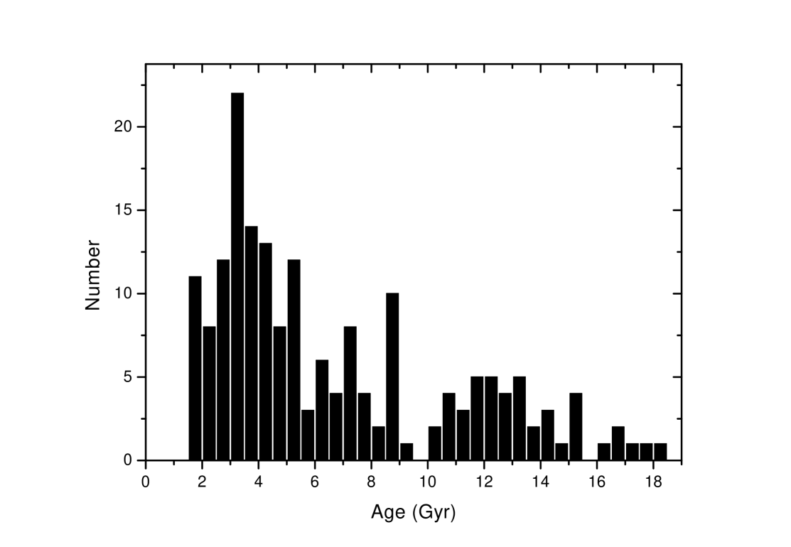
Figure 19: Age distribution of Edv93’s sample. The concentration of stars around 4 Gyr shows evidence of burst B. The lack of objects with ages lower than 2 Gyr is not an evidence of the AB gap, since Edv93 avoided the inclusion of very young stars due to the difficulty to measure an isochrone age for them.

A significant exception is the SFH found by some of us (Rocha-Pinto & Maciel RPM97 (1997)). This paper suggests that burst B would be much smaller than the preceding burst C. To find the SFH, Rocha-Pinto & Maciel used a method to extract information from the G dwarf metallicity distribution (Rocha-Pinto & Maciel RPM96 (1996)) aided by the AMR (see also Prantzos & Silk prantzos (1998)). The authors have used several AMRs from the literature and different SFHs were found for each AMR. The SFHs recovered with the AMR from Twarog (twar (1980)) and Meusinger et al. (meu (1991)) were preferred compared to that found with Edvardsson et al. Edv (1993) (hereafter Edv93) AMR. To be consistent with our present result, we need to compare the present SFH with that coming from Rocha-Pinto & Maciel’s method for an AMR similar to that found from our sample (paper I). Our AMR now looks very similar to the mean points of Edv93’s AMR. Rocha-Pinto & Maciel (RPM97 (1997)) have found, using Edv93’s AMR, that Burst B could have around the same intensity as burst C, and also a narrow AB gap lasting 1 Gyr at most. Figure 20 shows a comparison between their SFH (for Edv93’s AMR) and the present history binned by 1 Gyr intervals.

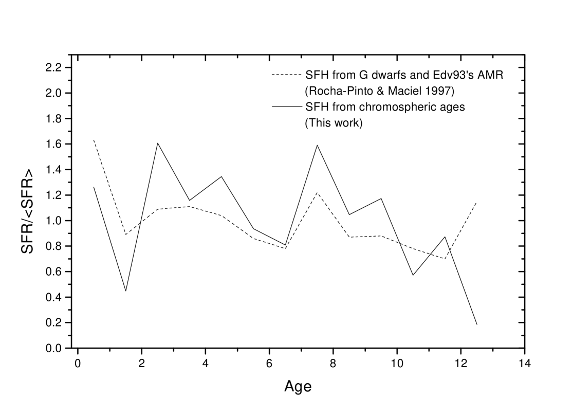
Figure 20: Comparison between Rocha-Pinto & Maciel (RPM97 (1997))’s SFH (for Edv93’s AMR) and the present chromospherically-based SFR binned by 1 Gyr intervals.

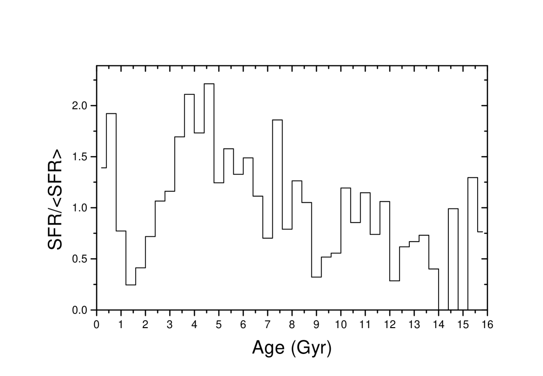
Figure 21: Results from an example simulation to show how the observed features: Burst A and B and AB gap could be caused by two bursts separated by a lull of star formation. See text for description of the original SFH used in this simulation.

6.4 BC gap and Burst C

The existence of the BC gap is directly linked with how much credit we are going to give to Burst C. From Figure 15, one could say that no burst could be found around 8-9 Gyr, and all supposed features are artificial patterns created by statistical fluctuations. To reinforce this theoretical expectation, we have done a simulation to show how the features above could be formed by a bursty SFH. We have considered a SFH composed by three bursts, one occurring at 0.3 Gyr, lasting 0.2 Gyr, and the other at 4 Gyr, also lasting 0.2 Gyr, and the last ocurring at 9 Gyr, lasting 0.5 Gyr. The first burst and the last burst are composed by 300 stars, while the second burst is three times more intense. The star formation at other times is assumed to be highly inefficient, forming only 60 more stars at the whole lifetime of the galaxy. The recovered SFR is shown in Figure 21. Although the two more recent bursts can be well recovered, there is no sign of burst C at 9 Gyr. We have tried other combinations between the amplitude and time of occurrence of them, but in all cases the stars of burst C were much scattered from its original age.

If on theoretical grounds there is no convincing arguments to accept the existence of burst C, the same does not occur on observational grounds. This puzzling situation comes from the fact that burst C has appeared in a number of studies that have used not only different samples, but also different methods (Barry barry (1988); Noh & Scalo noh (1990); Soderblom et al. soder91 (1991); Twarog twar (1980); Meusinger 1991a ; Rocha-Pinto & Maciel RPM97 (1997)). And it appears double-peaked in some of them, as we saw in section 3.

The magnitude of the age errors prevents us from assigning a good statistical confidence to this particular feature.

However, it is not implausible that we have overestimated the age errors. A decrease of 0.05 dex in the age errors could alleviate the situation and allow the identification of peaks (although highly broadened) younger than 10 Gyr, which would suggest that burst C is a real feature. A better estimate of the age errors would not create new bursts, or flatten the recovered SFH in these age bins, but would give confidence limits for the ages where the features found are likely to be real and not just artifacts.

6.5 Burst D

The so-called burst D was proposed by Majewski (majewski (1993)), as a star formation event that would be responsible for the first stars of the disk, before the formation of the thin disk.

A superficial look at Figure 8 could give us the impression that the peaks beyond 11 Gyr were remnants of this predicted burst. However, as we have shown above, it is presently impossible to recover the SFH correctly at this age range, even if our age errors are overestimated by as much as 0.05 dex. The SFH at older ages are dominated by fluctuations, superimposed on the original strongly broadened structures, in such a way that it is imposible to disentangle statistical fluctuations from real star formation events.

Theoretically, patterns as old as 13 Gyr could be found in the SFH, provided that they occurred not very close to younger ones, if the age errors were decreased by 0.10 dex, but that is hardly possible to be attained at the present moment since it would need to be of the order of magnitude of the error in the $\log R^{\prime}_{\rm HK}$ index.

For these reasons, we give no credit to the peaks beyond 11 Gyr in Figure 8. If burst D has ever occurred, probably the present chromospheric age distribution is not an efficient tool to find its traces.

7 The shape of the chromospheric activity–age relation

Soderblom et al. (soder91 (1991)) argued that the interpretation of the chromospheric activity distribution as evidence for a non-constant SFH is premature. Particularly, the authors have shown that the observations do not rule out a non-monotonic chromospheric activity–age relation, even considering that the simplest fit to the data is a power-law, like the one we used.

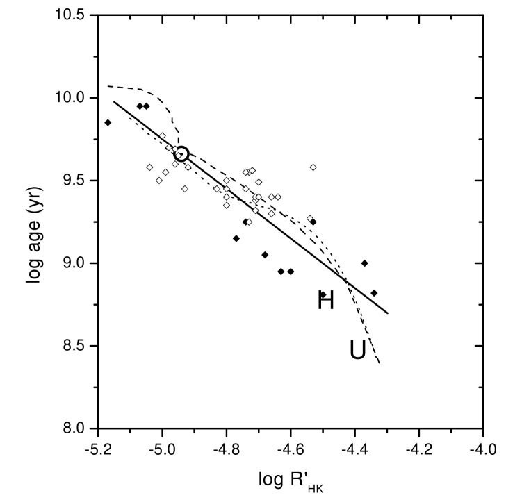
Figure 22: Comparison between the chromospheric activity–age relation we have used throughout this paper (solid line), the constant-sfr calibration proposed by Soderblom et al. (dotted line) and the constant-sfr calibration from our sample (dashed line). The data and symbols are the same from Soderblom et al. (soder91 (1991)): $\odot$, the sun; H, Hyades; U, Ursa Major Group; open diamonds, field F dwarfs; filled diamonds, binaries.

Presently, there is good indication that the chromospheric activity of a star is linked with its rotation, and that the rotation rate decreases slowly with time. However, it is unknown how exactly the chromospheric activity is set and how it develops during the stellar lifetime. The data show that there is a chromospheric activity–age relation, but the scatter is such that it is not presently possible to know whether the chromospheric activity decreases steadily with time, or there are plateaux around some ‘preferred’ activity levels. There is a possibility that the clumps we are seeing in the chromospheric age distribution (which are further identified as bursts) are artifacts produced by a monotonic chromospheric activity–age relation.

To keep the constancy of the SFH, Soderblom et al. (soder91 (1991)) proposed an alternative chromospheric activity–age relation that is highly non-monotonic. We have checked this constant-sfr calibration with our sample, but the result is not a constant sfr. This is expected, since there are many differences in the chromospheric samples used by Soderblom (soder (1985)) and Soderblom et al. (soder91 (1991)) and the one we have used (see our Figure 11 in Paper I). We have calculated a new constant-sfr calibration, in the way outlined by Soderblom et al. (soder91 (1991)). We have used 328 stars from our sample (just the stars with solar metallicity, to avoid the metallicity dependence of $\log R^{\prime}_{\rm HK}$), with weights given by the volume correction (to account for the completeness of the sample) and using the scale height correction factors to take into account the disk heating.

Figure 22 compares the chromospheric activity–age relation we have used (solid line) with the constant-sfr calibration proposed by Soderblom et al. (dotted line) and the constant-sfr calibration from our sample (dashed line). The data and symbols are the same from Soderblom et al. (soder91 (1991)). Both constant sfr calibrations agree reasonably well for the active stars, but deviate somewhat for the inactive stars. This is caused by the fact that to be consistent with a constant sfr, the calibration must account for the increase in the relative proportions of inactive to active stars, especially around $\log R^{\prime}_{\rm HK}=-4.90$, after the survey of HSDB. Note that, our constant-sfr chromospheric activity–age relation is still barely consistent with the data and cannot be ruled out. There are few data for stars older than the Sun in the plot, and it is not possible to know whether the plateau for $\log R^{\prime}_{\rm HK}<-5.0$ in this calibration is real or not.

We acknowledge that, given no other information, it is a subjective matter whether to prefer a complex star formation history or a complex activity-age relation. Nevertheless, there are numerous independent lines of evidence that also point to a bursty star formation history; the most recent and convincing is the paper by Hernandez, Valls-Gabaud & Gilmore (valls (2000)). They use a totally different technique (colour–magnitude diagram inversion) and find clear signs of irregularity in the star formation. In section 6, we listed several other works that indicate a non-constant star formation history, and the majority of them use different assumptions and samples. Strongly discontinuous star formation histories are also found for some galaxies in the Local Group (see O’Connell oconnell (1997)), in spite of the initial expectations during the early studies of galactic evolution that these galaxies should have had smooth star formation histories.

For all these methods to give the same sort of result, all the different kinds of calibrations would have to contain complex structure. It is simpler to infer that the star formation history is the one that actually has a complex structure. We think that when several independent methods all give a similarly bursty star formation history (although with different age calibrations, so they do not match exactly), our conclusion is supported over the irregular activity-age but constant star formation rate solution.

8 Conclusions

A sample composed of 552 stars with chromospheric ages and photometric metallicities was used in the derivation of the star formation history in the solar neighbourhood. Our main conclusions can be summarized as follow:

1. Evidence for at least three epochs of enhanced star formation in the Galaxy were found, at 0-1, 2-5 and 7-9 Gyr ago. These ‘bursts’ are similar to the ones previously found by a number of other studies.

2. We have tested the correlation between the SFH and the metal-enrichment rate, given by our AMR derived in Paper I. We have found no correlation between these parameters, although the use of Fe as a metallicity indicator, and the magnitude of the errors in both functions can still hinder the test.

3. We examined in some detail the possibility that the Galactic bursts are coeval with features in the star formation history of the Magellanic Clouds and close encounters between them and our Galaxy. While the comparison is still uncertain, it points to interesting coincidences that merit further investigation.

4. A number of simulations was done to measure the probability for the features found to be consistent with a constant SFH, in face of the age errors that smear out the original features. This probability is shown to decrease for the younger features (being nearly 0% for the quiescence in the SFH between 1-2 Gyr), such that we cannot give a strong assertion about the burst at 7-9 Gyr. On the other hand, the simulations allow us to conclude, with more than 98% of confidence, that the SFH of our Galaxy was not constant.

There is plenty of room for improvement in the use of chromospheric ages to find evolutionary constraints. For instance, a reconsideration of the age calibration and a better estimate of the metallicity corrections could diminish substantially the age errors, which would not only improve the age determination but also give more confidence in the older features in the recovered SFH.

- (1) Alcock C., Allsman R.A., Alves D.R., 1999, AJ 117, 920
- (2) Bahcall J.N., Piran T., 1983, ApJ 267, L77
- (3) Barry D.C., 1988, ApJ 334, 446
- (4) Barry D.C., Cromwell R.H., Hege E.K., 1987, ApJ 315, 264
- (5) Bertelli G., Mateo M., Chiosi C., Bressan A., 1992, ApJ 388, 400
- (6) Binney J.J., Sellwood J.A., 2000, preprint (astro-ph/0003194)
- (7) Bressan A., Fagotto F., Bertelli G., Chiosi C., 1993, A&AS 100, 647
- (8) Butcher H., 1977, ApJ 216, 372
- (9) Byrd G., Howard S., 1992, AJ 103, 1089
- (10) Byrd G., Valtonen M., McCall M., Innanen K., 1994, AJ 107, 2025
- (11) Chereul E., Crezé M., Bienaymé O., 1998, A&A 340, 384
- (12) Dolphin A.E., 2000, MNRAS 313, 281
- (13) Donahue R.A., 1993, PhD Thesis, New Mexico State University
- (14) Donahue R.A., 1998, in Donahue R.A. and Bookbinder J.A., eds., Stellar Systems and the Sun, ASP Conf. Ser. 154, 1235
- (15) Edvardsson B., Anderson J., Gustafsson B., Lambert D.L., Nissen P.E., Tomkin J., 1993, A&A 275, 101 (Edv93)
- (16) Eggleton P.P., Fitchett M.J., Tout C.A., 1989, ApJ 347, 998
- (17) Fagotto F., Bressan A., Bertelli G., Chiosi C., 1994a, A&AS 104, 365
- (18) Fagotto F., Bressan A., Bertelli G., Chiosi C., 1994b, A&AS 105, 29
- (19) Flynn C., Sommer-Larsen J., Christensen P.R., 1996, MNRAS 281, 1027
- (20) Gardiner L.T., Sawa T., Fujimoto M., 1994, MNRAS 266, 567
- (21) Giménez A., Reglero V., de Castro E., Fernández-Figueroa M.J., 1991, A&A 248, 563
- (22) Gómez E.A., Delhaye J., Grenier S., Jaschek C., Arenou F., Jaschek M., 1990, A&A 236, 95
- (23) Haywood M., Robin A.C., Crézé M., 1997, A&A 320, 428
- (24) Hernandez X., Valls-Gabaud D., Gilmore G., 2000, preprint (astro-ph/0003113)
- (25) Henry T.J., Soderblom D.R., Donahue R.A., Baliunas S.L., 1996, AJ 111, 439 (HSDB)
- (26) Holmberg, J., Flynn C., 2000, in preparation
- (27) Holtzman J.A., Mould J.R., Gallagher III J.S., et al., 1997, AJ 113, 656
- (28) Holtzman J.A., Gallagher III J.S., Cole A.A., et al., 1999, AJ 118, 2262
- (29) Isern J., Hernanz M., Garcia-Berro E., Mochkovitch E., 1999, in 11th European Workshop on White Dwarfs, Solheim J.E., Meistas E.G., eds., ASP Series, Vol. 169, p. 408
- (30) Lin D.N.C., Jones B.F., Klemola A.R., 1995, ApJ 439, 652
- (31) Majewski S.R., 1993, ARA&A 31, 575
- (32) Marsakov V.A., Sheveler I.G., Suchkov A.A., 1990, ApSS 172, 51
- (33) Meusinger H., 1991a, ApSS, 181, 19
- (34) Meusinger H., 1991b, Astron. Nachr., 4, 231
- (35) Meusinger H., Reimann H.-G., Stecklum B., 1991, A&A, 245, 57
- (36) Micela G., Sciortino S., & Favata F., 1993, ApJ 412, 618
- (37) Miller G.E., Scalo J.M., 1979, ApJS, 41, 513
- (38) Murai T., Fujimoto M., 1980, PASJ 32, 581
- (39) Noh H.-R., Scalo J., 1990, ApJ 352, 605
- (40) O’Connell R.W., 1997, in Holt S.S., Mundy L.G. (eds.), Star Formation Near and Far, AIP Press, New York, 491
- (41) Olsen K.A.G., 1999, AJ 117, 2244
- (42) Prantzos N., Silk J., 1998, ApJ 507, 229
- (43) Rana N.C., Basu S., 1992, A&A 265, 499
- (44) Rocha-Pinto H.J., Maciel W.J., 1996, MNRAS 279, 447
- (45) Rocha-Pinto H.J., Maciel W.J., 1997, MNRAS 289, 882
- (46) Rocha-Pinto H.J., Maciel W.J., 1998, MNRAS, 298, 332
- (47) Rocha-Pinto H.J., Maciel W.J., Scalo J.M., Flynn C., 2000a, A&A, submitted (Paper I)
- (48) Rocha-Pinto H.J., Scalo J.M., Maciel W.J., Flynn C., 2000b, ApJ 531, L115
- (49) Scalo J.M., 1986, Fund. Cosm. Phys. 11, 1
- (50) Scalo J.M., 1987, in Thuan T.X, Montmerle T., and Tran Thanh Van, eds., Starbursts and Galaxy Evolution, Editions Frontières, Gif sur Yvette, 445
- (51) Scalo J.M., 1998, in Gilmore G., Howell D., eds., The Stellar Initial Mass Function, ASP Conf. Series 142, 201
- (52) Schaller G., Schaerer D., Meynet G., Maeder A., 1992, A&AS 96, 269
- (53) Soderblom D.R., 1985, AJ 90, 2103
- (54) Soderblom D.R., Duncan D.K., Johnson D.R.H., 1991, ApJ 375, 722
- (55) Stryker L.L., 1983, ApJ 266, 82
- (56) Stryker L.L., Butcher H.R., Jewell J.L., 1981, in IAU Colloquim 68: Astrophysical Parameters for Globular Cluters, Phillip A.G.D., Hayes D.S. (eds.), L. Davis Press, 225
- (57) Tinsley B.M., 1974, A&A 31, 463
- (58) Tinsley B.M., 1980, Fund. Cosm. Phys. 5, 287
- (59) Twarog B.A., 1980, ApJ 242, 242
- (60) Vallenari A., Chiosi C., Bertelli G., Ortolani S., 1996a, A&A 309, 358
- (61) Vallenari A., Chiosi C., Bertelli G., Aparicio A., Ortolani S., 1996b, A&A 309, 367
- (62) VandenBerg D.A., 1985, ApJS 58, 711
- (63) Vereshchagin S.V., Chupina N.V., 1993, Astron. Rep. 39, 808
- (64) Weinberg M.D., 1999, in The Third Stromlo Symposium: The Galactic Halo (ASP Conference Series), in press (astro-ph/9811204).
- (65) Westerlund B.E., 1990, A&AR 2, 29
- (66) Wielen R., Fuchs B., Dettbarn C., 1996, A&A 314, 438