Chemical enrichment and star formation in the Milky Way disk

Abstract

The age–metallicity relation of the solar neighbourhood is studied using a sample of 552 late-type dwarfs. This sample was built from the intersection of photometric catalogues with chromospheric activity surveys of the Mount Wilson group. For these stars, metallicities were estimated from uvby data, and ages were calculated from their chromospheric emission levels using a new metallicity-dependent chromospheric activity–age relation developed by Rocha-Pinto & Maciel (RPM98 (1998)). A careful estimate of the errors in the chromospheric age is made. The errors in the chromospheric indices are shown to include partially the effects of the stellar magnetic cycles, although a detailed treatment of this error is still beyond our knowledge. It is shown that the results are not affected by the presence of unresolved binaries in the sample. We derive an age–metallicity relation which confirms the mean trend found by previous workers. The mean metallicity shows a slow, steady increase with time, amounting at least 0.56 dex in 15 Gyr. The initial metallicity of the disk is around $-0.70$ dex, in agreement with the G dwarf metallicity distribution (Rocha-Pinto & Maciel RPM96 (1996)). According to our data, the intrinsic cosmic dispersion in metal abundances is around 0.13 dex, a factor of two smaller than that found by Edvardsson et al. (Edv (1993)). We show that chromospheric ages are compatible with isochrone ages, within the expected errors, so that the difference in the scatter cannot be caused by the accuracy of our ages and metallicities. This reinforces some suggestions that the Edvarsson et al.’s sample is not suitable to the determination of the age–metallicity relation.

1 Introduction

In the general picture for the evolution of our Galaxy, the stars form from gas enriched by previous stellar generations, and eject new metals to the interstellar medium after their death. Due to this continuing enrichment, old stars are likely to be metal-poorer than younger stars.

The age–metallicity relation (hereafter AMR) has been the subject of many studies in the literature. The first systematic attempt to determine this relation was made by Twarog (twar (1980)). He presented photometric metallicities and isochrone ages for 329 F dwarfs, finding a smooth increasing relation with an average scatter of 0.12 dex. Twarog’s sample was reanalysed subsequently by two different groups. Carlberg et al. (carl (1985)) have found a very flat AMR, probably because they have cut from the sample all stars with metallicities lower than $-0.50$ dex. On the other hand, Meusinger et al. (meu (1991)) used updated isochrones and a metallicity calibration and found an AMR very similar to that of Twarog. Other attempts to derive this relation using photometric metallicities were made by Ann & Kang (annkang (1985)) and Marsakov et al. (marsakov (1990)), but these works suffer from the lack of an unbiased sample selection.

By far the most common approach to study the AMR is the use of photometric metallicities and isochrone ages, since this allows for a large sample which can compensate for a poor accuracy in these quantities. However, some studies make use of spectroscopic metallicities. Nissen et al. (nissen (1985)) have presented [Fe/H] and ages for 29 F dwarfs taken from the larger sample that was investigated later in more detail by Edvardsson et al. (Edv (1993), hereafter Edv93). Their data agrees well with Twarog’s AMR, although the scatter seems to be higher. Lee et al. (lee (1989)) give a spectroscopic AMR for 559 disk stars whose metallicities are given in the catalogue of Cayrel de Strobel et al. (cayrel85 (1985)). The authors measure ages from isochrones in five different diagrams, some of which are likely to be independent of the stellar distance, which is one of the major sources of error in the isochrone age determination (see for example Ng & Bertelli ng (1998)). However, their sample is highly heterogeneous, not only regarding the metallicity sources, but also the spectral types used for the study.

Presently, the most significant work on the AMR was done by Edv93. They measured accurate spectroscopic metallicities on 189 carefully selected disk stars. Ages were found by VandenBerg’s (VandenBerg (1985)) isochrones. Their result is rather surprising: while the mean AMR is similar to Twarog’s AMR, the metallicity dispersion is so high that it casts doubts about the real meaning of the age–metallicity relation. The same data were recently reanalysed by Ng & Bertelli (ng (1998)), using updated isochrones as well as HIPPARCOS parallaxes, and the high dispersion in metallicity was confirmed. A high metallicity dispersion can also be found in the AMR of open clusters (Strobel strobel (1991); Janes & Friel friel (1993); Carraro & Chiosi carchi (1994); Carraro et al. carraro (1998)).

Although this seemed puzzling with respect to the previous well-marked photometric AMR, it has given rise to a new era in studies about the chemical evolution of the disk in which the gas is not very well mixed so that local inhomogeneities would obscure the overall growth of the metallicity.

Nevertheless, the AMR is still a poorly known function. A critical review of the literature shows that only two independent carefully selected samples of field disk stars were ever used in its study: Twarog’s and Edv93’s samples. And the conclusions that can be drawn from both samples, mainly on the metallicity dispersion, are in remarkable disagreement, strongly motivating the present study. One other aspect that deserves further investigation is the apparent lack of metal rich objects in the age range 3–5 Gyr as pointed out by Carraro et al. (carraro (1998)), since a similar feature is also marginally visible in the data of Carlberg et al. (carl (1985)).

This work is the first of a series in which we revisit some fundamental constraints on chemical evolution, by using an independent and extensive sample of long-lived dwarfs. The main novelty of these papers is an attempt to explore an independent tool to measure stellar ages: the chromospheric activity level, which can be even more accurate to measure ages of late-type stars than isochrones (Lachaume et al. lach (1999)). The only study ever published using this approach is that of Barry (barry (1988)) but the sample selection prevents his AMR to be taken as representative. There are several chromospheric indices in the literature. Here, we will use both $S$ and $\log R^{\prime}_{\rm HK}$ indices, as defined by Noyes et al. (noyes (1984)). The first is a measure of the line intensity in the H and K Ca II related to the continuum (Baliunas et al. baliunas (1995)). From its definition, $S$ depends upon the stellar colour. Noyes et al. provide equations for the transformation of this into $\log R^{\prime}_{\rm HK}$, which is a colour-independent index.

The paper is organized as follows: section 2 describes in detail the data, where we pay special attention to the estimate of errors in age and to the representativeness of our sample. In section 3, the AMR is derived and a comparison with previous relations in the literature is presented. A detailed discussion about the magnitude of the metallicity dispersion is given in section 4. The final conclusions follow in section 5.

2 The sample

2.1 Selection criteria

The criteria we have followed for the construction of the sample were based on the requirement to have a number, as large as possible, of disk stars for which reliable metallicities and ages could be determined. This was done by taking the common stars in the photometric catalogues of Olsen (olsen83 (1983), olsen93 (1993), olsen94 (1994)) and the chromospheric activity surveys of Soderblom (soder (1985), hereafter S85) and Henry et al. (HSDB (1996), hereafter HSDB). This procedure yielded an initial sample composed by 729 late-type dwarfs with $0.307<(b-y)<0.622$ and $-5.40<\log R^{\prime}_{\rm HK}<-3.78$. Here, $(b-y)$, as well as $m_{1}$ and $c_{1}$ refer to the standard $uvby$ indices (Crawford crau (1975)).

According to HSDB, the late-type dwarfs in the solar neighbourhood can be divided according to four chromospheric populations, namely the very active stars ($\log R^{\prime}_{\rm HK}$ $\geq-4.20$), the active stars ($-4.20>\log R^{\prime}_{\rm HK}\geq-4.75$), the inactive stars ($-4.75>\log R^{\prime}_{\rm HK}\geq-5.10$) and the very inactive stars ($\log R^{\prime}_{\rm HK}<-5.10)$. We will refer to these groups, hereafter, as VAS, AS, IS and VIS, respectively.

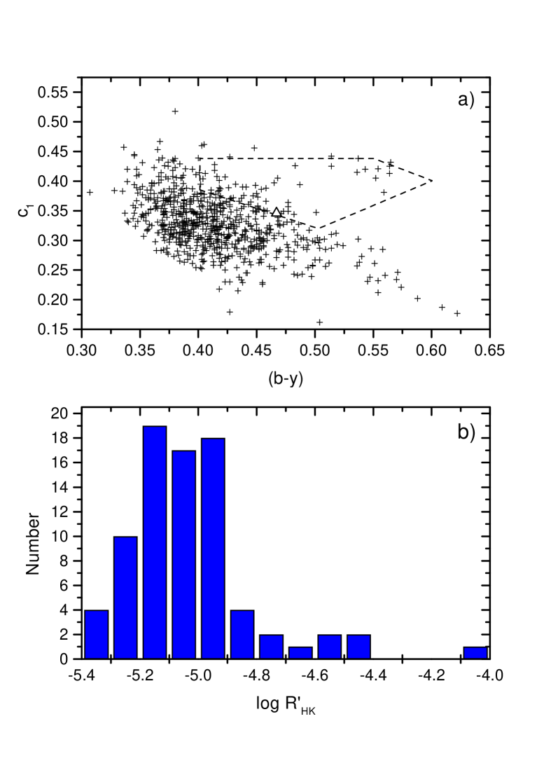
In Figure 1a, the diagram $(b-y)\times c_{1}$ for these 729 stars is shown. The polygon in this figure corresponds to the area of the diagram occupied mostly by subgiants, according to Olsen (olsen84 (1984)). As much as 11% of the sample is probably composed of subgiants. Figure 1b shows a histogram of chromospheric activity levels for these stars. Many of them have $\log R^{\prime}_{\rm HK}<-5.00$, corresponding to a chromospheric age greater than 5.6 Gyr, according to the age calibration by Soderblom et al. (soder91 (1991)), an additional evidence for their evolved status.

One of these supposed subgiants (HD 119022, shown in Figure 1a as an open triangle) is a VAS ($\log R^{\prime}_{\rm HK}=-4.03$), and presumably should be a very young star, not a subgiant. Note that the star is quite near the limit of the subgiant area, and could rather be considered a slightly evolved dwarf. Its nature is still uncertain, since it is located far beyond the zero-age main sequence. Soderblom et al. (SKH (1998)) have studied this star in more detail, and have found spectral features typical of youth (strong Li and broad-line spectrum), but its high luminosity prevented them from classifying it unambiguously as a young star. Other trends in its spectrum (strong H$\alpha$ in absorption, a discrepancy between colour and spectral type, and deep sharp features inside the Na D profiles) suggest that it could be a heavily reddened star. We will return to this star later, and show that the reddening does affect it substantially.

Figure 1: Photometric and chromospheric data for the initial sample of 729 late-type dwarfs. a) Diagram $(b-y)\times c_{1}$ for the initial sample. The polygon indicates the area populated by subgiants, and the open triangle shows the position of the star HD 119022 in this diagram (see text). b) Distribution of chromospheric activity indices of the stars located in the subgiants area.

These ‘subgiant’ stars are probably a mix of thick disk and old thin disk stars. We choose to keep all of them in the initial sample since their number is relatively small and because they most probably represent the older epochs of the disk evolution we are trying to recover. However, it is not presently known whether their chromospheric properties can be related to that of main-sequence stars. At least, as will be demonstrated in the next pages, there is good agreement between their isochrone ages and chromospheric ages.

2.2 Metallicities and colour indices

The calibrations of Schuster & Nissen (schuniss (1989)) were used for the determination of the metallicity of each star. The metallicities for 3 stars redder than $(b-y)=0.599$ were given by the calibration of Olsen (olsen84 (1984)) for K2-M2 stars. To obtain the colours $\delta m_{1}$ and $\delta c_{1}$, we have adopted the standard curves $(b-y)\times m_{1}$ and $(b-y)\times c_{1}$ given by Crawford (crau (1975)) for late F and G0 dwarfs, and by Olsen (olsen84 (1984)) for mid and late G dwarfs. The error in the metallicity from these calibrations is expected to be around 0.16 dex (Schuster & Nissen schuniss (1989)).

To account for the $m_{1}$ deficiency in active stars (Giménez et al. gimenez (1991), and references therein), the photometric metallicity of the active and very active stars ($\log R^{\prime}_{\rm HK}\geq-4.75$) needs to be corrected by adding to it an amount $\Delta{\rm[Fe/H]}$, given by the equation proposed by Rocha-Pinto & Maciel (RPM98 (1998)):

$$\Delta{\rm[Fe/H]}=2.613+0.550\log R^{\prime}_{\rm HK}.$$ (1)

Since this correction is still rather uncertain, we will always present the uncorrected metallicity (which is the quantity that comes directly from the photometric data) in all plots, tables and references in the text, except when mentioned otherwise.

2.3 Chromospheric ages

Chromospheric ages were calculated using the age calibration developed by Soderblom et al. (soder91 (1991); their Equation 3). Besides this calibration, we have tested the calibration by Donahue (1993, as quoted by HSDB). This last calibration gives ages very similar to those of Soderblom et al. (soder91 (1991)), except for stars with $\log R^{\prime}_{\rm HK}>-4.40$, for which it predicts ages systematically lower. We have not used it in our final results for the sake of consistency, as some corrections applied to the chromospheric ages were based on the calibration by Soderblom et al. (soder91 (1991)). Moreover, only 6% of the sample stars have $\log R^{\prime}_{\rm HK}>-4.40$. We have also verified that our conclusions are not dependent on the difference between these age calibrations.

Figure 2: Comparison between chromospheric age calibrations in the literature. Solid line, Soderblom et al. (soder91 (1991), equation 3); circles, Soderblom et al. (soder91 (1991), equation 1); stars, Donahue (don (1993)); dashed line, adopted calibration for three metallicities, namely $-1.2$, $-0.23$ and $+0.4$.

Figure 3: Age distribution for the initial sample. Stars with chromospheric ages greater than 15 Gyr are not shown in this plot.

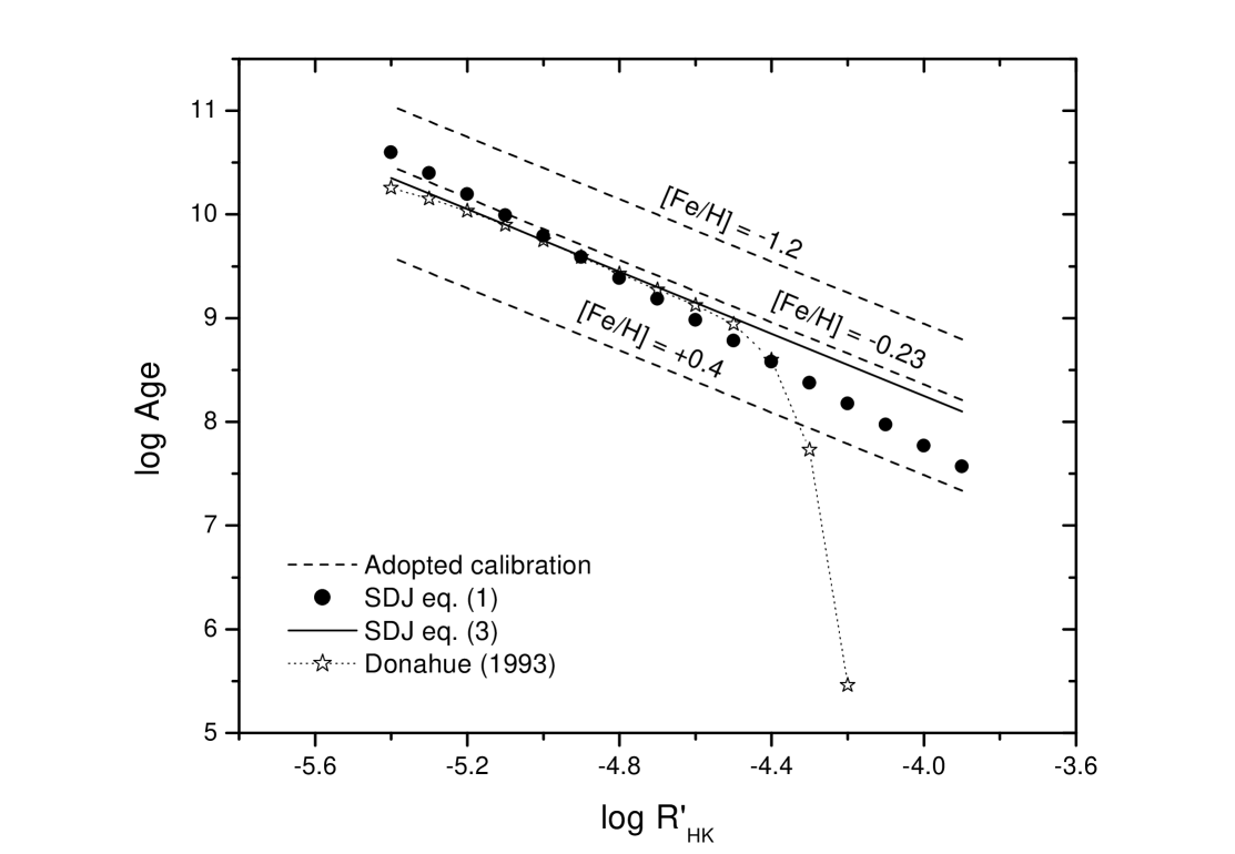
The adopted age calibration was further corrected for the dependence on the metallicity proposed by Rocha-Pinto & Maciel (RPM98 (1998)). In Figure 2, we show a comparison between the uncorrected age calibration, and the same curve corrected for three values of [Fe/H], namely $-1.2$, $-0.23$ and $+0.4$, which corresponds to the lowest, the average and the highest metallicity of our sample. Also presented in the same plot are the age calibrations by Soderblom et al. (soder91 (1991); their Equation 1) and that by Donahue. Most important in this plot is that it shows that the majority of our stars will have an age not very different from that given by the uncorrected Soderblom et al. (soder91 (1991))’s age calibration. This can be seen from the close agreement between the uncorrected age calibration and that for the average metallicity of the sample.

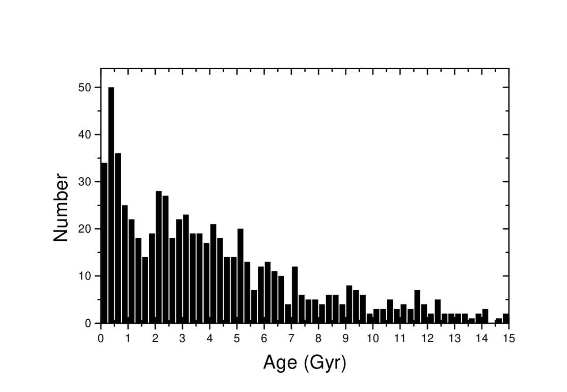
Figure 3 shows the resulting age distribution for all these stars, excluding 54 stars that present ages greater than 15 Gyr. The unrealistically high age of these 54 stars could be caused by one of these reasons: (i) the star is experiencing a Maunder-minimum phase (see Baliunas et al. baliunas (1995)); (ii) the errors in the chromospheric index and in [Fe/H] worked together to produce a spuriosly high age; and (iii) the age calibration could be overestimated for large $\log R^{\prime}_{\rm HK}$ values, since at that range it is given by an extrapolation of data for younger stars.

Figure 4: Error in the index $\log R^{\prime}_{\rm HK}$ due to the stellar magnetic cycles, calculated from the data for 85 stars published by Duncan et al. (duncan (1991)). A small trend is seen in the sense to find the greatest errors in the old redder dwarfs, but the behaviour is not so well defined to allow the use of a formalism describing it. The Sun is also shown in this diagram, in the bottom-left panel.

Several errors contribute to the error in age, coming from the procedures of corrections and transformation of indices into age. We consider two error sources, namely the error in the index $\log R^{\prime}_{\rm HK}$ and the error in the photometric metallicity which enters in the metallicity-dependent correction. Rigorously speaking we should also consider the error in Soderblom et al. (soder91 (1991))’s calibration and the error in the metallicity correction itself. However, these are not independent from the former, since the scatter in the calibration reflects mainly the neglecting of the metallicity correction, as well as the uncertainty in the index.

The average error in $\log R^{\prime}_{\rm HK}$ was estimated from the data published by Duncan et al. (duncan (1991)). They present data for the variation of the $S$ index in several late-type stars, for a time interval of 17 years. We have calculated the corresponding values for $\log R^{\prime}_{\rm HK}$ using the equations by Noyes et al. (noyes (1984)). The index shows much variation for some stars, but the average error is around $\pm 0.05$. This error estimate agrees closely with that made by S85. The uncertainty introduced in the age by the photometric metallicity was estimated by propagating the error in [Fe/H], using the metallicity-corrected age calibration given by Rocha-Pinto & Maciel (1998).

A further complication arises if we consider other error sources: flaring, rotational modulation of active regions, and the stellar magnetic cycles. A small part of this error is already incorporated into the error in $\log R^{\prime}_{\rm HK}$, but some stars show much variation in the chromospheric indices. Donahue (don98 (1998)) shows that the age of the Sun could be miscalculated within an error of several Gyr if its chromospheric age were derived from observations in an epoch of maximum or minimum activity. S85 remarks that the most serious problem is with the stellar magnetic cycles, and the effects of the other sources of variability are smaller. This uncertainty is the major problem of the chromospheric ages. It can be much decreased provided that we have a good determination of the mean stellar activity, which is still not the case for the majority of the stars in the solar neighbourhood. The promising accuracy of this technique was presented also by Donahue (don98 (1998)), who has shown that the age discrepancy between binaries is usually lower than 0.5 Gyr for systems younger than 2 Gyr, and does not exceed 1.0 Gyr for older pairs.

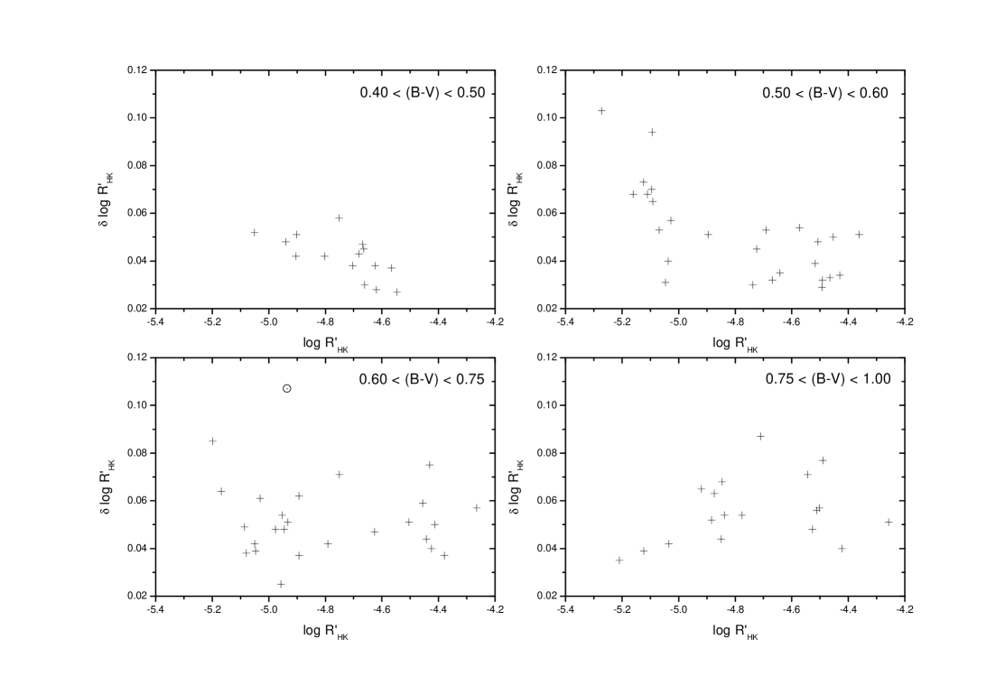
We have investigated this error with more detail in the data published by Duncan et al. (duncan (1991)), for 85 stars that have been continuously monitored from 1966 to 1983. The $\log R^{\prime}_{\rm HK}$ index for each of these stars was calculated, and an average error was found. The results are presented in Figure 4, where we have separated the stars according to their colours. The Sun is also shown in this diagram (in the bottom-left panel). To calculate its position, we have used the $S$ indices for the maximum and minimum activity during cycles 20-22, given by Donahue (don98 (1998)).

Note that there is a small tendency to find the biggest errors in the redder stars. This pattern follows more or less closely the findings by Baliunas et al. (baliunas (1995)), who have shown that F dwarfs do not show much magnetic variability, while the redder dwarfs present very well defined magnetic cycles. This can increase the error in $\log R^{\prime}_{\rm HK}$ beyond the value we have adopted, since from only one observation it is impossible to know exactly in what part of the cycle the star is. On the other hand, it is evident from the figure that no single law can be used to estimate the error in the index, given the chromospheric activity level and the stellar colour.

The $\log R^{\prime}_{\rm HK}$ error for the Sun is one of the greatest. It is not clear yet whether it is caused by our more accurate knowledge of the solar magnetic activity (for instance, the time span for the solar $S$ measurements in this figure is about 3 times longer than that of the stars), or to a real more pronounced magnetic variability in the Sun.

Around 80% of our sample is composed of stars having only one $\log R^{\prime}_{\rm HK}$ measure. Their ages are most subject to the errors due to stellar magnetic cycles. Nevertheless, the incorporation of this kind of error is very difficult, and we have decided to use a conservative value of 0.05 dex calculated as described above. This error is 0.01 dex greater than that estimated by S85 for 33 dwarfs. According to this author, on the average the star will present an uncertainty around 10% in $\log R^{\prime}_{\rm HK}$ (0.04 dex), due to the stellar magnetic cycles. This procedure will not affect significantly our conclusions, since the error in $\log R^{\prime}_{\rm HK}$ is small compared to that due to the photometric metallicity.

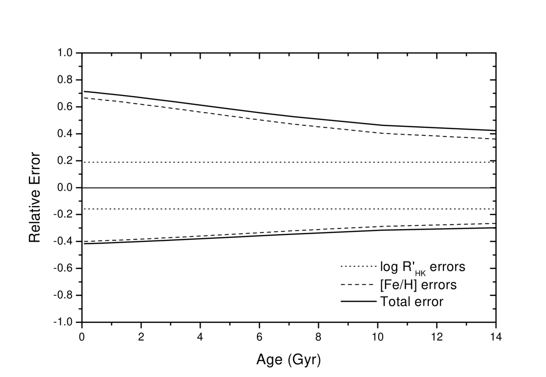
The impact of the individual error sources on the age is shown in Figure 5, which shows relative errors ($\varepsilon_{\rm age}/{\rm age}$), as a function of age. The final error in age, shown as a solid line, was calculated by adding those two individual errors in quadrature. This is the error estimate used throughout this paper. As can be seen from the error trends in the plot, the positive error in the age is greater than the negative error. This is due to the logarithmic nature of the age calibration and the metallicity corrections. We expect that many stars will show ages scattered over a large range of values above the real stellar age. This is one of the reasons why some stars present unreasonable ages greater than 15 Gyr.

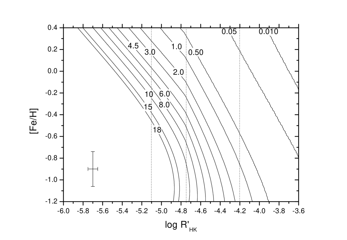
Since the chromospheric age depends not only on the activity level of the star but also on its metallicity, the task of finding a chromospheric age is analogous to find an ‘isochrone’ age in the metallicity–activity diagram, as shown in Figure 6. This figure shows lines of equal chromospheric age, expressed in Gyr. The dotted vertical lines are used to separate the four chromospheric populations, as defined section 2.1. An interesting result is that while for G dwarfs the younger isochrones are crowded in the colour–magnitude diagram, preventing one from obtaining accurate isochrone ages for very young stars, they are much more spaced in the metallicity–activity diagram. The opposite occurs for the older isochrones being more crowded in this last diagram. From this we can see that chromospheric ages are most useful for younger stars, losing part of their accuracy as we consider older stars.

Figure 5: Relative errors in the chromospheric ages. The curves show the individual contribution of each error sources to the error in age. The curves stand for the error in the index $\log R^{\prime}_{\rm HK}$ (dotted lines), and in the photometric metallicity (dashed lines). The final age error was calculated by the root mean square of all these errors and is shown as thick solid lines.

Figure 6: Curves of equal chromospheric age in the metallicity–activity diagram. The average error in this diagram is shown at the lower left corner. The vertical dotted lines separate the four groups of stellar activity, as defined in section 2.

Figure 7: Histogram of distances from the Sun, for the initial sample. The majority of the stars are located within 60 pc, but 5% of them have distances greater than 100 pc.

2.4 Parallaxes, absolute magnitudes and reddening

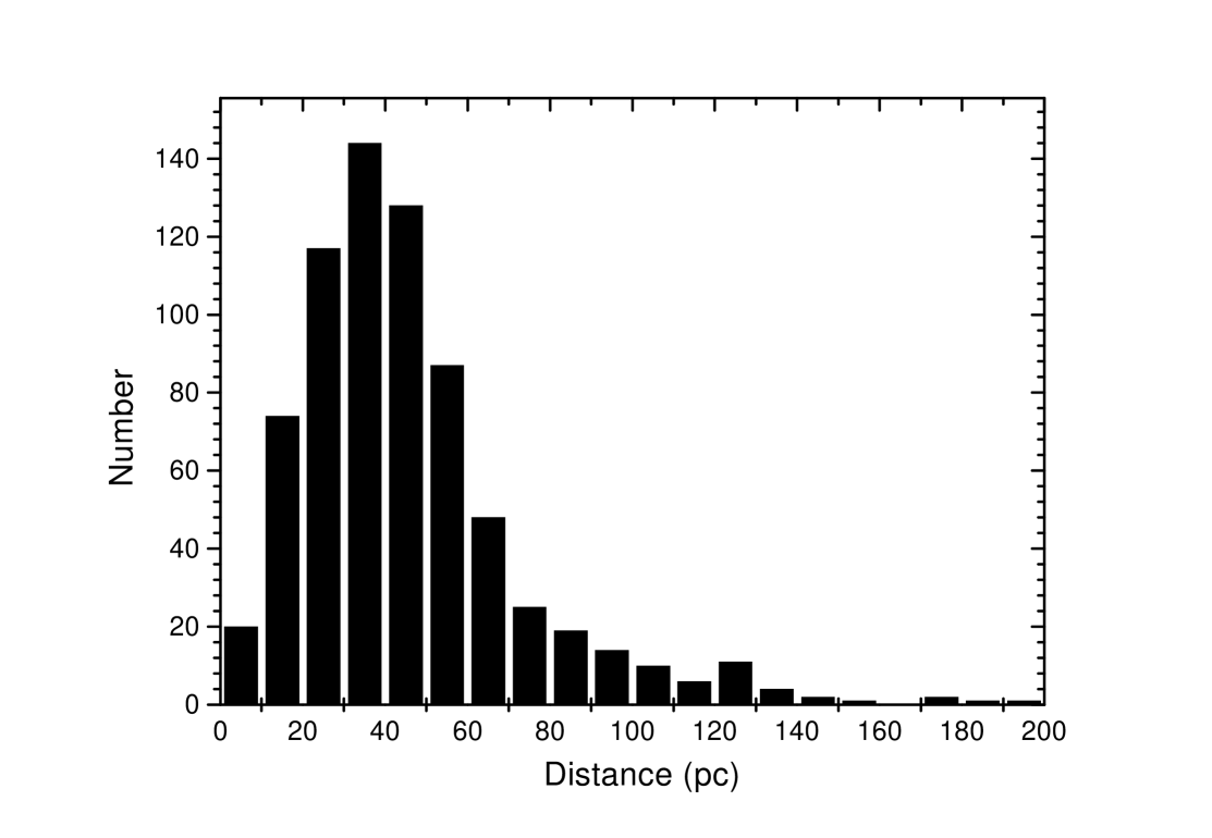
Parallaxes and absolute magnitudes were obtained from the HIPPARCOS data for 714 of these stars. The histogram in Figure 7 shows the distribution of distances of the stars from the Sun. The majority of the stars are located within 60 pc, but 5% of them have distances greater than 100 pc.

We have calculated the reddening for 13 of these stars located beyond 100 pc, using $\beta$ indices from Hauck & Mermilliod (HM98 (1998)) and the intrinsic colour calibration of Schuster & Nissen (schuniss (1989)). The results are presented in Table 1 where we list the HD number, the distance from the Sun, $\log R^{\prime}_{\rm HK}$, the colour excess $E(b-y)$, the dereddened Strömgren indices $(b-y)_{0}$, $m_{0}$ and $c_{0}$, the photometric metallicity calculated with the dereddened indices, and the difference between the previous [Fe/H] calculated without and with reddening correction. Four of these stars present $E(b-y)<0$ and should not be reddened. Thus, dereddened indices are not provided for them in the Table.

The Table shows that there is considerable reddening for some stars, and this can seriously affect the stellar metallicity. Provided that we had $\beta$ for all the stars located beyond 100 pc, we could deredden their indices and find more reliable estimates for [Fe/H], and consequently age, but this index is available only for a few stars. To avoid reddened stars, in the next sections we will consider generally only those stars located within 80 pc, for which reddening is expected to be negligible (Olsen olsen84 (1984)).

Note that the reddening for HD 119022 is appreciable, confirming the suggestion by Soderblom et al. (SKH (1998)). Moreover, taking the dereddened colours in Table 1, we see that the star resides outside the subgiant polygon in Figure 1a, right in the bulk of main-sequence stars. This can be taken as additional evidence for a lower age.

Table 1: Data for 13 reddened stars in the sample.

Name	$d({\rm pc})$	$\log R^{\prime}_{\rm HK}$	$E(b-y)$	$(b-y)_{0}$	$m_{0}$	$c_{0}$	${\rm[Fe/H]}_{\rm dered}$	$\Delta{\rm[Fe/H]}$
HD 3611	$104.6$	$-5.150$	$0.014$	$0.374$	$0.166$	$0.404$	$-0.386$	$-0.030$
HD 17169	$107.9$	$-4.720$	$0.040$	$0.432$	$0.231$	$0.332$	$-0.044$	$-0.300$
HD 39917	$194.9$	$-4.050$	$0.064$	$0.454$	$0.254$	$0.298$	$-0.180$	$-0.444$
HD 119022	$124.2$	$-4.030$	$0.054$	$0.420$	$0.231$	$0.336$	$+0.053$	$-0.397$
HD 122683	$176.7$	$-4.760$	$-0.018$
HD 139503	$109.9$	$-5.180$	$0.017$	$0.376$	$0.182$	$0.385$	$-0.057$	$-0.144$
HD 141885	$104.1$	$-5.340$	$0.019$	$0.390$	$0.208$	$0.459$	$+0.155$	$-0.160$
HD 142137	$105.8$	$-5.040$	$0.024$	$0.381$	$0.194$	$0.435$	$+0.059$	$-0.210$
HD 151928	$114.8$	$-5.070$	$-0.023$
HD 159784	$124.8$	$-5.200$	$-0.032$
HD 179814	$133.3$	$-4.970$	$-0.017$
HD 199017	$173.6$	$-4.920$	$0.026$	$0.412$	$0.213$	$0.325$	$-0.072$	$-0.195$
HD 202707	$112.0$	$-5.110$	$0.027$	$0.396$	$0.185$	$0.343$	$-0.188$	$-0.225$

Five objects amongst the 13 VAS of our sample have distances greater than 100 pc. We expect that they are mildly to strongly reddened. The straightforward consequence of this is that their photometric metallicities would seem lower than they really are. This can be seen from Table 1 where there are two VAS listed: HD 39917 and HD 119022, with a metallicity difference of around $-0.4$ dex. Rocha-Pinto & Maciel (RPM98 (1998)) showed that the photometric metallicity distribution of the VAS is peculiarly concentrated at lower [Fe/H], in strong contrast with the expected youth of such stars. We have explained this trend as the result of the $m_{1}$ deficiency, which makes stars with strong chromospheres resemble metal-poor stars from a photometric point of view. This deficiency can originate from the filling in of the line cores due to a chromosphere-driven photospheric activity (Basri, Wilcots & Stout basri (1989)).

However, these new results suggest that the low photometric metallicities of the VAS could be explained as an effect of the reddening. At least, the difference in the metallicity, $\Delta{\rm[Fe/H]}$, is large enough to make the photometric metallicity of the VAS very similar to the metallicity of the AS, in the ${\rm[Fe/H]}\times\log R^{\prime}_{\rm HK}$ diagram. We need to know if the reddening can explain the ‘activity strip’ found in this diagram (Rocha-Pinto & Maciel RPM98 (1998)), since our procedure to correct [Fe/H] in the AS and VAS, for the effects of the $m_{1}$ deficiency, depends on the meaning of this strip.

Only one other VAS has a published $\beta$ in the literature. It is HD 123732 which shows a very small reddening, $E(b-y)=0.002$, in agreement with its distance from the Sun (around 63 pc). However, its photometric metallicity is not very low (${\rm[Fe/H]}=-0.220$) compared to other VAS. If we were to trust its youth, we would need to explain its subsolar [Fe/H] as an evidence towards the $m_{1}$ deficiency. Notwithstanding, Soderblom et al. (SKH (1998)) have found features in its spectrum that classify it as a W UMa star, so that its chromospheric activity must not come from youth. On the other hand, Soderblom et al. measured spectroscopic [Fe/H] in two VAS which are most probably very young single stars, and the difference between these metallicities and the photometric metallicities are in very good agreement with our prediction in Equation (1). Both are located within 50 pc, and therefore are unreddened. The difference between the spectroscopic and photometric [Fe/H] can only be understood as resulting from the $m_{1}$ deficiency.

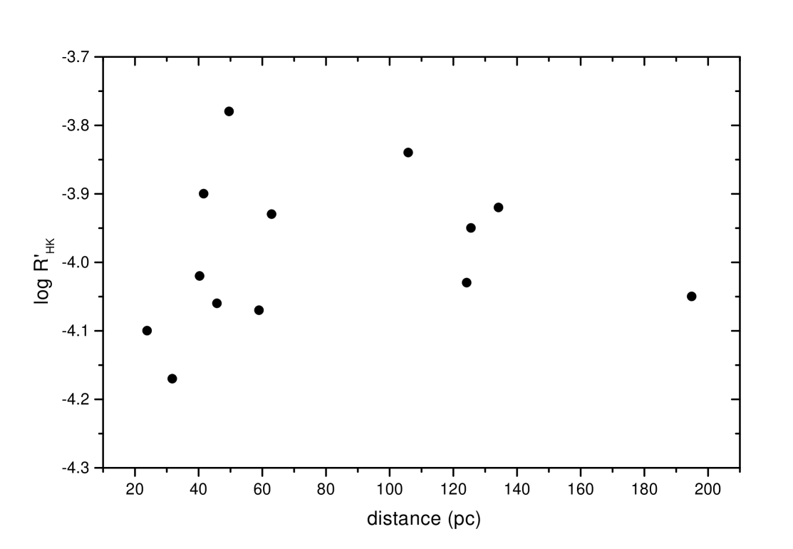
It is important to bear in mind that what Rocha-Pinto & Maciel (RPM98 (1998)) have found seems to be a systematic trend depending on $\log R^{\prime}_{\rm HK}$: the more active the star is, the more metal-deficient it looks. This trend makes the $m_{1}$ deficiency hypothesis very appealing, since it can produce a similar effect. If this behaviour is likely to be produced instead by reddening, then we need to consider a correlation between distance and $\log R^{\prime}_{\rm HK}$. Figure 8 shows that such a correlation probably does not exist. The most distant VAS are not the most active. In fact, even disregarding the most distant VAS, the ${\rm[Fe/H]}\times\log R^{\prime}_{\rm HK}$ diagram still presents the ‘activity strip’. The average metallicity of the VAS within and beyond 80 pc (our chosen distance cutoff) is $-0.318$ and $-0.480$ dex, respectively, showing that while reddening can explain part of the low photometric metal-content of the VAS, there is still another effect to account for, and the $m_{1}$ deficiency seems the most promising one.

Since the proposed correction for the $m_{1}$ deficiency was empirically determined using only AS stars, and they do not seem to be affected by reddening, we have no reason to disregard them. Indeed, the agreement of our proposed correction with the two VAS studied by Soderblom et al. (SKH (1998)) is good evidence that the extrapolation of the relation for the VAS is reasonable.

Figure 8: Activity level versus distance from the Sun, for the VAS. The plot shows that a correlation between these quantities probably does not exist. The most distant VAS are not the most active. While reddening can explain part of the low photometric metal-content of some VAS, there is still another effect to account for, and the $m_{1}$ deficiency seems the most promising one.

2.5 Effects of unresolved binarity

According to Duquennoy & Mayor (mayor (1991)), 65% of the G dwarfs in the solar neighbourhood are presently unresolved binaries. They are expected to present colours contaminated by the unresolved secondary, which would introduce errors in their metallicities and ages. We are here primarily concerned in the age errors, that can be more easily estimated. Since there is no set of chromospheric measurements for combined and resolved binaries, this discussion is predominantly theoretical.

Figure 9: Expected number of binaries in each age bin, shown by dark bars. The dashed line shows the total number of stars in each bin. The solid line indicates the expected relative age error of the unresolved stars, as a function of age. The error is always positive, since unresolved stars appear younger than they really are.

In principle, for two stars with the same age and metallicity, $\log R^{\prime}_{\rm HK}$ are equal. The index that depends on the colour is the $S$ index. For two coeval stars, born from the same parental cloud, $S$ will be greater in the cooler one. The index is very dependent on the stellar colour, since the chromospheric flux is much greater in the late type stars. When two stars are observed as one star, the $S$ index of the primary will be contaminated by that of the secondary. The combined index will be always greater than that of the primary, and the star would appear more active and younger than it really is.

We have calculated the $S$ index that would correspond to a certain $\log R^{\prime}_{\rm HK}$ for several binary pairs, with $(B-V)$ varying from 0.4 to 1.0, by inverting the equations provided by Noyes et al. (noyes (1984)). A larger colour range could not be used due to the limit of the $S$ calibration to colours higher than $(B-V)=1.0$. The $(B-V)$ colour was also used to estimate roughly the effective temperature and mass of the star. We thus can calculate the mass ratio for each pair (secondary to primary).

To combine the $S$ index of the two stars in the pair, we used a weighted mean. The weight is the Planck function integrated from $\lambda\lambda$ 3880 to 4020 Å, which correspond to the spectral range where the Ca II lines are found. In this way, we can found an average $S$ for the unresolved pair, and the corresponding $\log R^{\prime}_{\rm HK}$. We compared the difference between this average $\log R^{\prime}_{\rm HK}$ and the real index, known a priori. Basically, the difference is greater for the active stars, since the $S$ index of the secondary becomes much greater than that of the primary. For the inactive stars, it is lower than 0.04 dex which is smaller than the error for the index presented in Figure 5. The difference depends also on the mass ratio, and on the primary mass. A larger mass ratio tends to increase the difference. That means that a pair of stars composed of a G+K dwarf will appear more active than that composed by two G dwarfs. But at a certain mass ratio, around 0.55, the behaviour changes and the difference diminishes. That is, a pair composed of a G+M dwarf would be much less contaminated than that composed of a G+K dwarf. This reflects the fact that the intensity of the spectrum of the hotter star becomes much more important than that of the fainter. The dependence on the primary mass is simpler: the more massive is the primary, the weaker is the contamination by the secondary, and the smaller is the difference in $\log R^{\prime}_{\rm HK}$.

Since these are just rough estimates, we decided to keep the qualitative approach, instead of deriving numerical corrections. We have calculated the number of stars in each age bin that can have a wrong age due to unresolved binaries. This number is estimated as

$$N_{\rm b}=\Delta Nf_{\rm bin}f_{{m_{<1.2}}}f_{q},$$ (2)

where $\Delta N$ is the number of stars in each age bin; $f_{\rm bin}$ is the fraction of unresolved binaries in the sample, taken as 0.65; $f_{{m_{<1.2}}}$ is the fraction of stars with masses lower than $1.2M_{\odot}$, which are expected to be much influenced to contamination by a secondary, according to our calculations; and $f_{q}$ is the percentage of mass ratios in which the primary $S$ colour are affected by that of the secondary. From a Salpeter IMF, we estimate that $f_{{m_{<1.2}}}\approx 0.67$. The fraction $f_{q}$ is conservatively estimated as 0.50 from our calculations. In this last estimate entered the fact that two stars with mass ratio around 1 will not affect the results: they would have the same index; and stars much fainter will not contaminate the index of the primary.

Figure 10: Comparison between the main characteristics of the initial (729 stars) and the additional samples (267 stars). These main characteristics are the metallicity distribution (upper-left panel), chromospheric activity distribution (upper-right panel), and the metallicity–activity distribution (bottom panels).

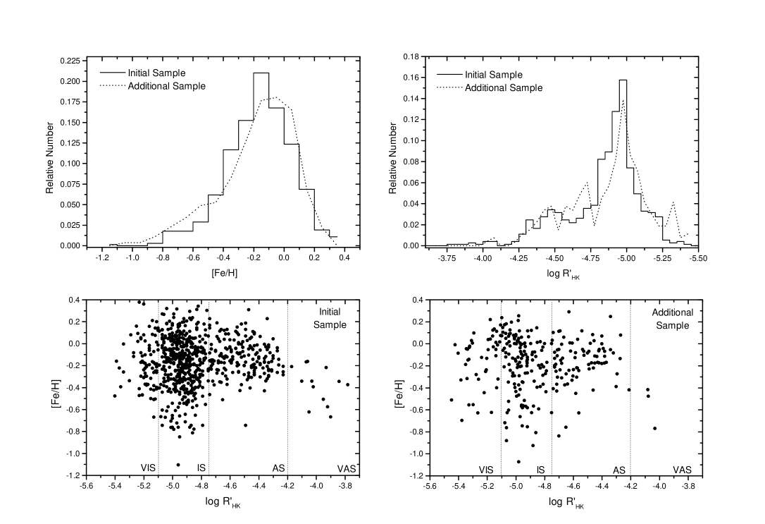
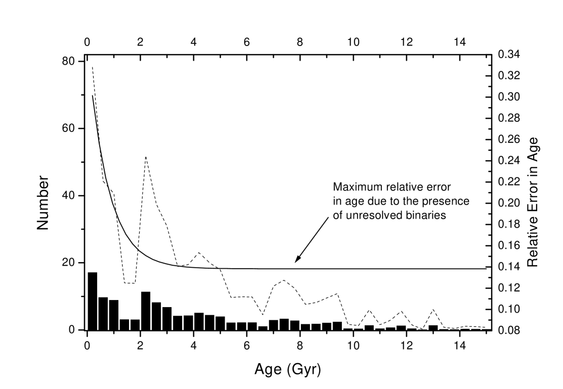
Figure 9 shows the number of stars with probably wrong ages due to duplicity. The solid line in this plot gives the expected relative age error for those stars. It uses the maximum error in $\log R^{\prime}_{\rm HK}$, after varying the primary mass and the mass ratio. The error is always positive, since unresolved stars appear younger than they really are.

It can be seen that the error is greater for the youngest stars. However, its magnitude is negligible in view of the age errors already considered in Figure 5. The number of stars subject to this errors is also small, so that we can conclude that it does not affect the main results of this paper.

2.6 Representativeness of the sample

An additional sample, consisting of 267 stars, was built in order to complement our initial sample. The sample consists of stars initially in the surveys of S85 and HSDB, but not having photometric data in Olsen’s catalogues, as well as other stars scattered amongst several papers by the Mount Wilson group (Soderblom et al. soder91 (1991); Duncan et al. duncan (1991); Baliunas et al. baliunas (1995); Saar & Donahue saar (1997)), including the Sun itself which has not entered in the initial sample. In some cases, only the $\langle S\rangle$ index was provided, and we calculated the corresponding $\log R^{\prime}_{\rm HK}$ indices using the formalism of Noyes et al. (noyes (1984)). Photometric data for these stars were taken from the catalogue of Hauck & Mermilliod (HM98 (1998)).

In figure 10 we show the main characteristics of both the initial and the additional sample: the metallicity and $\log R^{\prime}_{\rm HK}$ distributions and the metallicity–activity diagram. In all three aspects considered, both samples differ somewhat. The metallicity distribution of the additional sample is broader, and the metallicity–activity diagram seems more scattered than that for the initial sample. Part of this scatter probably reflects the heterogeneity of the photometric data in the catalogue of Hauck & Mermilliod (HM98 (1998)). Moreover, there are also significant differences between the chromospheric activity distribution of the two samples. One of these differences is the excess of stars with $-4.75<\log R^{\prime}_{\rm HK}<-4.60$, where the Vaughan-Preston gap is supposed to be located. Far from being evidence for the non existence of this feature, this excess must be understood as a bias, due to the preferential publication of data for objects with certain activity levels, since they were gathered from scattered papers of the Mount Wilson group aimed at the study of small samples built from different selection criteria. Thus, we cannot join the two samples since the representativeness would be lost. This problem is very important to our study as long as our ultimate goal is counting stars with certain activity levels, after having converted them to ages, to find the star formation history (see Paper II). Since the photometric and chromospheric data come from heterogeneous sources, we decided to use this sample only as an additional tool for our study, in those topics where its inclusion is not likely to change the representativeness of the sample.

Figure 11: Comparison between the chromospheric activity distributions for the S85 and HSDB surveys.

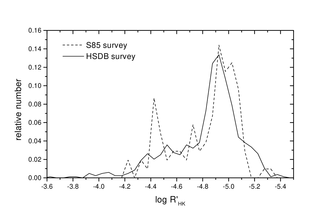
In practice, we have to ask whether the initial sample itself is representative since to the present moment the $\log R^{\prime}_{\rm HK}$ indices for many stars observed by the Mount Wilson group have not been published. We can only base our suppositions about the shape of the stellar chromospheric activity distribution on the two surveys already published: S85 and HSDB. The first of these surveys includes data for 177 nearby stars in the northern hemisphere, while HSDB gives data for 817 southern hemisphere stars. In Figure 11, we have compared the activity distribution of both surveys. Inspection of this plot shows that the agreement between these distributions is only fair. It is possible to see a separation between active and inactive stars in both surveys, but the relative number of stars in the activity levels seems to be different in them.

The HSDB survey has selected stars from the combination of the two-dimensional MK spectral types in the surveys by Houk and collaborators (Houk & Cowley HC (1975); Houk houk78 (1978); Houk houk82 (1982); Houk & Smith-Moore HSM (1988)) with the photometric data by Olsen (olsen88 (1988), olsen93 (1993)). A secondary sample composed by 119 stars, not present in Olsen’s papers was also observed by them to compensate for the incompleteness of these (see below).

Houk’s surveys includes all stars in the Henry Draper Catalogue, from which Olsen also has constructed his database for photometric observations. The Henry Draper Catalogue is supposed to be nearly complete to magnitude $V<9$, but Olsen’s catalogue has some biases towards more massive stars, as explained in Olsen (olsen93 (1993)). However, these biases are not expected to depend upon any age-related quantity. Thus, the only biases expected for our southern hemisphere stars are those present in Olsen’s catalogues. The limiting magnitude for completeness is $V=8.3$ mag, which is the brighter cutoff present in Olsen’s catalogues (Olsen olsen83 (1983)). For northern hemisphere stars, the sample is based upon the Catalogue of stars within Twenty-five Parsecs of the Sun (Wooley et al. wooley (1970)), which also constitutes a complete sample of nearby solar-like stars.

We are inclined to assume that the HSDB survey best represents the real galactic chromospheric activity distribution, since it includes the largest sample. A comparison between the primary and secondary sample in the HSDB survey (see their Figure 5), for example, shows that the secondary sample (119 stars) present a broader chromospheric acticity distribution between $-4.80<\log R^{\prime}_{\rm HK}<-5.10$, agreeing more with the the S85 survey. However, a definitive answer to this question can only be given when data for a sample of northern hemisphere stars, as extensive as that of HSDB, is published.

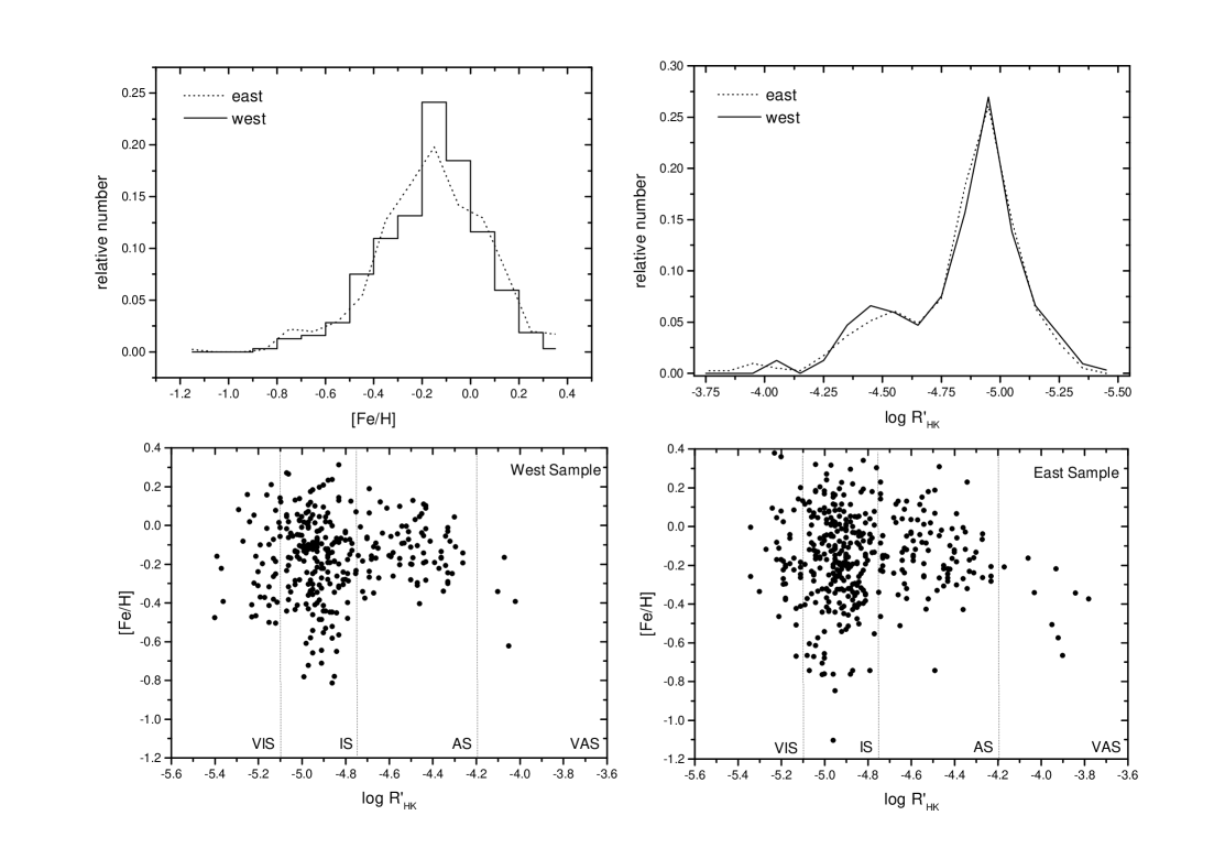
Around 87% of our sample is composed of southern hemisphere stars, and this makes our chromospheric activity distribution very similar to that of the HSDB survey. But this does not warrant the representativeness of ours, since we would be comparing very similar samples. At least, we can look for some biases if we divide our sample and verify whether both subsamples keep the same characteristics. We have done this by separating the stars according to right ascension: stars with R.A. from 0$\aas@@fstack{h}$ to 12$\aas@@fstack{h}$ compose the west sample (410 stars), while that with R.A. greater than 12$\aas@@fstack{h}$ compose the east sample (319 stars). In Figure 12 we show the metallicity and $\log R^{\prime}_{\rm HK}$ distributions and the metallicity–activity diagram for the west and east subsamples. Note that the agreement between them is much better in all three characteristics we have considered. According to this, we can assume that probably there is a representative disk chromospheric activity distribution.

Figure 12: Comparison between the main characteristics of the west (R.A $<12\aas@@fstack{h}$) and east (R.A $>12\aas@@fstack{h}$) subsamples. The panels show the same diagrams as in Figure 10.

2.7 Spatial Velocities and Orbital Parameters

For 460 stars from the initial and the additional sample, a radial velocity measurement was found in the literature. These stars compose the ‘kinematical sample’. Each star had its spatial velocities ($U$, $V$ and $W$) calculated from the data in the literature, using the equations provided by Johnson & Soderblom (JS (1987)). Their orbits were then determined by numerical integration within a model of the Galactic potential, for the calculations of the peri- and apo-Galactic distances, $R_{p}$ and $R_{a}$ and the mean Galactocentric radius, $R_{m}=(R_{p}+R_{a})/2$ for the orbit (cf. Edv93), eccentricity and height above the galactic plane.

The kinematical sample is particularly used in a future paper of this series aimed to the study of kinematical constraints related to age. Details on this subsample is to be given in that papers.

3 The chromospheric age–metallicity relation

For the derivation of the age–metallicity relation, we have to correct the metallicity of the AS and VAS for the $m_{1}$ deficiency. Figure 13 shows the age–metallicity diagram for the whole initial sample, up to 15 Gyr. The stars seem to fall along a very smooth relation just like what is expected from chemical evolution theory: the rich stars are the youngest, and the poor ones are the oldest. A surprising result is that the scatter is much smaller than that found by Edv93 using isochrone ages. The significance of this will be discussed later.

Figure 13: Age–metallicity diagram of the initial sample (729 stars). The metallicities of the VAS and the AS are corrected for the $m_{1}$ deficiency. Stars with chromospheric ages greater than 15 Gyr are not shown in this plot.

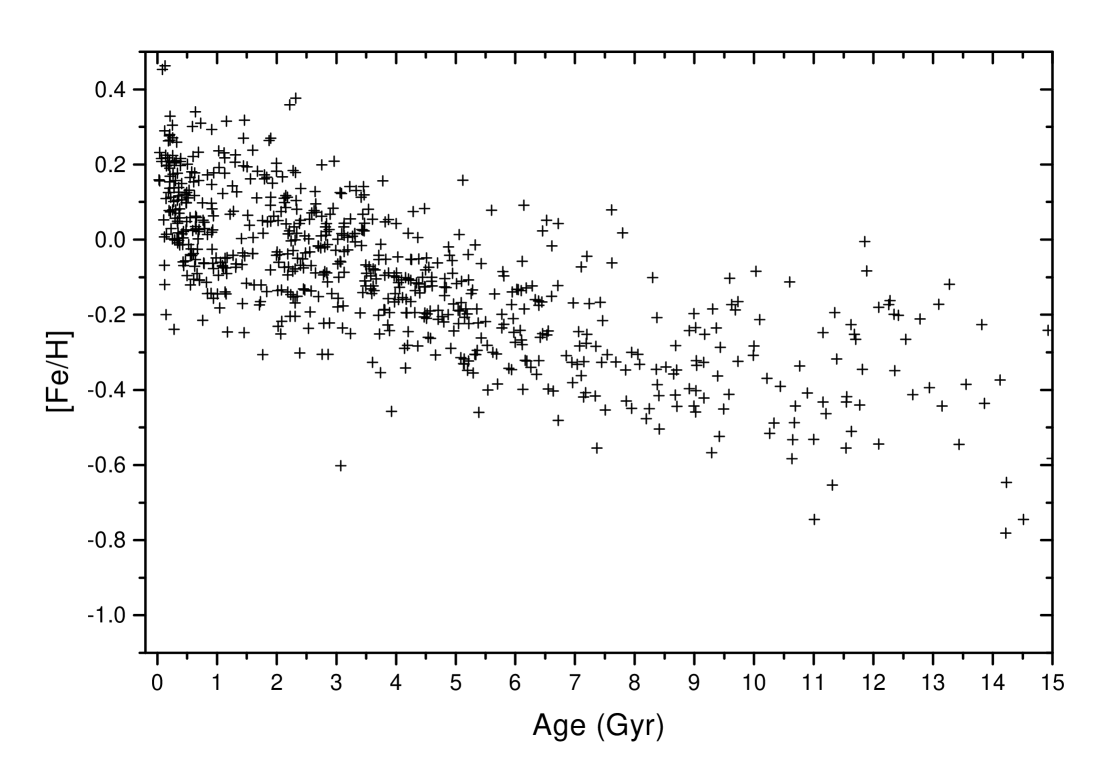
To find a more refined and unbiased AMR, the sample needs further selection. First, we have eliminated 72 stars more distant than 80 pc. Taking into account also 11 stars that do not have parallaxes measured by HIPPARCOS, our sample is reduced to 645 stars. As we want to apply a volume correction to the AMR (Twarog twar (1980)), the sample was further limited to apparent $V$ magnitudes lower than 8.3 mag, by the elimination of 42 stars.

Eight remaining VAS were also eliminated, since many of them may be old close binaries, in which the high activity is produced by highly synchronized rotation, and is not related with age. This can explain why some stars with ages lower than 0.5 Gyr still present subsolar [Fe/H] in Figure 13. Rigorously speaking, one may ask why we have not discarded the VIS since their very low activity might also be unconnected with age and could reflect an evolutionary phase analogous to the Maunder Minimum through which the Sun passed during the 17th-18th centuries (Baliunas et al. baliunas (1995); HSDB). We keep the VIS in our sample as the effects of the metallicity on the $\log R^{\prime}_{\rm HK}$ index make the richer stars resemble older IS, or VIS. Many stars amongst the VIS can be normal stars, and there is presently no way to separate them from the Maunder-mininum stars. The same kind of contamination by normal stars does not significantly affect the VAS group, as can be seen from Figure 6 of Rocha-Pinto & Maciel (RPM98 (1998)).

Seven active stars are known to present greater velocity components (Soderblom soder90 (1990)), and they probably are not young stars (Rocha-Pinto, Castilho & Maciel RPCM (2000)). All of these stars were eliminated from the sample. Finally, disregarding 37 stars older than 15 Gyr, we arrive at a sample with 552 stars. The criteria for elimination are summarized in Table 2.

Table 2: Criteria for eliminating stars of the sample.

Criterion	stars eliminated
Stars not having parallaxes in the HIPPARCOS database	11
Stars distant by more than 80 pc	72
Apparent V magnitude greater than 8.3 mag	42
Very active stars ($\log R^{\prime}_{\rm HK}\geq-4.20$)	8
Objects known to be chromospherically young, but kinematically old	7
Stars with nominal chromospheric ages greater than 15 Gyr	37

3.1 Magnitude-limited AMR

Since our sample is not volume-limited, we have to apply a correction to account for the dependence on [Fe/H] of the apparent magnitudes. This procedure, called volume correction, was already used by some authors (Twarog twar (1980); Ann & Kang annkang (1985); Meusinger et al. meu (1991)). After binning the stars, each metallicity is weighted by $d^{-3}$, where $d$ is the maximum distance at which the star would still have an apparent magnitude lower than the magnitude limit, which for our sample is 8.3 mag. It is given by

$$8.3-M=5\log d-5,$$ (3)

where $M$ is the absolute magnitude of the star.

Table 3: Magnitude-limited AMR.

Age	$N$	$\langle{\rm[Fe/H]}\rangle$	$\sigma_{\rm[Fe/H]}$
0-1	$107$	$+0.12$	$0.13$
1-2	$61$	$+0.01$	$0.14$
2-3	$79$	$-0.08$	$0.12$
3-4	$66$	$-0.10$	$0.12$
4-5	$58$	$-0.15$	$0.08$
5-6	$44$	$-0.26$	$0.11$
6-7	$32$	$-0.28$	$0.13$
7-8	$26$	$-0.33$	$0.14$
8-9	$17$	$-0.36$	$0.10$
9-10	$21$	$-0.39$	$0.12$
10-11	$10$	$-0.40$	$0.14$
11-12	$13$	$(-0.45)$	$0.17$
12-15	$18$	$(-0.48)$	$0.20$

Figure 14: Averaged magnitude-limited AMR (552 stars) compared to previous relations in the literature. The metallicities of the VAS and the AS are corrected for the $m_{1}$ deficiency

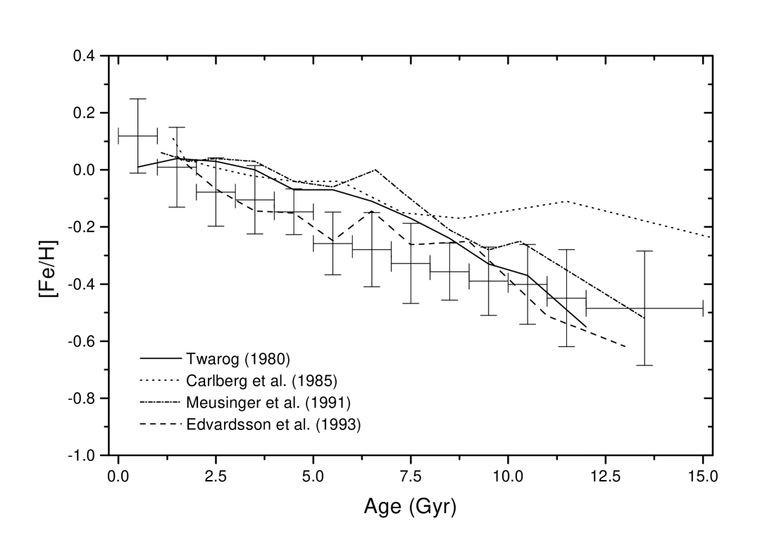
This magnitude-limited AMR is presented in Table 3, where we give the number of stars in each metallicity bin, the average-weighted [Fe/H], corrected for the $m_{1}$ deficiency (see section 2.2), and the metallicity dispersion. The metallicity of the last two bins is presented between parenthesis, since they are expected to be upper limits (see next section). For the calculation of the metallicity dispersion, we have used the same weights, given by Equation (3). These data are presented also in Figure 14, compared with previous relations published in the literature. In spite of having found a somewhat lower metallicity dispersion, we see a good agreement with the mean points of the Edv93’s AMR. The agreement with the AMRs by Twarog (twar (1980)) and Meusinger et al. (meu (1991)) is marginal. These AMRs predict a steady growth of [Fe/H] with time, but with a significant flattening in the last 5 Gyr. Instead, we have found a steepening in the growth of [Fe/H] at that same epoch, a feature also apparent in Edv93. In the oldest age bin, our AMR gives an average metallicity of $-0.48$ dex which is $0.14$ dex higher than the average metallicity in Edv93. We believe that this discrepancy results from the errors in the chromospheric ages (see discussion on section 3.2).

We have not found an absence of metal-rich stars with ages between 3 and 5 Gyr (Carraro et al. carraro (1998)). In fact, our metal-rich stars are very concentrated at the younger bins, since this AMR does not show the large scatter present in other studies.

3.2 The initial metallicity of the disk

The AMR presented in Table 3 indicates a high estimate for the initial metallicity of the disk. According to it, we should expect an average [Fe/H] $\approx-0.48$ dex at around 13.5 Gyr ago. This metallicity is somewhat higher than the corresponding values found by Twarog (twar (1980)) and Edv93.

A high initial metallicity is indicative of significant pre-enrichment of the gas before the formation of the first stars in the disk. That the disk has had some previous enrichment can be easily seen from the lower cuttoff in its metallicity distribution in [Fe/H] $\approx-0.8$ dex (Rocha-Pinto & Maciel RPM96 (1996)). Even in the framework of an infall model, the disk initial metallicity must be non-zero in order to match the G-dwarf problem.

Our AMR has a peculiar behaviour towards greater ages. It flattens while the other relations (as well as the theoretical models) generally becomes steeper, indicating a rapid enrichment in the early galactic phases. That flatenning is the major difference between the mean points of our AMR and the mean points of that by Edv93.

The behaviour of our AMR in the oldest age bins are probably very affected by the age errors discussed in section 2. The chromospheric activity yields more accurate ages for younger stars, and we expect that the AMR at the youngest bins is fairly well reproduced. For the older bins, however, we have to estimate the mean deviation from the real AMR that we expect to find from using chromospheric ages. This can be done by simulating the scattering of the stars in the AMR due to the age errors.

The procedure follows closely that used in Paper II to compute the statistical confidence levels for the star formation history (hereafter SFH) features, and we refer to that paper for more detail. We simulate a constant SFH composed by 3000 stars. For each star, a metallicity is assigned by a pre-adopted AMR. After that, the stellar age and its metallicity are used to derive the corresponding $\log R^{\prime}_{\rm HK}$ index the star would present if it is not in a Maunder-minimum phase. This is done by inverting the equations presented by Rocha-Pinto & Maciel (RPM98 (1998)). A database composed by 3000 stars with $\log R^{\prime}_{\rm HK}$ and [Fe/H] is then built. The stars in this database are binned in 0.2 Gyr intervals, and we discard randomly in each interval the number of stars expected to have died or to have left the galactic plane at that corresponding age (see Paper II). The remaining stars compose a sample of around 600-700 stars. For these stars, we randomly shift their corresponding $\log R^{\prime}_{\rm HK}$ and [Fe/H] according to the corresponding errors in these quantities. The final catalogue then resembles very much the real data sample used in this study.

The final simulated catalogue is used to derive the AMR in the same form we did for the real data. For the sake of simplicity, we assume a simple linear law for the AMR:

$${\rm[Fe/H]}=0.44-0.10t.$$ (4)

where $t$ is the stellar age in Gyr.

Figure 15: Simulation of the AMR, with a set of 700 stars. The solid curve shows the original linear AMR. The points with error bars indicate the recovered AMR. It can be seen that the chromospheric age errors introduce a small scatter in the AMR, but do not destroy the average relation.

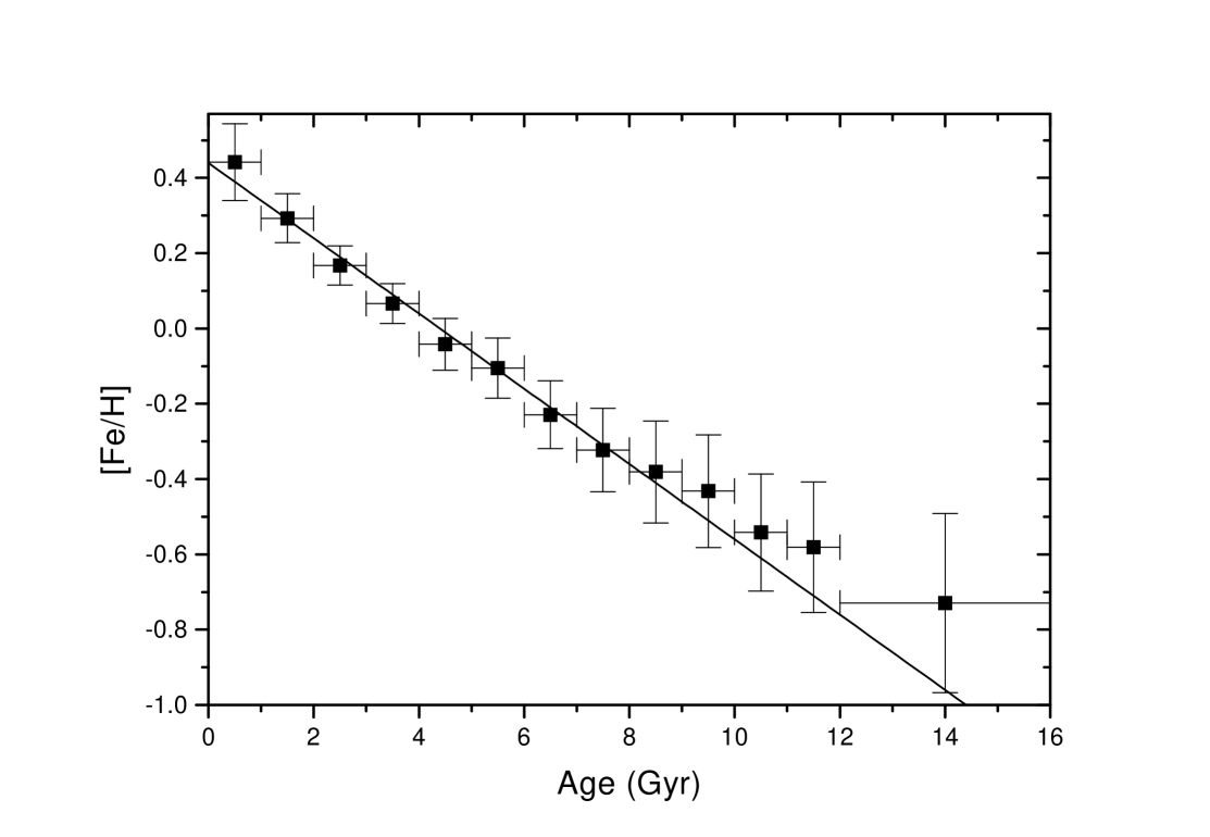
The simulations were repeated 20 times. The results are very similar from one simulation to the other, and one sample simulation is shown in Figure 15. It can be seen that the AMR found with the chromospheric ages follows closely the real AMR of the disk up to 9 Gyr ago, when it begins to deviate. The deviation is always in the sense of an increased dispersion and higher mean AMR. This is exactly the same that is observed in the AMR we have found for the disk. On the other hand, these simulations show that even in face of great age errors, the AMR can be fairly well recovered from a sample with chromospheric ages.

The increase of metallicity dispersion at the older age bins, as well as the greater deviation from the real AMR, are all consequences of the age errors. The older bins tend to be populated by the poorer stars, and the corrections to the chromospheric ages (Rocha-Pinto & Maciel RPM98 (1998)) increase very much for metal-poor stars. A small error in [Fe/H] or $\log R^{\prime}_{\rm HK}$ reflects in a substantial error in age, which most probably will push the star to greater chromospheric ages. Due to this effect, the oldest age bins are more likely to be depopulated by metal-poor stars than the other bins. That is why the recovered AMR fails to match the original AMR as we consider ages progressively older. And the metallicity dispersion increase because the absolute age errors increases as a function of age.

In our simulations we have found that the average metallicity of the oldest bin is invariably around 0.20-0.23 dex higher than the real average metallicity, due to the age errors. If we apply this value to the Milky Way AMR derived previously, we get a disk initial metallicity around $-0.70$ dex, which agrees very well with Edv93’s AMR and with the G dwarf metallicity distribution.

4 Metallicity dispersion

4.1 Some Evidences for a Non-Homogeneous Interstellar Medium

The metallicity dispersion we have found is about 0.13 dex as shown by the error bars of Figure 14 and from Table 3. It is much lower than that found by Edv93. At first sight, this result seems to revitalize old ideas about the chemical evolution of our Galaxy, in which the interstellar medium has been continuously and homogeneously enriched by metals ejected by the stars. Previous works on the AMR (Twarog twar (1980); Meusinger et al. meu (1991)) have consolidated this view by finding $\sigma_{\rm[Fe/H]}$ around 0.12-0.18 dex.

This picture was strongly questioned after Edv93 published their detailed work on the chemical evolution of the disk. They found a larger dispersion in the AMR, varying from 0.18 to 0.26 dex. A number of hypotheses to explain it were considered, and the main conclusion of the authors is that a significant part of this scatter could be physical. Infall is quoted as one of the best mechanisms that could drive such an intrinsically large metallicity dispersion at all epochs, if the time scale for the mixing of the infalling gas is greater than that of star formation. The viability of the infall hypothesis requires star formation to be much more efficient in the material that has just fallen onto the disk than in the already well-mixed gas. This would occur if infall could drive star formation. It is interesting to see that a number of theoretical and observational evidences favour this process (Lépine & Duvert lep94 (1994); Lépine et al. lep99 (1999)), although a detailed study of this star formation mechanism connected with a chemical evolution model has never been made.

Figure 16: Comparison between photometric and spectroscopic metallicities for Edv93’s stars. The photometric metallicity for them was estimated as described in subsection 2.2.

An alternative explanation was proposed by Wielen et al. (WFD (1996)) and Wielen & Wilson (wiewil (1997)) according to which the metallicity dispersion in Edv93’s AMR originated from the diffusion of the stellar orbits (Wielen wielen (1977)). According to this hypothesis, the Sun was born 1.9 kpc closer to the galactic center in comparison with its present position. This could solve a long-lasting puzzle about the fact that the Sun is richer than some younger neighbour objects (Cunha & Lambert cunha (1992); de Freitas Pacheco camisa12 (1993)). Clayton (clayton (1997)) also used this scenario to explain the meteoritic abundance ratios of the isotopes ²⁹Si and ³⁰Si, related to ²⁸Si.

Recently, Binney & Sellwood (binney (2000)) reconsidered the diffusion of stellar orbits and found that, a typical star is unlikely to migrate from the galactocentric radius of its birthplace by more than 5% over its lifetime. These authors say that Wielen et al. (WFD (1996)) calculated the diffusion of stellar orbits in velocity space, adopting isotropic and constant diffusion coefficients. When the diffusion is calculated in integral space, it becomes very anisotropic. As a result, the star does not change significantly the guiding-center radius of its orbit, which should be similar to $R_{m}$, as in Edv93. This recent work concludes that the metallicity scatter in Edv93 is probably real.

The existence of some scatter in the interstellar medium is not questioned. The Sun-Orion abundance discrepancy and the existence of young stars with subsolar abundance (Grigsby, Mulliss & Baer grigsby (1996)) are classical puzzles that point to the existence of an intrinsic metallicity dispersion in the galactic gas. The real problem is its quantification, since these anomalies can be outliers.

For instance, Binney & Sellwood (binney (2000)) show data measured by other authors, which indicate that the intrinsic scatter in [O/H] should be around 0.10 dex. Garnett & Kobulnicky (garnett (2000)) also conclude that, from measurements in nearby galaxies and the local ISM (Kennicutt & Garnett KG96 (1996); Kobulnicky & Skillman KS96 (1996); Meyer, Jura & Cardelli meyer (1998)), the metallicity scatter is lower than 0.15 dex.

4.2 Isochrone-spectroscopic data vs. chromospheric-photometric data

The average metallicity dispersion we have found is very close to that found by Twarog (twar (1980); $\sim 0.12$ dex). Twarog’s sample is greater than Edv93’s and has a good statistical significance, but his metallicities are less accurate. Moreover, his ages were found by old, now outdated, isochrones. The problem can be summarized as follows: photometric AMRs show a small, well-behaved metallicity scatter (however, see Marsakov et al. marsakov (1990)), while the only one based on a spectroscopic sample indicate the opposite. Note that Ng & Bertelli (ng (1998)) only revisit Edv93’s ages, so that their AMR cannot be taken as an independent evidence for a real greater scatter.

It is important to show that there is no significant difference in the quality of our data compared to those of Edv93, even taking into account that our metallicities are photometric and our ages are chromospheric. In Figure 17, we show the comparison between the 16 stars in common between ours and Edv93’s sample, before and after the application of the metallicity corrections to the chromospheric ages (Rocha-Pinto & Maciel RPM98 (1998)). Note that these corrections improve substantially the matching between both methods to measure the stellar ages. The exceptions are few, and will be discussed separately.

Figure 17: Comparison between isochrone and chromospheric ages for 16 stars in common between this work and Edv93. a) before the application of the metallicity corrections to the chromospheric ages (Rocha-Pinto & Maciel RPM98 (1998)); b) after the application of the metallicity corrections. The few deviating stars are discussed in section 4.3.

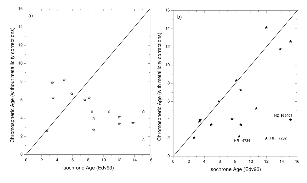
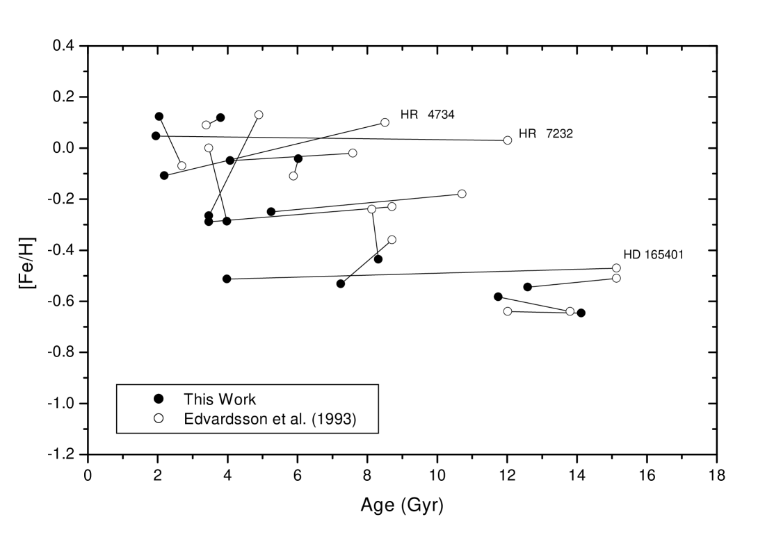
The agreement is also good for metallicities. In Figure 18, the position of our stars in the age–metallicity diagram is shown. Lines connect these stars with their position in the same diagram using Edv93’s data. With only one exception, all stars present differences in metallicities that are within the expected error in the photometric calibration of [Fe/H].

Sixteen stars is a small number to test if our method to estimate ages and [Fe/H] is good. We have chosen to compare directly these methods to estimate stellar ages and metallicities, using the stars in Edv93’s sample.

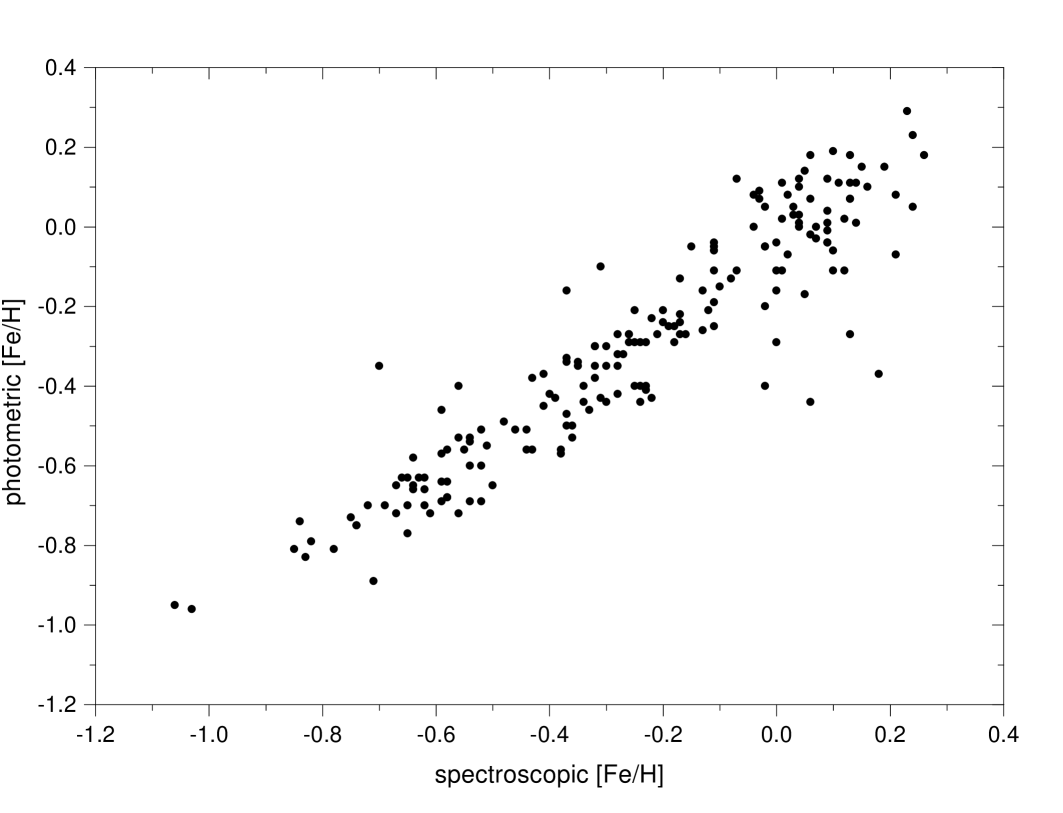
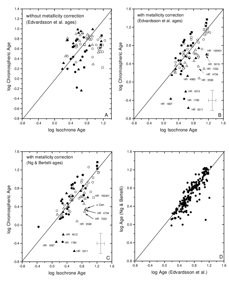
The first of these comparisons is shown in Figure 16, where we show the correlation of photometric and spectroscopic metallicities for the 189 stars in Edv93 sample. The photometric metallicity was estimated as described in the subsection 2.2. The agreement is typical of that expected from a photometric calibration. The standard deviation of the data is 0.10 dex.

Figure 18: Age–metallicity diagram showing the position of the 16 stars in common between this work and Edv93. The lines connect the same stars as they appear using photometric plus chromospheric data and isochrone plus spectroscopic data. With only one exception, all stars present differences in metallicities that are within the expected error in the photometric calibration of [Fe/H].

Chromospheric indices were published only for 81 stars from those of Evd93 sample, and 40 of them were used in the determination of the metallicity correction to the chromospheric age (Rocha-Pinto & Maciel RPM98 (1998)). We present, in Figure 19, a comparison between the isochrone and the chromospheric ages, before and after the application of the metallicity corrections. The stars are distinguished by symbol (according to their spectroscopic metallicity) and style (if it was already used by Rocha-Pinto & Maciel RPM98 (1998) or not). The Figure shows clearly that the metallicity corrections improve substantially the chromospheric ages. The scatter is comparable to the expected error in both methods (we use here a formal average error of 0.1 dex for Edv93 ages, although Lachaume et al. lach (1999) have shown that this error can be easily underestimated). Panel c of Figure 19 shows the same comparison, now using Ng & Bertelli (ng (1998)) ages. The agreement is somewhat better, although a greater isochrone age is still found for some stars. Panel d shows a comparison, in the same scale, between the isochrone age determinations by Edv93 and Ng & Bertelli (ng (1998)).

Isochrone ages are better compared to chromospheric ages, at least for early G dwarfs (Lachaume et al. lach (1999) showed that this is not true for intermediate and late G darfs). The difference can be large, but in general, it is of the same order as the difference between two isochrone age determination made using different isochrones (see panel d of Figure 19). This Figure shows that the error estimate in Fig. 5 is fairly reasonable. They are considerably large, but they are not expected to destroy the AMR, as shown by our simulation in Figure 15.

There are only three stars that were classified as subgiants in Figure 1, that have both a chromospheric and isochrone age. For two of them (HD 9562 and HD 131117), the ages agree remarkably to within 0.15 dex. The third star (HR 4734 = HD 108309) is investigated in more detail in what follows. On the other hand, Edv93’s sample has some slighlty evolved subgiants, which are represented by the oldest stars in Figure 19. The good agreement between their chromospheric and isochrone ages shows that the chromospheric activity–age relation can be extrapolated to slightly evolved subgiants.

4.3 Anomalies to the chromospheric activity–age relation

Few stars deviated significantly from the expected relation in panels b and c of Figure 19. With two exceptions (HR 1780 and HD 165401), all of them have metallicities greater than $-0.05$ dex. The deviation is in the same direction: stars that appear to be very young, according to their chromospheres, are found to be much older from their position in the HR diagram. Three of these stars (HR 4734, HR 7232 and HD 165401) were measured only once by the Mount Wilson group, according to Duncan et al. (duncan (1991)). While their high chomospheric activity could be caused by a periodic active phase in their magnetic cycles, all of the other stars were observed more than a hundred times, over a time span of 12 years or more, and errors in the chromospheric indices cannot be invoked to explain their different ages.

Figure 19: Comparison between chromospheric and isocrone ages for 81 Edv93’s stars. The different symbols stand for: stars with [Fe/H] $\leq-0.50$ (squares), stars with $-0.50<{\rm[Fe/H]}\leq-0.10$ (circles), and stars with [Fe/H] $>-0.10$ dex. The styles indicate whether the star was already used to correct the chromospheric age scale (open symbols) or not (solid symbols). The upper panels show a comparison between the isochrone and the chromospheric ages, before and after the application of the metallicity corrections. Clearly it can be seen that the metallicity corrections improve substantially the chromospheric ages. The scatter is comparable to the expected error in both methods. Panel c shows the same comparison, now using Ng & Bertelli (ng (1998)) ages. Panel d shows a comparison, in the same scale, between the isochrone age determinations by Edv93 and Ng & Bertelli (ng (1998)).

Some of the deviating stars in panel b are chromospherically young, kinematically old stars (hereafter referred as CYKOS), that have been recently investigated by some of us (Rocha-Pinto, Castilho & Maciel RPCM (2000)). Their origin is presently unknown. Poveda et al. (allen (1996)) have also found objects like these amongst UV Ceti stars, and they proposed they could be low-mass blue stragglers, formed by the coalescence of close binaries. Other explanation could be that these stars are themselves close, unresolved binaries. The high rotation rates of these systems tend to keep the chromospheric activity well beyond the normal age where we would expect it to have been diminished. Moreover, systematic chemical variations between them and the other normal stars could be a cause for some deviations from the relation. However, we have found no such difference, using the abundance ratios provided by Edv93. We can but conclude that these stars do not follow the chromospheric activity–age relation. A possibility to be explored by future investigations is whether the metallicity correction to the chromospheric ages of the metal-rich stars have been overestimated. It is apparent from Figure 1 of Rocha-Pinto & Maciel (RPM98 (1998)) that some metal-rich stars present great difference between their chromospheric and isochrone ages.

The existence of anomalies to the chromospheric activity–age calibration does not throw doubt about the use of chromospheric indices to measure stellar ages. The exceptions are few. There are also exceptions to the use of photometric indices to measure stellar parameters, for instance in peculiar stars, but these do not rule out the validity and quality of photometrically calculated parameters. The difference is that there are ways to photometrically distinguish between a normal from a peculiar star. But this is not possible for CYKOS from chromospheric indices alone. We are not sure whether it could be done by photometry. The only way to discover a CYKOS presently is by comparing their activity levels with their isochrone ages and their kinematical characteristics.

4.4 The problem of the metallicity scatter

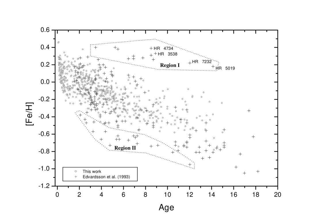
A more instructive way to compare the metallicity scatter of the two AMR is presented in Figure 20, where we superpose both AMR’s. The differences occur mainly in two regions, which we have marked by dotted lines, and named as Region I and II. Region I has also other interesting characteristic: it is well detached from the bulk of stars in both samples. Note that four stars amongst those that have deviated from the mean relation in Figure 19 are also present in Region I. It suggests that the other stars in this location do not follow the chromospheric activity–age relation. We have chromospheric indices for five other stars in this region (HR 3176, HR 3951, HR 5423, HR 8041 and HR 8729). All of them also present chromospheric ages lower than their isochrone ages, although the age excess is smaller than that found for the stars in Figure 19. Table 4 presents the logarithmic isochrone age of these stars ($\log I_{\rm age}$), in Gyr, taken from Edv93, and the age excess ($\Delta$), which we define as the logarithmic difference between the isochrone and the chromospheric age of a star (see Rocha-Pinto & Maciel RPM98 (1998)). For other star, HR 2354, chromospheric indices were not found in the literature, but emission in the Ca II K line was observed by Hagen & Stencel (hagen (1985)). Significant X-ray emission was also observed by the ROSAT observatory (Hünsch, Schmitt & Voges hunsch (1998)), confirming that it is chromospherically active. Its spectral type is G3 III-IV. Although Micela, Maggio & Vaiana (micela (1992)) showed that the X-ray activity can be used as an age indicator in giants, no study has ever aimed to calibrate an age relation for them. We have used the relation proposed by Kunte, Rao & Vahia (kunte (1988)) to estimate an X-ray age for it. We alert that this relation was calibrated only for main-sequence stars, and its use here is merely illustrative. Using the value for the X-ray luminosity over bolometric luminosity given by (Hünsch, Schmitt & Voges hunsch (1998)), we have an X-ray age of 2.5 Gyr to HR 2354, which is lower than the isochrone age found by Edv93, just like for the other stars with chromospheric ages.

Table 4: Age excesses for stars in Region I and II of Edv93’s AMR.

Name	$\log I_{\rm age}$	$\Delta$
Region I
HR 2354a	$0.84$	$0.44$
HR 3176	$0.94$	$0.31$
HR 3538	$0.95$	$0.87$
HR 3951	$0.81$	$0.48$
HR 4734	$0.93$	$0.59$
HR 5019	$1.15$	$0.55$
HR 5423b	$0.84$	$0.53$
HR 7232	$1.08$	$0.79$
HR 8041b	$0.89$	$0.48$
HR 8729	$0.93$	$0.53$
Region II
HR 4657	$0.73$	$0.32$
HR 5447	$0.32$	$-0.17$
HR 8354	$0.75$	$-0.32$
a Age estimated by X-ray luminosity (Hünsch et al. hunsch (1998))
b Chromospheric indices given by Young et al. (young (1989))

The presence of CYKOS in this region also points to a wrong age determination (both isochrone and chromospheric), since as a coalesced star, as an unresolved close binary would have both chromospheric activity and position in the HR diagram uncorrelated with its real age. This can explain why there is a gap between Region I and the other stars. Chromospheric indices for other stars in this region could test more properly this hypothesis.

The other region marked in Figure 20 corresponds to the metal-poor stars with young to intermediate ages. None of such stars are present in our AMR. This could be explained if there were some systematic error in the metallicity corrections to the chromospheric ages that would avoid locating stars in this region. Unfortunately, there are chromospheric measurements for only three stars in Region II. Their age excesses do not follow a systematic trend, as for the stars in Region I, as can be verified in Table 4.

We have checked if the scatter in our AMR could have been partially destroyed due to the use of the metallicity corrections. Rocha-Pinto & Maciel (RPM98 (1998)) have proposed such a correction from their finding that the difference between chromospheric and isochrone ages were related to the stellar metallicity. The correction itself disregards the scatter in the data. If this scatter is real, probably reflecting different chemical compositions, the use of a calibrated metallicity correction could remove partially the dispersion in the chromospheric AMR. We have used a simulation analogous to that used in the previous section. This time, we have used a ‘AMR’ composed only by scatter, that is, 730 stars were randomly distributed in age (from 0 to 16 Gyr) and metallicity (from $-1.2$ to 0.4 dex). We have taken explicitly into account the dispersion in the metallicity correction, taken from Figure 1 of Rocha-Pinto & Maciel (RPM98 (1998)), as well as the errors in $\log R^{\prime}_{\rm HK}$ and [Fe/H]. We have found that the chromospheric AMR preserves closely the real metallicity dispersion of the data, even with the greatest possible scatter for the disk AMR.

Figure 20: AMRs from Edv93 (crosses) and from this work (open circles). The major differences correspond to two areas in this diagram where we have found no stars, while Edv93 found some. These regions were named I and II, and are marked by dotted lines. The stars labelled have also shown peculiar behaviour in Figure 19.

We have found no indication that the differences in the AMR are due to difference in the methods used to estimate age and metallicity. We are left with the hypothesis that one of the samples (Edv93’s or ours) is not suitable to investigate this constraint.

There are arguments to suspect that Edv93’s sample selection has biased their results. Their sample was selected very carefully to allow the study of the abundance ratios evolution. It is not suitable to other studies such as, for instance, the metallicity distribution. Part of the scatter in Edv93’s AMR comes from their selection procedure to have nearly equal number of stars in predetermined $\delta m_{1}$ intervals, to assure a good coverage of [Fe/H] values in their sample. The authors themselves make a correction for this, using a metallicity distribution of 446 dwarfs, after which the metallicity dispersion diminishes to around 0.21 dex. While this value is closer to previous estimates of the metallicity dispersion in the solar vicinity, it is still greater than ours. What is generally not recognized is that the same kind of problem can occur in the investigation of the metallicity dispersion inside each age bin.

We have tested this with a number of artificial samples. We have deliberately selected randomly nearly 25 stars in each of the metallicity bins that Edv93 used, amounting 189 stars just like their sample, from a set of 2000 artificial stars. These pre-selected AMRs were compared with other AMRs composed by 189 stars randomly selected from the same parent population. We have verified that contrary to the expectation, this kind of selection procedure does not necessarily imply a metallicity scatter greater than what would be found with a more unbiased selection procedure. However, there is a significant difference between these simulations and the procedure made by Edv93. According to them, they had observed the 25 brightest stars in each metallicity box, after disregarding binaries and stars rotating faster than 25 km/s. This probably causes a bias that was not taken into account by the authors. If there was a one-to-one relation between metallicity and age, the age of the 25 brightest stars would be the same as that of the 25 faintest stars. On the other hand, if there is a real metallicity scatter in the interstellar medium, at the same metallicity, the brightest stars would not have the same age dispersion as the faintest stars, or the age dispersion of a subsample randomly selected. The brightest stars will be generally the nearer stars and the most evolved, which are higher in the HR-diagram. From stellar evolutionary theory we also know that these are generally the older stars, or the hotter stars. Since Edv93 also avoid faster rotating stars (which corresponds to the hotter stars), the majority of these stars will be old. Therefore, Edv93’s metallicity bins have probably non-representative age distributions, which changes the whole dispersion in the AMR.

This selection effect was introduced by intrinsic observational limitations. Other selection effects are also present in their sample due to this problem. For instance, Garnett & Kobulnicky (garnett (2000)) have shown that there is a distance bias in Edv93’s sample. Stars at distances 30-80 pc from the Sun are systematically metal-poor. The explanation for this trend is provided by Edv93 themselves. To have equal number of stars in each metallicity bin, they observed the metal-poor stars at a large volume. Garnett & Kobulnick conclude that the real scatter in the AMR should be lower than 0.15 dex, which favours our results. Edmunds eddy (1998) favours the same conclusion.

However, the puzzle cannot be considered solved. It is highly necessary to have an independent study of the spectroscopic AMR, preferably using a sample as large as that of Twarog. It is also important to make a more detailed investigation of the link between age and stellar activity, especially for the CYKOS and other deviating stars. Presently, we can conclude that the photometric, chromospheric AMR does not give support to the great scatter in the AMR as found by Edv93. Therefore, the AMR can be still regarded as a strong constraint to chemical evolution models, just like the G dwarf metallicity distribution and the radial abundance gradients (see Chiappini, Matteucci & Gratton chiappini (1997)).

5 Conclusions

We have used an extended sample composed of 552 late-type dwarfs, with chromospheric ages and photometric metallicities, to address the AMR of the solar neighbourhood. Our main conclusions can be summarized as follows:

1. The AMR is found to be a smooth function of time. The average metallicity has increased by at least 0.56 dex in the last 12-15 Gyr. No absence of rich stars ageing 3 to 5 Gyr, as suggested by Carraro et al. (carraro (1998)), was found. The results are in fairly good agreement with the mean points of Edv93’s and Ng & Bertelli (ng (1998))’s AMR.

2. The initial metallicity of the disk was around $-0.70$ dex. This suggests some previous enrichment of the gas which gave rise to the thin disk.

3. A number of very metal rich stars in Edv93 could be composed by chromospherically young, kinematically old stars (CYKOS). These stars could originate from coalesced stars or unresolved close binaries. This may indicate that their isochrone ages, as measured by Edv93, are wrong. This can, at least, explain why Edv93 have found some old stars more metal rich than the Sun.

4. An average intrinsic metallicity dispersion of 0.13 dex was found. Several hypotheses were tested to explain this scatter compared to that found by Edv93. We have found no indication that it could be produced by our method to estimate ages and metallicities. On the other hand, this dispersion agrees closely with the recent conclusions by Garnett & Kobulnicky (garnett (2000)) that the real scatter in the AMR should be lower than 0.15 dex. Nevertheless, additional independent determinations of the AMR are strongly encouraged to confirm this view.

Some important bias in the sample can be investigated with the aid of kinematical data. A third paper on this series addressing this topic is being planned.