Weak Lensing by High-Redshift Clusters of Galaxies - I: Cluster Mass Reconstruction

Abstract

We present the results of a weak lensing survey of six high-redshift ($z>0.5$), X-ray selected clusters of galaxies. We have obtained ultra-deep $R$-band images of each cluster with the Keck Telescope, and have measured a weak lensing signal from each cluster. From the background galaxy ellipticities we create two-dimensional maps of the surface mass density of each cluster. We find that the substructure seen in the mass reconstructions typically agree well with substructure in both the cluster galaxy distributions and X-ray images of the clusters. We also measure the one-dimensional radial profiles of the lensing signals and fit these with both isothermal spheres and “universal” CDM profiles. We find that the more massive clusters are less compact and not as well fit by isothermal spheres as the less massive clusters, possibly indicating that they are still in the process of collapse.

1 Introduction

High-redshift clusters of galaxies are very powerful tools for testing the predictions of cosmological and structure formation models. The mere existence of high-mass, X-ray luminous clusters at $z>0.5$ strongly constrains many models (Eke, Cole, & Frenk 1996) while the presence of a $\sim 10^{15}M_{\odot}$ cluster at $z\sim 0.8$ makes unlikely many $\Omega_{0}=1,\Lambda=0$ cold dark matter models (Luppino & Gioia 1995; Bahcall, Fan, & Cen 1997; Henry 1997). Even stronger constraints can be placed on the model once details of the clusters such as mass surface density, cluster galaxy ages, amounts of sub-clustering, and mass-to-light ratios are known (Crone, Evrard, & Richstone 1996; Trentham & Mobasher 1998).

It has been only recently, however, that these high-redshift, high-mass clusters have been able to be detected. Optical surveys tend to find low-mass clusters and often mistake the superpositioning of unrelated groups of galaxies as clusters (Reblinsky & Bartelmann 1999). Further, until recently, the optical surveys were either too small to reasonably expect to find a high-mass, high-redshift cluster or were not deep enough to detect the high-redshift cluster galaxies.

X-ray observations, however, have proven to be an efficient way to detect these clusters. The Einstein Extended Medium-Sensitivity Survey (EMSS) found five $z>0.5$ high-mass ($>$ few $\times 10^{14}M_{\odot}$) clusters (Gioia & Luppino 1994), and various ROSAT surveys are finding many more (Henry et al.  1997, Gioia et al.  1999, Burke et al. 1998, Vikhlinin et al.  1998, Rosati et al.  1998). The X-ray surveys not only provide clusters which are truly of high-mass, and not a superposition of unrelated groups of galaxies, but also provide a means to measure the masses of the clusters. These masses have been used to apply constraints to cosmological and structure formation models (Henry 1997), but are subject to an uncertainty in that the masses measured from the X-ray emission of the clusters depend on the dynamical state of the cluster (Evrard, Metzler, & Navarro 1996).

We, therefore, have undertaken an optical survey of these X-ray selected, high-redshift clusters to perform weak lensing analysis on the clusters. Our primary goals in doing this survey are threefold: First, we wish to measure the masses of the clusters using weak lensing, which does not have a dependence on the dynamical state of the cluster. Second, we wish to determine the dynamical state of the clusters and detect any substructure in the clusters. Finally, we wish to determine the redshifts of the faint blue galaxy (FBG) population which is used in the weak lensing analysis.

We selected as our sample of clusters the five EMSS high-redshift clusters (MS $0015.9+1609$ at $z=0.546$, MS $0451.6-0305$ at $z=0.550$, MS $1054.4-0321$ at $z=0.826$, MS $1137.5+6625$ at $z=0.782$, and MS $2053.7-0449$ at $z=0.583$), which were the only $z>0.5$ clusters published from a serendipitous X-ray survey at the time, and one from the ROSAT North Ecliptic Pole survey (RXJ $1716.6+6708$ at $z=0.809$) which was discovered shortly after we began our survey (Henry et al.  1997, Gioia et al.  1999). We have already published early results on the clusters MS $1137.5+6625$ and RXJ $1716.6+6708$ (Clowe et al.  1998). In this paper we will present the weak lensing data of the other four clusters as well as a correction to the mass profiles published in Clowe et al.  (1998). We will discuss how the redshift distribution of the FBG population can be constrained with the weak lensing observations in a future paper (Paper II).

In §2 we present the weak lensing theory used in our analysis. Our observations and details of the data reduction processes are given in §3. In §4 we discuss the properties of the clusters and the weak lensing results. Section 5 contains our conclusions. Throughout this paper, unless otherwise stated, we assume an $\Omega_{0}=1,\Lambda=0$ cosmology, assume $H_{0}=100h$ km/s/Mpc, and give all errors as 1 $\sigma$.

2 Weak Lensing Theory

It is well known that massive objects, such as clusters of galaxies, will bend light-rays passing by them with their gravitational pull. If there is a good alignment between the positions of the background galaxy and the center of mass of the cluster of galaxies then the background galaxy can be strongly lensed. In strong lensing, the galaxy is imaged into an arc, or a series of arcs, along critical curves by magnifying the galaxy’s size tangentially to the cluster center of mass. By measuring the redshifts of the cluster and the arc, one can determine the mass of the cluster interior to the arc, and also characteristics of the lensing such as time delays between various images (Schneider, Ehlers, and Falco 1992).

If the background galaxy is not well aligned with the cluster center of mass lensing will still occur. This lensing, however, will only slightly distort the shape of the background galaxy, increasing the galaxy’s size tangential to the cluster center of mass. If the background galaxies were all circular in shape then this weak distortion would be easily detected. Because the background galaxy population has an intrinsic ellipticity distribution (the dispersion of which is much higher than the change introduced by the gravitational distortion), however, this weak lensing distortion can only be detected by looking for a statistical deviation from a zero average ellipticity tangential to a center of mass from a large number of background galaxies. Because of the intrinsic ellipticity distribution of the background galaxies and that each image has a finite number density of background galaxies, weak lensing reconstruction is an inherently noisy process as the sample of background galaxies will not have an average intrinsic ellipticity that is precisely zero.

Weak lensing, however, has two distinct advantages over other methods traditionally used to measure cluster masses. The first advantage is that weak lensing provides a direct measure of the surface density independent of the dynamical state of the cluster. The other advantage is that the strength of the weak lensing signal is directly proportional to the surface density and thus can, in theory, be used to measure the surface density of structures much smaller than, for instance, X-ray imaging whose emissivity scales as the square of the density.

2.1 Basic Equations

The goal of weak lensing observations is to measure the dimensionless surface density of the clusters, $\kappa$, where

$$\kappa={\Sigma\over\Sigma_{crit}}.$$ (1)

$\Sigma$ is the two-dimensional surface density of the cluster, and $\Sigma_{crit}$ is a scaling factor:

$$\Sigma_{crit}={c^{2}\over 4\pi G}{D_{s}\over D_{l}D_{ls}}$$ (2)

where $D_{s}$ is the angular distance to the source (background) galaxy, $D_{l}$ is the angular distance to the lens (cluster), and $D_{ls}$ is the angular distance from the lens to the source galaxy. The surface density is related to the gravitational surface potential $\phi$:

$$\kappa={1\over 2}\nabla^{2}\phi={1\over 2}(\phi_{,11}+\phi_{,22}).$$ (3)

The surface density $\kappa$ cannot, however, be measured directly from the shapes of the background galaxies. Instead, one can measure the mean distortion in the galaxies by looking for a systematic deviation from a zero average ellipticity. From the distortion one can measure the reduced shear $g$ (details given in the next section), which is related to the shear $\gamma$ by

$$g={\gamma\over 1-\kappa}$$ (4)

(Miralde-Escude 1991). In the weak lensing approximation, it is assumed that $\kappa<<1$. Under that assumption and that the background galaxies have an isotropic intrinsic ellipticity distribution the distortion measured in the galaxies can be translated to a shear by a direct scaling. The shear $\gamma$ is related to the surface potential $\phi$ by:

$$\gamma_{1}={1\over 2}(\phi_{,11}-\phi_{,22})$$

$$\gamma_{2}=\phi_{,12}.$$ (5)

While the lensing distorts, and enlarges, the background galaxy, it preserves the surface brightness of the background galaxy. As a result, the total luminosity of the background galaxy is increased proportional to the increase in its surface area. The increase of the size of each axis of the galaxy is simply $(1-\Lambda_{i})^{-1}$ where $\Lambda_{i}$ are the eigenvalues of $\phi_{,ij}$, which is equivalent to $[(1-\kappa)-\gamma]^{-1}$ for the axis tangential to the cluster center of mass, and $[(1-\kappa)+\gamma]^{-1}$ for the axis radial to the cluster center of mass for the weak lensing regime. Thus, the overall increase in area, and the amplification of the background galaxy luminosity, is:

$$A=|(1-\kappa)^{2}-(\gamma^{2}_{1}+\gamma^{2}_{2})|^{-1}.$$ (6)

One method to convert the measured shear field to a surface density is to Fourier transform the data and convert the Fourier transform of the shear, $\tilde{\gamma}$, to that of the convergence, $\tilde{\kappa}$. There are a variety of ways to do this, but the most useful form is

$$\tilde{\kappa}={(\hat{k}_{1}^{2}-\hat{k}_{2}^{2})\tilde{\gamma}_{1}+2\hat{k}_{1}\hat{k}_{2}\tilde{\gamma}_{2}\over\hat{k}_{1}^{2}+\hat{k}_{2}^{2}}$$ (7)

which has a flat noise power spectrum (Kaiser 1996). One can then inverse Fourier transform to get an estimate of the surface density. This method, originally in Kaiser & Squires (1993, hereafter KS) and hereafter called the KS93 algorithm, has a biasing at the edges of the frame, particularly in the corners, as it assumes an infinite spatial extent of the finite data field (Schneider 1995). Given that the images in our sample are centered on the clusters and that structures of interest are typically restricted to the central half of the images, this will not have a large effect on our results. The KS93 algorithm, however, is only able to measure the convergence to within an additive constant, the mean surface density of the field (normally called the mass sheet degeneracy). As the biasing at the edges would interfere with attempting to fit the observed surface density with a chosen model to determine the mean surface density of the field, we will use this method only to look for substructure and not attempt to measure a mass.

One can also measure the surface density using aperture mass densitometry, which measures the one dimensional radial mass profile from an arbitrarily chosen center, (Fahlman et al.  1994). The traditional statistic used is

$$\zeta(r_{1},r_{m})=\bar{\kappa}(<r_{1})-\bar{\kappa}(r_{1}<r<r_{m})={2\over(1-r_{1}^{2}/r_{m}^{2})}\int_{r_{1}}^{r_{m}}d\ln r\langle\gamma_{T}(r)\rangle$$ (8)

where $\langle\gamma_{T}(r)\rangle$ is the azimuthal average of the galaxy ellipticity component measured with axes tangential and radial to the center of mass at radius $r$ from the center of mass, and provides a lower bound on the surface density interior to radius $r_{1}$. However, because this statistic subtracts $\bar{\kappa}$ of the annulus outside $r_{1}$, the final measured mass $M(<r_{1})=\pi r_{1}^{2}\zeta(r_{1})\Sigma_{crit}$ depends not only on the strength of the detected lensing signal but also on the mass profile of the cluster. In particular, any substantial substructure or secondary core in the cluster would change from being included in the mass estimate to being subtracted, at a reduced level, as $r_{1}$ moves inward across the structure. This would cause the measured slope of the mass profile at this point to be shallower than what is actually present. One can easily modify the statistic to

$$\zeta_{c}(r_{1},r_{2},r_{m})=\bar{\kappa}(<r_{1})-\bar{\kappa}(r_{2}<r<r_{m})=2\int_{r_{1}}^{r_{2}}d\ln r\langle\gamma_{T}\rangle+{2\over(1-r_{2}^{2}/r_{m}^{2})}\int_{r_{2}}^{r_{m}}d\ln r\langle\gamma_{T}\rangle$$ (9)

which subtracts a constant $\bar{\kappa}(r_{2}<r<r_{m})$ for a fixed inner annular radius $r_{2}$ for all apertures in the measurement, thereby removing any potential error from extended structures as mentioned above. The measured mass profile $M(r_{1})=\pi r_{1}^{2}\zeta_{c}(r_{1})\Sigma_{crit}$ is now the mass of the cluster minus an unknown, but presumably small, constant times $r_{1}^{2}$. While the value of the additive constant for aperture densitometry is not known, one knows what the constant physically is, namely the average surface density of an annular region at some radius around the center of the cluster. By modeling the mass distribution of the cluster, one can hopefully get a good estimate of the value of this constant.

All of the above equations assume that one can provide a direct measure of the shear. As one can only measure the reduced shear $g$ (eqn 4), all of these methods will measure a value for the convergence which is too large. Further, the ratio of the measured value to the true value of the convergence increases with increasing convergence, and thus a profile of the convergence would be measured to be much steeper than it actually is. The KS93 algorithm can be corrected for this effect by first estimating the convergence field by assuming the measured reduced shear is the true shear, and then iteratively approximating the shear as $g(\vec{r})(1-\kappa(\vec{r}))$ where $\kappa(\vec{r})$ is taken from the latest iteration (Seitz & Schneider 1995). While the aperture densitometry profiles can also be corrected using an iterative technique, as one uses a model to calculate the value of $\bar{\kappa}$ in the annular region it is easier to simply calculate the $\zeta$ and $\zeta_{c}$ for the models using the reduced shear for comparison to the profile.

Even though $\zeta_{c}$ has a single constant subtracted from all the bins, it is not necessarily always better to use than $\zeta$. A simple calculation of the signal to noise ratios of the two statistics, assuming a constant background galaxy density, only one source of lensing in or near the field, and a surface density with a power law fall-off ($\kappa\propto r^{-n}$) gives

$${\zeta_{c}/\sigma_{\zeta_{c}}\over\zeta/\sigma_{\zeta}}={(r_{2}^{n}-r_{1}^{n})(r_{m}^{2}-r_{1}^{2})\over r_{2}^{n}r_{m}^{2-n}(r_{m}^{n}-r_{1}^{n})}+{r_{1}^{n}(r_{m}^{2}-r_{1}^{2})(r_{m}^{n}-r_{2}^{n})\over r_{2}^{n}(r_{m}^{n}-r_{1}^{n})(r_{m}^{2}-r_{2}^{2})}$$ (10)

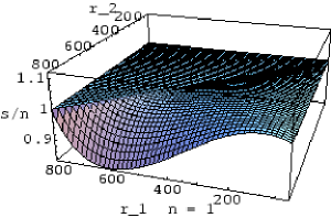
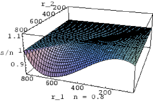
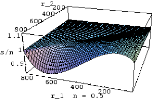
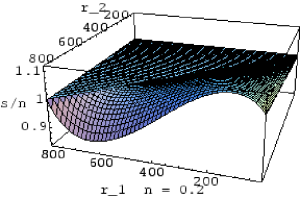
Figure 1: Signal-to-noise ratio of the aperture densitometry statistics. This plot shows the ratio of ${\zeta_{c}/\sigma_{\zeta_{c}}\over\zeta/\sigma{\zeta}}$ as a function of $r_{1}$ and $r_{2}$ for four different signals with power-law surface densities $\kappa\propto r^{-n}$. $r_{1}$ and $r_{2}$ are given as pixels, and $r_{m}$ is assumed to be at 1000 pixels. As can be seen, the $\zeta_{c}$ statistic tends to have a higher signal-to-noise than the $\zeta$ statistic at the inner radii but is worse at larger radii. $\zeta_{c}$ is also better for mass profiles which are not as concentrated (low $n$).

where $r_{m}$, $r_{2}$, and $r_{1}$ are defined as in eqn 9. As can be seen in Figure 1, at large values of $r_{1}$, the signal-to-noise ratio for $\zeta_{c}$ is worse than that of $\zeta$, but as $r_{1}$ decreases it eventually becomes better than that of $\zeta$. The radius at which $\zeta_{c}$ has a better signal-to-noise ratio depends on both the inner radius of the annulus, $r_{2}$, and $n$, the power law fall-off of the surface density. For an isothermal sphere, $n=1$, $\zeta_{c}$ is generally worse in s/n ratio than $\zeta$ for all but the innermost radii, but tends to do better for smaller values of $n$.

2.2 $\kappa$ Reconstruction From Images

The previous section deals mainly with how one can transform the gravitational shear to a surface density. For real data, however, one also needs a mechanism to convert the background galaxies’ ellipticities, which can be measured directly from the images, to a gravitational shear value. To measure the ellipticities of the galaxies we used a weighted second moment of inertia such that

$$e=\left[\begin{array}[]{c}{Q_{11}-Q_{22}\over Q_{11}+Q_{22}}\\ {2Q_{12}\over Q_{11}+Q_{22}}\end{array}\right]$$ (11)

where

$$Q_{ij}=\int d^{2}\theta W(\theta)\theta_{i}\theta_{j}f(\theta)$$ (12)

where $\theta$ is measured relative to the center of the object (defined by the centroid of the surface brightness), $f(\theta)$ is the surface brightness of the object, and $W(\theta)$ is a weighting function (in this case a Gaussian)(KS). One of the nice aspects of this method of defining the ellipticity is that, in the weak lensing regime, at every point there will be some set of axes for which $e_{1}$ will be changed by the gravitational shear while $e_{2}$ will remain the same as the pre-shear value (or vice versa). If one can determine the orientation of these axes, such as the radial and tangential directions around a circularly symmetric lens, then by averaging over many galaxies, one of the ellipticity components can be used to measure the shear while the other would provide a measure of the intrinsic ellipticity distribution of the galaxies.

It is, in theory, quite easy to convert the measured ellipticities into a shear field. Kaiser, Squires, & Broadhurst (1995) (hereafter KSB) have shown that the shear field will change the ellipticity of an object by

$$\delta e_{\alpha}=P_{\alpha\beta}^{\gamma}\gamma_{\beta}.$$ (13)

The quasi-tensor $P_{\alpha\beta}^{\gamma}$ is an observable quantity which can be calculated from the object image (KSB, corrections in Hoekstra et al.  1998). This calculation was made in the weak lensing approximation ($\kappa<<1$); to use this in the inner regions of massive clusters where the weak lensing approximation does not hold, one needs to replace the shear $\gamma$ with the distortion $g$. Given that the mean ellipticity of the background galaxies should be 0, one has

$$g_{\beta}=\left<{(P_{\alpha\beta}^{\gamma})^{-1}e_{\alpha}}\right>$$ (14)

where the brackets indicate averaging in a chosen manner over the area of interest.

2.3 High Redshift Lenses

Because $\Sigma_{crit}$ depends on $D_{s}/D_{ls}$, high redshift cluster lenses have an additional complication over lower redshift lenses. For low redshift ($z_{l}<0.3$) cluster lenses, $\Sigma_{crit}$ is effectively the same for all background galaxies with redshifts several times higher than the lens. Thus, by taking an image deep enough to have most of the background galaxies in the sample at $z\gtrsim 0.7$, all of the galaxies can be treated as being at the same redshift, and all will be magnified and distorted by the same amount. For higher redshift clusters, $z>0.5$ in particular, this is not the case, and $\Sigma_{crit}$ continues to decrease fairly rapidly across the redshift range in which most faint galaxies are thought to reside ($1<z<4$). This variation in the lensing strength as a function of background galaxy redshift provides not only some complications in the analysis, but also a potentially useful tool to determine the redshift distribution of the background galaxies, which will be discussed in paper II.

The first complication is that because $\Sigma_{crit}$ is no longer constant for all the background galaxies one must compute a mean value to convert the measured $\kappa$ to a surface density. From eqn 1, one has

$$\left<\kappa\right>=\Sigma\left<{1\over\Sigma{crit}}\right>=\Sigma{{\int_{z_{1}}^{z_{2}}n(z)dz\over\int_{z_{1}}^{z_{2}}{n(z)\over\Sigma_{crit}(z)}dz}}$$ (15)

where $n(z)$ is the number of galaxies in the sample at redshift $z$. Of course, eqn 15 assumes a knowledge of the redshift distribution of the background galaxies, which is currently known spectroscopically to only $z\approx 1$ (eg: Songaila et al.  1994, Koo et al.  1996, Cohen et al.  2000). Thus, for clusters with $z>0.5$, for which background galaxies with $z>1$ must be used to measure a weak lensing signal, one can only measure a mass for the cluster by guessing at the redshift distribution of the background galaxies or, if one has enough passbands, estimating the redshift of each object using photometric redshifts (eg: Hogg et al.  1998).

The other complications created by the dependence of the strength of the lensing on the redshifts of the background galaxies are all due to the fact that, in addition to having the shapes of the galaxies distorted, the sizes of the galaxies are enlarged while the surface brightness remains constant, thereby magnifying the total luminosity of the galaxies. Because the greater the lensing strength the greater the magnification of the background galaxy aperture luminosity, any constant magnitude selection of background galaxy population will have the redshift distribution slightly altered from that of the unlensed background galaxy population (Broadhurst, Taylor, & Peacock 1995). This results in the lensed population having a larger fraction of higher redshift galaxies, and thus the mean redshift of the background galaxy population will have increased. Because the strength of the lensing signal depends on both the mass and the redshift of the cluster, both of these will affect the $n(z)$ for the background galaxy population. If no correction is made for this effect, then the more massive clusters will be measured to be even more massive than they truly are, and higher redshift clusters will be measured to be more massive than the lower redshift clusters of the same mass.

Another consequence of the magnification is that, because the strength of the lensing signal increases as the distance from the center of the cluster decreases, $\bar{\Sigma}_{crit}$ is not constant over the full extent of a cluster (Fischer & Tyson 1997). Without knowing the redshift distribution of the background galaxies as a function of magnitude, one cannot even predict whether $\bar{\Sigma}_{crit}$ will become larger or smaller as a function of radius (Broadhurst, Taylor, & Peacock 1995). This effect, however, should only be important near the cluster core (i.e. at large $\kappa$).

All of these effects can be corrected for if the redshift distribution of the background galaxies is known. Currently, however, the redshift distribution for field galaxies is known only to $z\approx 1$, which is much smaller than the expected redshifts of the background galaxies in the images of this sample. Unlike Fischer & Tyson (1997), we will not adopt a theoretical model to predict the redshift distribution of the background galaxy population. Instead, we simply provide our results with the caveats that the higher redshift clusters will have a higher measured surface density than lower redshift clusters of the same mass and that there might be a correction needed to the surface densities of the cluster cores. In both cases, however, we expect that the corrections for galaxy magnification will result in a change of less than $20\%$ of our measured surface densities.

3 Observations

Luppino and Kaiser (1997) (hereafter LK) show that for high-redshift clusters, most of the weak lensing signal comes from the faint blue background galaxies. The cluster galaxies, however, are quite red in color over the optical wavelengths. Thus, in order to maximize the ability to distinguish cluster galaxies from the background galaxies used in the weak lensing analysis, the observations need to be taken in as red a band as possible, and in at least two different bands to allow rejection of cluster and foreground galaxies based on color. Further, because LK did not see any significant lensing until background galaxy magnitudes $I\geq 23.5$, the observations need at least one color as deep as possible to get a signal-to-noise on the background galaxies large enough to accurately measure the ellipticities of the galaxies.

The Low Resolution Imaging Spectrograph (LRIS, Oke et al.  1995) at the Keck Observatory was judged to be ideal for this task. It has a large enough field of view ($6\arcmin\times 8\arcmin$) to allow imaging outside the core of high-redshift clusters without having to mosaic large offsets together, and has enough light gathering power (with the 10 meter primary mirrors of the Keck telescopes) to image the faint background galaxies in only a few hours of integration per field. However, because the $I$-band filter on LRIS was designed to not have a long wavelength cutoff, the $I$-band images taken with LRIS tend to exhibit large fringing effects. As we were not sure this fringing was stable and could be easily removed without affecting the quality of the images, we choose to use the $R$-band as our primary observation band. $I$-band and $B$-band images were obtained from the UH88^′′ telescope using the Tek2048² CCD, which has a field of view and pixel size similar to that of LRIS.

A list of the nights observed and data taken is given in Table 1. All the data were taken using a “shift-and-stare” technique in which short exposures (300s on Keck, 600s in $I$ and 900s in $B$ on the UH88^′′) were obtained with small dithers ($\sim 15\arcsec$) between each exposure. Standard star observations and calibration frames were also obtained for each night of observation. The data were obtained during nights which were mostly photometric. The magnitudes of bright but unsaturated stars were used to determine which images were non-photometric. Those images which had stars significantly fainter ($>0.1$ magnitudes) than average were rejected from the following analysis. Typical seeing was $0\farcs 6$ to $0\farcs 8$.

3.1 Image Reduction

The following image reduction routine was performed on all the data taken after each observing run. If all the nights had the same characteristics (seeing, sky brightness, cloudiness, etc) then the entire run was processed at the same time, otherwise each night was processed separately.

The first step was the creation of a master bias frame from the bias frames taken at the beginning and ending of each night. The pixel values of the master bias frame were the median of the pixels in each bias frame after rejecting those pixels which were more than three $\sigma$ from the median. This rejection removed any cosmic rays present in the bias frames before the median was computed. The master bias frame was subtracted from each data and standard star frame.

The over-scan region for each frame was averaged to a single column and a linear least squares fit was performed on the column. A three $\sigma$ rejection routine was then performed on the over-scan column to remove any values increased by a star on the edge of the CCD, and the linear least squares fit for the column was recomputed. The fit was subtracted from each column of the CCD data to remove any dark current and fluctuation in the bias value over the course of the night. In every case, the amount subtracted using the over-scan regions after the master bias subtraction was less than 15 ADU, or about 1$\%$ of the value of the bias.

The images were trimmed to the 2048$\times$2048 pixel physical CCD area, and rotated, if necessary, so that north was increasing row numbers and east was decreasing column numbers. For the Keck images, which have the right and left hand sides of the chip vignetted (at 0^o rotation angle), a clipping of the first 215 and last 233 columns was performed, with all the pixels in those columns being set to a value which indicated that they should be ignored for all future operations on the images. The clipped region was slightly larger than that physically vignetted to remove any fringing on the edges of the fields.

A flat field image was created for each band from the median of the data images with sky level greater than one hundred times that of the read noise of the CCD. As with the creation of the master bias, while medianing the data images, the pixels with values more then three times the standard deviation of the median were rejected and the remaining pixel values were re-medianed. The flat field image was then divided by the mean value of the image so that the average pixel value in the flat field image was unity. Each data and standard star image was divided by the normalized flat field for the band. This removed quantum efficiency and through-put variations across the image.

A bad pixel mask was created by combining the pixels which had a bias value of greater than one third the full well capacity of the CCD with the pixels which had a value in the flat field which was less than one fourth the average value (or, in other words, masking out those pixels which would give a signal-to-noise less than one half that of the average pixel on the CCD). The bad pixel mask was then used to mask all of the data and standard star images. This masking set all of the “bad” pixels on the CCD to a value which indicated to the averaging and analysis routines that the pixel should be automatically excluded from any measurements.

The sky was then fitted and subtracted from all of the data and standard star images. This was accomplished by finding all the local minima across the CCD and placing these in a smaller image, so that each pixel value in the new image was the sum of the minima in the pixel range which was binned to make the sky pixel. A second image was also made which was the number of minima used to create each sky pixel. The two images were then convolved with a Gaussian to remove high frequency noise and gaps in the sky coverage. The summed sky value image was then divided by the number of minima image to obtain a final value for each pixel, which was then subtracted from the original image. In addition to removing any low frequency sky variations, this routine typically removed large wings of very bright, saturated stars in the images as well as any large, low surface brightness objects which might have been present. It also would have removed any cD halos around the brightest cluster galaxy of the clusters, but those regions were edited so that the sky around the BCG was an extrapolation of the region outside that being edited (typically $\sim$20 pixel radius.)

A less robust version of the object finding routines described in §3.3 was used to measure the centroid positions, fluxes, and half-light radii for all the stars in the frames. Data frames which showed a larger half-light radius than the average (bad seeing) were excluded from the sample. The stellar centroid positions were used to calculate the offsets and any distortion corrections. For the UH88″ $I$- and $B$-band frames, there was no significant distortion detected, and so the offsets were a simple linear shift, with possibly a small rotation angle for data sets taken on two different runs. For the Keck $R$-band frames, however, a very large distortion correction was needed to remove the effects of the curved focal plane and the distortions introduced by the LRIS reimaging optics. These distortion corrections were calculated by mapping the stellar centroids onto those for the summed $I$-band image, and fitting a bi-cubic polynomial to minimize the differences in the two positions. The stars selected for the registration had $20<R<23$, which were bright enough to have rms errors in the centroid less than 0.05 pixels ($\sim 0\farcs 01$), determined from simulations of placing the stars on a Guassian random noise background with the same rms as the observed sky noise and calculating the centroid. The internal rms error on the corrected positions was typically $\sim 0.08$ pixels (compared to the positions of the same stars in the other frames), and agreed with the positions in the $I$-band image at $\sim 0.1$ pixels (which is the error in the centroids in the $I$-band image due to higher sky noise).

The images were undistorted and shifted into the common registration frame as defined by the offsets calculated above. Whenever a fractional pixel shift was needed, a linear interpolation over the pixel and the neighboring pixels was performed. The amount added to each post-shift pixel was calculated by integrating the interpolation over the region of the pre-shift pixel overlapping each post-shift pixel. The post-shift pixels were then divided by the fractional area of the pre-shift pixels contained within them in order to preserve surface brightness. This technique was tested to ensure that the second moments of the objects were not changed by the fractional pixel shifts, except of course in the case of the distortion correction.

The now registered images were then averaged after a 4$\sigma$ rejection routine was performed on all the stacked pixels to remove cosmic rays and moving objects. It is interesting to note that because the Keck telescopes have an alt-az mounting system, the diffraction spikes seen coming from bright stars because of deflection of the stellar light off of the secondary mirror spider supports rotate as the field moves across the sky. As a result, the rejection routine removed the stellar spikes from the $R$-band images, thus removing the chance that these might be detected as objects by the detection routines described in §3.3.

The last step in the image reduction is to compare the fluxes in the standard stars, all of which are taken from Landolt (1992). The exposure times for the standard stars were calculated so that the charge in the central pixel would be large, but still within the linear e^-/ADU regime on the CCD. The stellar flux was measured using an aperture large enough to include the radius at which the flux becomes smaller than the sky noise, but small enough to not include any nearby objects. The sky level was calculated for each star by creating a histogram of the pixel values in an annular region around the star and fitting a Gaussian using a low weight for the pixel values greater than the point at which the histogram drops below $\text@frac{3}{4}$ the peak value on the high side of the median. Any bad pixels within the half-light radius of the standard star invalidated the star’s use, while any bad pixels outside the half-light radius but within the aperture radius for the star were replaced with a linear interpolation from the surrounding pixels. Finally, for the Keck images, only those standards within the central 1024 pixels were used to prevent a possible systematic error based on an incorrect distortion correction.

3.2 Object Detection and Analysis

After creating an added image, the next step in the weak lensing analysis is measuring the parameters of all the objects in the image. We used the IMCAT object detection and analysis package (available at http://www.ifa.hawaii.edu/$\sim$kaiser/imcat) to perform most of the steps described below.

The first step was to detect all the various galaxies and stars in the image. This was done using a hierarchical peak-finding algorithm, which smoothes the image using progressively larger mexican-hat filters. By comparing the peak positions of the increasingly smoothed images, not only can the positions of the objects be detected, but also a rough estimate of their size based on the smoothing radius at which the peak is lost to the noise or combined with another nearby peak (KSB). The technique is much better at finding small, faint objects and large, low surface brightness objects than the single aperture size scanning method of FOCAS (Jarvis and Tyson 1981) and other similar programs, but tends to produce a large number of detected noise spikes and often has problems with both grouping together galaxies which are projected near each other and breaking large spiral galaxies into smaller pieces. The noise spikes, however, are easily removed from the catalogs by size and signal-to-noise cuts, and for purposes of this paper the large foreground spirals were excluded from the analysis of background objects, so it does not matter in how many pieces such galaxies are detected. Further, because the detections of a pair (or more) of nearby galaxies as a single object only occurs a small fraction ($\approx 1\%$) of the time, these objects can also be excluded from the catalogs without any biasing of the results or significant reduction in the signal-to-noise of the weak lensing signal.

The next step was to determine the sky level around each object which was determined from an annulus around the object with an inner radius of $16\times r_{g}$, where $r_{g}$ is the smoothing radius at which the object achieved maximum significance, and an outer radius of $32\times r_{g}$. This annulus was broken into four equal size regions by radial divisions, and the mode pixel value for each quadrant was determined. From these mode values the average sky level was determined, along with a two-dimensional linear slope for the sky level. A very large object, such as a bright star or a foreground galaxy, could of course increase the mode of the pixels in a quadrant, so usually all pixels within $3\times r_{g}$ of another object were excluded from the mode calculation.

Once the sky value was known, an aperture flux and magnitude was calculated. The flux was determined by summing all the pixels inside an aperture of $3\times r_{g}$ after subtracting the sky level as determined above. This choice of aperture radius is large enough to count almost all of the light from the object, but small enough to (usually) avoid including any light from nearby objects. Any pixels within $2.5\times r_{g}$ of another object were excluded from the aperture. Bad pixels were not corrected for but were noted in the catalog of objects, and thus any objects with bad pixels in them could easily be excluded (although this happened only for saturated stars, objects overlapping a saturation spike of a very bright star, and objects on the very edges of the summed image). The aperture magnitude was then calculated from the flux and a zero-point magnitude determined from the standard stars. A half-light radius, the radius at which the integrated flux is $\text@frac{1}{2}$ the aperture flux, was also calculated.

The object shapes were determined by calculating the second moments of the light distribution as given by eqn 12, using a circular Gaussian with a standard deviation equal to $r_{g}$. The centroid of the object was calculated by minimizing the first moments of the weighted surface brightness, using the same Gaussian weighting function as above. The second moment is then used to calculate the ellipticity of the object as given in §2. The centroid position was then used as the position of the objects, instead of that found in step 1. This made little difference in the weak lensing analysis as the two positions were different on average by only 0.1 pixels. Any objects with positional differences larger than 0.4 pixels ($\approx$ 4 times the error in the centroiding algorithm) were excluded from the catalog as probably being either a multiple object detection or an object having an unusual morphology which would not have a normal ellipticity. This rejection tended to remove about $2\%$ of the objects in the catalog.

The next step in the analysis was to remove from the catalog of objects noise spikes, saturated stars, and groups of objects detected as a single object. This was done by rejecting objects which had bad pixels inside their aperture, objects which were extremely small (typically $r_{g}<1.6$ pixels for 0$\farcs$7 seeing and 0$\farcs$22 pixels), objects which were overly large ($r_{g}>10$ pixels), objects which were very faint ($R$-band magnitudes $>28$), and objects which had large ellipticities ($e>0.5$). The remaining objects in the catalog were then checked manually against the summed image to remove any object groups which managed to pass all of the above tests.

The final step in the object analysis was to obtain the sky level and aperture photometry on the objects detected in the Keck $R$-band images for the $B$- and $I$-band images.

3.3 Background Galaxy Selection

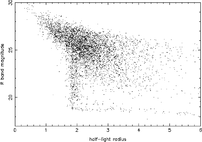
Figure 3: A plot of $r_{h}$, the radius which encloses half of the detected light from a object, versus the total magnitude of the objects detected in the MS $2053.7-0449$ field is shown above. Galaxies (foreground, background, and cluster) form a broad swath across the plot while stars, all having roughly the same measured half-light radius, lie in a tight finger in plot. By using this plot, moderately bright stars can easily be separated from galaxies, although faint galaxies and stars blend together.

Once a catalog of all the objects (stars, foreground, cluster, and background galaxies) was generated, the next step was to isolate the background galaxies and to correct for seeing and anisotropies in the point spread function. The stars are very easy to separate from the galaxies by using a half-light radius vs. magnitude plot. As can be seen in Figure 3, the galaxies form a broad diagonal swath in the plot while the stars are concentrated around a single half-light radius value, and are clearly separated from the galaxies for the brighter stars. Thus by separating the objects in this “finger” on the plot, the brighter stars can be isolated from the rest of the catalog. Further, because any saturation of the star or the core of the star falling into the non-linear response area of the CCD will increase the half-light radius, it is easy to remove saturated stars from the star catalog.

The next step was to separate the background galaxies from the cluster and foreground galaxies. Because the redshifts of the galaxies in these images are only sparsely sampled, it is impossible to fully distinguish between the three groups of galaxies. Figure 4 shows a color vs. magnitude plot for all the detected objects in one of the fields, MS $1054.4-0321$. At bright magnitudes, almost all of the detected galaxies (almost certainly foreground galaxies) lie in a narrow color band of $.6<R-I<1.1$. Around $R=22$ a second narrow color band appears with $1.3<R-I<2.0$, which are the cluster galaxies (the brightest cluster galaxy in this field has a color of $R-I=1.6$). The $z\sim 0.55$ cluster galaxies are not quite as red as the $z\sim 0.8$ cluster galaxies shown, with typical colors of $0.9<R-I<1.5$. At fainter magnitudes, starting around $R=24$, the non-cluster galaxies begin to break into two groups. One of the groups stays in a narrow color range, but the color as a whole gets redder, eventually merging with and then surpassing the $R-I$ colors of the cluster galaxies. The other group forms a broad swath of galaxies bluer than the foreground galaxies. While it appears from Figure 4 that the faint red galaxies outnumber the faint blue galaxies, the opposite is in fact true. Because the $I$-band images are not as deep as the $R$-band images, most of the faint galaxies are not detected in the $I$-band images but are assumed to be bluer than those which are detected.

In order to have the background galaxies in each cluster analysis drawn from the same redshift distribution, we applied the same selection criteria for all of the fields. In order to remove the $z\sim 0.5$ cluster galaxies and have the background galaxy population have most of its population at $z>0.8$, we used those galaxies with $23<R<26.3$ and $R-I<0.8$. This resulted in a number density in the background galaxy catalog between 33 and 42 galaxies/sq. arcminute. The spread in background number density is larger than the expected variation due to Poissonian noise, and is due to incompleteness at the faint end for the images with smaller exposure times and possibly to the presence of faint blue cluster galaxies, particularly for the $z\sim 0.8$ clusters, in the final selection. All further attempts at refining the selection using additional colors resulted in a lowering of the signal-to-noise of the lensing signal.

3.4 Correction for Seeing and Distortion

Once the background galaxy sample has been selected, the last step before the weak lensing analysis programs could be applied was to correct the ellipticities of the galaxies for atmospheric seeing and telescope distortion. The primary effect of the seeing is that the ellipticities of the galaxies have been reduced because the original shape of the galaxy has been smeared by the nearly-circular point spread function. Small anisotropies in the seeing along with aberrations (such as coma and wind shake) in the telescope focal plane can cause an apparent shear which must be removed from the data, otherwise a false mass signal will be generated during the weak lensing analysis.

Because the stars are near point-sources before the light enters the atmosphere and they are not being lensed by the cluster in the image, the shapes of the stellar profiles in the image are caused by the effects that need to be removed from the galaxy profiles. Thus, one can measure the ellipticities and sizes of the stellar profiles and can use these to correct the galaxy profiles. This can be done in a manner very similar to that used to describe how galaxies would respond to an applied shear given in §2.2. One can calculate from each object a quasi-tensor $P_{\alpha\beta}^{s}$ such that

$$\delta e_{\alpha}=P_{\alpha\beta}^{s}p_{\beta}$$ (16)

(KSB, corrections in Hoekstra et al.  1998). Thus, $p_{\beta}$, which is an analog of the shear field $\gamma$ for the anisotropic smearing, can, in theory, be derived from the ellipticities of the stars in the image. The ellipticities of the galaxies near those stars could be corrected to what they would be for a circular psf. In practice, the shot noise of the stars creates some noise in the second moments used to calculate the ellipticities. Thus instead of using each star to correct the galaxies around it, we fit the ellipticities of the stars as a two-dimensional polynomial as a function of position. Each galaxy’s position can then be used to calculate the ellipticity of the stellar field at that spot, and thus the correction to the galaxy’s ellipticity could be calculated. Shown in Figure 5 are the ellipticities of the stars in the MS $2053.7-0449$ field both before and after the fitted ellipticity correction. The faint galaxies also have a large error in $P_{\alpha\beta}^{s}$ caused by sky and shot noise on the galaxies, but simulations have shown that a better recovery of the circularized psf ellipticity is obtained using each galaxy’s $P_{\alpha\beta}^{s}$ than by trying to calculate an ensemble average for galaxies with a similar size, ellipticity, and orientation. This is due mainly to the fact that one can construct two objects to have the same size, ellipticity (as measured by second moments), orientation, and total luminosity, but have radically different morphology, and thus they would deform differently under an applied smearing kernel.

Once the object shapes have been corrected to a circular psf, the next step is to remove the dilution of the ellipticity caused by the smearing of the object by the psf. Because the $P_{\alpha\beta}^{\gamma}$ is measured for the objects after the seeing has been applied, one cannot use the method of §2.2 to obtain the shear. LK have shown, however, that effects of seeing can be removed using

$$g_{\beta}=\left<e_{\alpha}(P^{\gamma}_{\alpha\beta}-P^{s}_{\alpha\delta}P^{\gamma\ast}_{\delta\epsilon}{P^{s\ast}_{\epsilon\beta}}^{-1})^{-1}\right>$$ (17)

where an asterisk denotes the value for the stars in the frame.

Because the object ellipticities have been altered since the $P$ values were calculated, the measured $P$ values are no longer valid. Calculating the correct $P$ values for the ellipticity corrected objects is non-trivial (and near impossible for faint objects because of the sky noise), so instead we use ${P^{\gamma}_{\alpha\beta}}^{\prime}={1\over 2}(P_{11}^{\gamma}+P_{22}^{\gamma})\delta_{\alpha\beta}$ and ${P^{s}_{\alpha\beta}}^{\prime}={1\over 2}(P_{11}^{s}+P_{22}^{s})\delta_{\alpha\beta}$. In doing this conversion, we are making two assumptions about how the P values change. The first is that the off-diagonal terms are small compared to the on-diagonal terms, and thus can be ignored. The second assumption is that the size of the objects does not change when doing the ellipticity corrections, so the trace of the $P$ values remains the same after the corrections.

This technique was tested on simulated data which was first sheared, then convolved with a Gaussian psf. The standard data analysis package was used on both the sheared, pre-seeing image and the post-seeing image. As can be seen in Figure 6, the recovered shear from both images is nearly identical.

3.5 Simulations

One of the goals of the study was to determine the dynamical state and detect any substructure in the clusters. The aperture densitometry profiles will be somewhat useful in this regard as they can determine if the radial profiles of the clusters are similar to those expected from collapsed objects. Of more use, however, would be to detect and measure the mass of any structures not part of the cluster cores. To do this, however, the noise levels in the mass reconstructions must be calculated.

The largest non-systematic noise source in weak lensing analysis is the intrinsic ellipticity distribution of the background galaxy population. Thus, the level of noise in the mass reconstructions depends primarily on the background galaxy density. It does, however, also have a significant dependence on the image quality (how sharp the psf is). Because of the inherent shot noise in the flux detected from the galaxies and the brightness of the night sky, there is an unavoidable error in measuring the second moments of the background galaxies, and thus their ellipticities. Further, due to the fact that worse “seeing” (a larger psf) results in a larger correction factor as described in §3.4, the error in corrected ellipticities is greater for poorer quality images. This increased error not only reduces the measured signal, but also can create large noise spikes from only a handful of galaxies in which the noise has tangentially aligned their ellipticities about some point. The shapes of these noise spikes are usually small and round, although extended structures have been seen in some simulations. They are most easily detected using aperture densitometry, in which they show a signal only over a limited range of radii. By using simulations, however, we can compare the size and strength of features seen in the cluster mass reconstructions to those in simulations and get an estimate for the significance of the features.

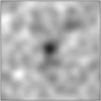
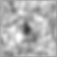
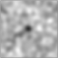
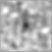
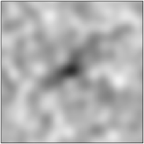
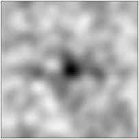
Figure 7: Shown above are nine mass reconstructions generated with the KS 93 algorithm for a simulated isothermal lens ($\sigma=1000$ km/s, $z_{lens}=0.8,z_{bg}=1.5$). As can be seen, the central peak is always distinguishable above the level of the noise, but is usually somewhat elliptical in shape, and often displaced by a small amount from the center of the field. All of the above images are of the same model lens, the differences in the images are a result of the random ellipticities of the background galaxies.

An example of these simulations is shown in Figure 7. These simulations were created using 1960 galaxies (40 galaxies per sq. arcminute) randomly placed on a 7′$\times$7′ field. Each galaxy was given an ellipticity drawn randomly from the pool of all of the background galaxies in the six fields in the survey. The position and ellipticity of each galaxy were then altered to simulate being lensed by a 1000 km/s singular isothermal sphere located in the center of the field assuming $z_{lens}=0.8$ and $z_{bg}=1.5$. Thus, all structures in these simulations which are not part of the singular isothermal sphere lens are a result of noise. The sizes of these structures can then be compared with those in the cluster mass reconstructions to get a measure of the significance of the structures.

4 Cluster Properties

In Table 2 we list the redshifts, X-ray luminosities (converted to a rest frame 0.3 - 3.5 keV band) and temperatures, and the velocity dispersion of galaxies for the clusters in the sample, all of which are taken from the literature. We also give the $R$ magnitude of the brightest cluster galaxy (BCG) within a 10$h^{-1}$ kpc radius circular aperture and cluster galaxy number counts and Abell richness class. All of the galaxies we chose as BCGs have been spectroscopically identified as being a member of the cluster (Carlberg et al. 1996; Donahue et al.  1998, 1999; Gioia & Luppino 1994). The cluster galaxy number counts and corresponding Abell richness class were measured following the prescription of Bahcall (1981) in which all galaxies within two magnitudes fainter than the third brightest cluster member and less than 250$h^{-1}$ kpc from the BCG were counted. The number of background galaxies was estimated using the same magnitude selection of galaxies at the edges of each image and scaled by the ratio of areas between the two samples. This estimate was subtracted from the observed number counts around the BCG. The errors for the number counts in Table 2 are based on Poissonian noise for the background galaxy counts and errors in the photometry of the third brightest cluster galaxy and the fainter galaxies which could cause galaxies to move into or out of the magnitude limits. The third brightest cluster galaxy was chosen by finding the third brightest object within 250$h^{-1}$ kpc of the BCG which was extended compared to the psf and had a $R-I$ color within .3 magnitudes of the BCG ($\sim 1.3$ for the $z\sim 0.55$ clusters and $\sim 1.6$ for the $z\sim 0.8$ clusters).

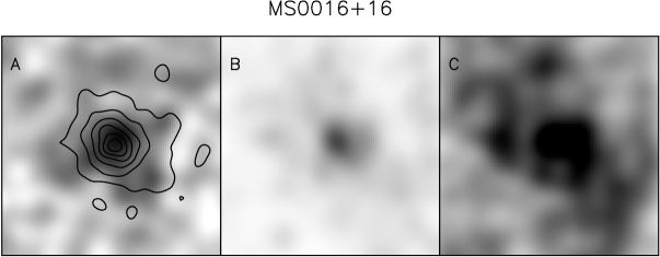
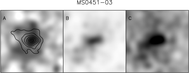
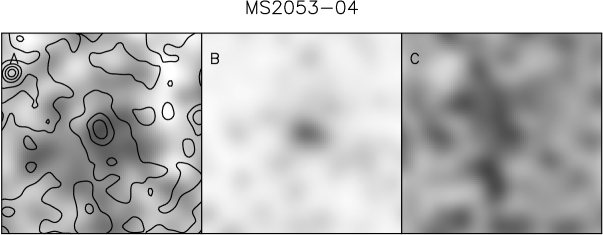
Figure 8: Mass surface density, color-selected galaxy luminosity and number count map of the $z\sim 0.55$ clusters are shown above. The mass reconstructions from the KS93 algorithm are labeled A, and the galaxy luminosity and number count maps are labeled B and C respectively. The maps are all $5\farcm 9$ on a side (same as the color images in Figures 12-15) and have all been smoothed by a 17″Gaussian. The grey-scale of the maps is the same in all maps displaying the same quantity (all mass reconstructions, etc.).

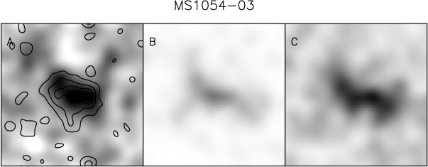
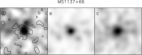
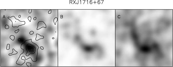
Figure 9: Mass surface density, color-selected galaxy luminosity and number count map of the $z\sim 0.8$ clusters are shown above. The mass reconstructions from the KS93 algorithm are labeled A, and the galaxy luminosity and number count maps are labeled B and C respectively. The maps are all $5\farcm 9$ on a side (same as the color images in Figures 12-15) and have all been smoothed by a 17″Gaussian. The grey-scale of the maps is the same in all maps displaying the same quantity (all mass reconstructions, etc.) and are the same as in Figure 8.

The KS93 mass reconstructions for the clusters are shown in Figures 8 ($z\sim 0.55$ clusters) and 9 ($z\sim 0.8$ clusters). The reconstructions are 352″ in width (1300$h^{-1}$ kpc at $z=0.55$ and 1450$h^{-1}$ kpc at $z=0.8$) and have been smoothed by a Gaussian filter with a $17\farcs 6$ standard deviation. The number density of background galaxies used to make these mass maps for each cluster are given in Table 2. Overlayed in contour on the mass maps are X-ray images of the fields from ROSAT HRI observations, smoothed by the same Gaussian filter as the mass map (Neumann & Böhringer 1997; Donahue 1996; Donahue et al.  1998, 1999; Gioia et al.  1999). Also shown in Figures 8 and 9 are the distribution of galaxies with R-I colors within .3 magnitudes of the BCG weighted by $R$-band luminosity and by number. Both images are smoothed by the same Gaussian filter as the massmap.

A profile, centered on the BCG, of the reduced shear and aperture densitometry for each cluster is shown in Figure 10. The outer radius of the profiles is the distance from the BCG to the nearest edge of the R-band image. The minimum radius from the BCG was chosen to be 100$h^{-1}$ kpc, which is large enough to still have a usable number of background galaxies for shear estimation but is sufficiently far from the Einstein radius (the radius at which $\bar{\kappa}=1$ and strong lensing occurs) that the approximation for the reduced shear used in §$2.2$ is still valid. The reduced shear profiles were fit with both “universal” CDM profiles (Navarro, Frenk, and White 1996, hereafter NFW), integrated to a surface density (Bartelmann 1996) and isothermal sphere profiles using a $\chi^{2}$ determination for quality of fit and assuming that the background galaxies lie in a sheet at $z_{bg}=1.5$. The parameters of the best fit for each model as well as the $\chi^{2}$ and significance from a zero mass model for each cluster are given in Table 2. It should be noted that the NFW models are not robust fits, as the two parameters can be adjusted against each other to some extent and not severely decrease the quality of the fit, as can be seen in Figure 11. While the parameters describing the best fit depend on the assumed redshift of the background galaxies, changing this assumed redshift will not alter the quality of the fit of the profiles or the significance from a zero mass model. Changing the assumed redshift of the background galaxies will also change the mass computed from the measured $\bar{\kappa}$ in the aperture densitometry profiles.

4.1 MS $0015.9+1609$

MS $0015.9+1609$ is the most well-known of the clusters in our sample. It was originally discovered by R. Kron in 1975 (Koo 1981) and has served as a high-redshift cluster in most every survey since (eg: Dressler et al.  1997, Smail et al.  1997, Yee et al.  1996). It was included in the EMSS, which was a serendipitous and not targeted survey, because it was in the field of another targeted cluster (Gioia and Luppino 1994, hereafter GL). A composite three-color image of the cluster is given in Figure 12.

Optically, the cluster is very easy to recognize with three bright galaxies in a line running north-east to south-west, the BCG being the central galaxy of the three, surrounded by a large number of fainter galaxies. MS$0015.9+1609$ has the highest number of color selected cluster galaxies in the sample, but these counts may be enriched by a foreground structure at $z\sim 0.3$ (Ellis et al.  1985). As can be seen in Figure 8, while the three large galaxies cause the smoothed central light peak to be elliptical with the major axis running north-east south-west, the fainter galaxies in the core are distributed circularly about the BCG, with a slight over-density to the west of the BCG. The centroids of both the galaxy counts and galaxy luminosities are slightly south-west of the location of the BCG.

The mass distribution created with the KS93 algorithm is shown in Figure 8. The central peak of the mass distribution is roughly the same size and is in the same location as both the galaxy count and luminosity peaks. There are four “arms” of matter extending radially from the central peak, and three of the arms have analogs in the galaxy count and luminosity maps. The strength of the signal in these arms, however, is barely above the level of the noise objects generated in the simulated fields shown in Figure 7, and thus it is unclear how well they might indicate cluster substructure. The shape of the central peak, however, is very similar to that of the ROSAT HRI observations (Neumann & Böhringer 1997), which is overlayed in contours on the mass reconstruction in Figure 8. The offset between the peaks in the X-ray luminosity and the weak lensing massmap is not significant and is presumably caused by the intrinsic ellipticity distribution of the background galaxies. Similar sized offsets have been seen in the simulations between the reconstructed mass peak and the true mass peak.

Smail et al.  (1995) also performed a weak lensing analysis on this cluster. Their aperture densitometry profile and mass at 300 $h^{-1}$ kpc agree within errors with ours. There is a difference in the shape of the central peak in the mass-maps, but that can be attributed to the difference in the background galaxy populations used to perform the lensing analysis. The difference between the two mass-maps is similar to what is seen in weak lensing reconstruction simulations of the same lensing potential using two different background galaxy populations.

4.2 MS $0451.6-0305$

MS $0451.6-0305$ is the most X-ray luminous cluster in the EMSS (GL). A composite three-color image of the cluster is given in Figure 13.

The core of the cluster is easy to recognize as a large bar of galaxies with a north-west south-east orientation. The brightest cluster galaxy (BCG) is in the middle of the bar, but is the second brightest galaxy in that area due to a foreground galaxy lying just south of it. In both the galaxy count and luminosity maps (Figure 8) the bar-like structure of the core is clearly visible. The centroid of this bar in the galaxy count map is consistent with the location of the BCG, while the centroid of the luminosity map is slightly to the south-east of the BCG due to the galaxies on that side generally being somewhat more luminous than those to the north-west of the BCG. Both maps show that outside the core, the majority of the cluster galaxies are also located either to the south-east or the north-west of the BCG.

The peak of the mass is centered on the BCG, but the broad bar-like structure evident in the galaxy distribution has a much smaller spatial extent in the mass reconstruction. A ROSAT HRI X-ray image of the cluster (Donahue 1996) is overlayed in contours on the mass reconstruction. It also shows the bar-like structure of the core but with a much smaller extent than that of the galaxy distribution. A moderately large northern extension from the central peak present in the mass reconstruction is consistent with a (much weaker) structure seen in the cluster galaxy distribution. Further, most everywhere one can find a maxima in the galaxy distribution, a corresponding mass signal can be found, although most of these are just barely above the level of the noise seen in the simulations.

4.3 MS $2053.7-0449$

MS $2053.7-0449$ has the lowest X-ray luminosity of the $z>0.5$ clusters detected in the EMSS. A composite three-color image of the cluster is given in Figure 14. MS $2053.7-0449$ is much harder to find optically than the rest of the clusters in the catalog given that it is at a lower galactic latitude. A group of moderately bright stars ($15\lesssim R\lesssim 17$) is projected on, and partly obscures, the southern part of the cluster. The brightest cluster galaxy (BCG) is located just above a triangle formed by pairs of stars. The cluster core is plainly evident in the smoothed luminosity image and the centroid of this core is located about 6$\arcsec$ west of the location of the BCG. In the galaxy count image, however, the core is extended in a bar running roughly north-south, and there is a second bar of similar size and density located to the south of the core of the cluster. As a complete redshift catalog has not been compiled for this cluster, it is uncertain as to whether the southern bar structure and a second over-density of galaxies located north-east of the core are associated with the cluster.

The centroid of the central peak is consistent with the location of the BCG. Unlike the other $z\sim 0.55$ clusters, the central peak is not a simple elliptical, but is shaped similar to the letter “c”. While the simulations shown earlier nearly always resulted in the detection of a compact core, they were done with a lensing mass a factor of 3-4 higher than the apparent mass of MS $2053.7-0449$ based on the X-ray luminosity. The smaller central potential results in a greater distortion to the central peak, and in roughly $15\%$ of the simulations with a mass similar to MS $2053.7-0449$’s the central peak was distorted enough that it could no longer be considered to have an elliptical shape. There is a mass detection in the region where the southern bar of galaxies is seen in the galaxy counts.

4.4 MS $1054.4-0321$

MS $1054.4-0321$ is the highest redshift cluster in the EMSS sample, and until recently it was the highest redshift cluster with a detected X-ray flux (Luppino and Gioia 1995). This cluster was previously analyzed in LK using many of the same techniques as here, although the data used were not as deep. Thus we should have the same results as those in LK with allowance for errors caused by a different selection of background galaxies used in the analysis. This provides a good check on the removal of the distortions introduced by the Keck focal plane.

The three color image of the cluster is given in Figure 14. The cluster is very easy to recognize in the image as a broad swath of galaxies running mostly east-west. The brightest cluster galaxy (BCG) is in the middle of the swath. Both the color selected galaxy luminosity and number distribution show the cluster to be long and extended, looking similar to a short filament. As one would expect, the luminosity map is more sharply peaked in the core than the galaxy distribution map, indicating that the galaxies near the core are brighter, and therefore bigger, than the galaxies further from the center of mass for the cluster. The centroids of both the galaxy counts and luminosities are consistent with the position of the BCG. When one uses a smaller smoothing scale than that in Figure 9, the filamentary structure of the core can be broken into three separate peaks. One of these peaks, the largest in both galaxy number counts and luminosity, is centered on the BCG, and the other two are located to the west and north-east of the BCG.

The shape of the central mass peak is extremely similar to the shapes seen in the galaxy count and luminosity maps. As with the cluster galaxy number count and luminosity images, if the mass reconstruction is smoothed on a smaller scale than that shown in Figure 9, the mass peak becomes three different peaks with the central peak being the largest (most massive). No other structures in the mass reconstruction are above the level of the noise seen in the simulations.

The ROSAT HRI image (Donahue et al.  1998) of the cluster also agrees in both position and angle with the galaxy count, luminosity, and weak lensing mass maps for the cluster with the exception that it does not have the small peak north-east of the cluster core and has a maximum in the western, instead of the central, peak. A second ROSAT image (Neumann et al.  2000) has the western peak much smaller which suggests that this might be a variable source or noise. The small southern extension from the cluster core in the X-ray map is not seen in either the weak lensing or color-selected galaxy maps, but could be caused by a foreground source, possibly the star located south-west of the cluster core (Neumann private communication). The fact that three different techniques of tracing mass all show the same non-circular distribution simply provides more compelling evidence that MS $1054.4-0321$ does not have a spherical mass distribution, and may indicate that it is not yet virialized and is just in process of forming.

The weak lensing data presented here agrees very well with that of LK. The shape of the central mass peak in LK is similar to that seen above, although with more noise due to the decreased number of background galaxies available for the analysis. The radial profile also has good agreement, within the errorbars, although, as expected, the Keck data shows a slightly higher $\bar{\kappa}$, which is indicative of the median redshift for the background galaxies being somewhat higher than the background galaxies used in LK.

This cluster has also been recently studied using an HST mosaic image by Hoekstra et al.  (2000). The smaller PSF in the HST images resulted in their being able to obtain a number density of faint galaxies roughly twice what was detected in the Keck image. This allowed them to detect the three components of the cluster core at a higher significance. The weak lensing shear and aperture densitometry profile from the HST data agree within errors with that presented here.

4.5 MS $1137.5+6625$ and RXJ $1716.6+6708$

Our data on MS $1137.5+6625$ and RXJ $1716.6+6708$ were presented in an earlier paper (Clowe et al.  1998). In the aperture densitometry profiles published in that paper, however, we had not accounted for the breakdown of the weak lensing approximation, and thus the given profiles are too compact. After applying the breakdown of the weak lensing approximation to the best fit models for MS $1137.5+6625$, we find that it can be fit well with an isothermal sphere, and thus we withdraw our assertion that the weak lensing results suggest that the cluster is a filamentary structure extending along the line of sight.

5 Discussion

In the previous section we have shown that we were able to measure a weak lensing signal from all six of the clusters in our sample. An absolute mass measurement for each cluster cannot be currently obtained from this data due to the unknown redshift distribution of the background galaxies being lensed and the small field size. If one assumes, however, that the background galaxy population in each of the images has the same redshift distribution (ie: no large overdensities of objects at a given redshift, etc.) and the best fit profiles accurately determine the mass density at the edges of the field, then we can compare properties of the clusters amongst themselves.

One such comparison is that of the quality of fit of an isothermal sphere to the shear profile of a cluster. To do this we have assumed that the NFW profile given in the previous section for each cluster provides the “best” fit to the data, and therefore its $\chi^{2}$ represents the noise inherent in the data. We can then perform an F-test (Bevington & Robinson 1992) which calculates the ratio of the reduced $\chi^{2}$ of the isothermal sphere fit to that of the NFW profile fit. Given that we can bin the data to have the same number of bins for each cluster, a simple comparison of the resulting ratios indicates the quality of the isothermal sphere fit, a lower ratio meaning higher quality. The results, given in Table 2, show that the most massive clusters, as measured by X-ray temperature and luminosity, are less well fit by an isothermal sphere than are the lower mass clusters. Based on the F-test, MS $0451.6-0305$ and MS $1054.4-0321$ can be excluded from being fit by an isothermal sphere at the 2 and 3 $\sigma$ level respectively. However, because there are a multitude of three-dimensional density profiles which have a one-dimensional radial profile which falls as $r^{-1}$ (an isothermal sphere and a thin rod as examples), one cannot use this to conclude that the other clusters are isothermal spheres. It should also be noted that the radii over which the shears were measured are those in which an NFW profile can greatly resemble an isothermal sphere. If the measurements could be extended to either larger or smaller radii, then one could more easily distinguish between the models.

The significances were checked with Monte-Carlo simulations in which the background galaxies in the images were randomly rotated while preserving their total ellipticity and position and then sheared by the best fit NFW profile and, separately, by the best fit isothermal sphere. The simulations were then fit by both NFW profiles and isothermal spheres. For the isothermal sphere lenses, NFW profiles provided a better fit, as measured by the reduced $\chi^{2}$s, roughly half of the time, and the F-test significances agreed well with the percentage of simulations which exceeded the significance. Similarly, the percentage of simulations with shearing by the NFW profile which had isothermal spheres providing as good or better fits than a NFW profile was in agreement with the significances given in Table 2.

While the above tests were done assuming that background galaxies lie in a sheet at $z=1.5$, this test is relatively insensitive to a change in the redshift distribution of the background galaxies. Changing the background galaxy redshift distribution merely scales all the data points, and their errors, by the same amount, which would result in a change in the parameters of the best fitting profiles but not in the $\chi^{2}$ itself. Changing the inner radius cut-off of the fits, however, would have a significant impact on the $\chi^{2}$ values. In particular, if the minimum radius were set to $\approx 300$ kpc instead of the $\approx 100$ kpc used for the above fits, then for all the clusters the quality of fit for the best isothermal sphere model would be indistinguishable from the best NFW profile.

In conclusion, we have detected a weak lensing signal from six high-redshift clusters of galaxies. We determine that the two most massive of these clusters, based on X-ray temperature and luminosity, are poorly fit by an isothermal sphere. Two of the three $z\sim 0.8$ clusters have secondary mass peaks in the cluster. One of the $z\sim 0.5$ clusters, MS$2053.7-0449$, may have a secondary mass peak, but we do not have enough redshifts in the system to know if the galaxies associated with the mass peak are at the same redshift as the cluster. We find that over-densities in color-selected cluster galaxies nearly always correspond to over-densities in the mass reconstructions. It is uncertain if any of the mass over-densities which do not have a corresponding galaxy over-density are significant, given that they are typically near the level of noise seen in simulations and could be caused by structures at a different redshift whose galaxies would not appear in the color-selected galaxy catalog. Based on these results, we caution that any attempt to compare these clusters to those at lower redshift must take into account that at least half of these clusters have not appeared to have fully collapsed.

Figure 2: Lensing strength as a function of background galaxy redshift. The above graphs show lensing strength ($\Sigma_{crit}^{-1}$) as a function of background galaxy redshift for four cluster lens redshifts ($z=0.1,0.25,0.5,$ and $0.8$). The top graph is for a cosmology with $\Omega_{m}=1$ and the bottom graph is for a cosmology with $\Omega_{m}=0.3$ (both assume $\Lambda=0$). The cluster lens redshifts for each line can be determined by where the lensing strength reaches 0.

Figure 4: A plot of the $R$-band magnitude versus $R-I$ color for all detected objects in the MS $1054.4-0321$ field is shown above. The brighter cluster galaxies can be detected as the narrow finger in color around $R-I=1.6$. As can be seen, at fainter magnitudes the galaxies split into two populations based on color. The red population tends to blend with the fainter cluster galaxy population, which will tend to dilute any lensing signal for those galaxies. In order to exclude cluster galaxies from the background galaxy sample only galaxies with $R-I<$ 0.9 will be used in the analysis.

Figure 5: The above plots show the ellipticities of the bright but unsaturated stars in the MS $2053.7-0449$ $R$-band Keck image. The ellipticities have been magnified by a factor of five in order to clearly demonstrate the effect seen. The image on the left shows the original ellipticities, which show the effects of the astigmatism left in the Keck images after correction for the curvature of the focal plane. The image on the right shows the residual ellipticities after a bi-cubic polynomial has been fit to and subtracted from the stellar ellipticities.

Figure 6: The above graph shows the average mass profile created from aperture densitometry of 20 simulations of a background galaxy field lensed by massive cluster. The input mass profile (corrected for the breakdown of the weak lensing approximation) is drawn as a solid line. The open squares are the aperture densitometry profile using the sheared background galaxies without any smearing by a psf, and thus represent the noise caused by the intrinsic ellipticity distribution of the galaxies. The stars are the aperture densitometry profile using the sheared galaxies which were smeared by a psf taken from the MS $2053.7-0449$ Keck $R$-band image, and corrected by the KSB method described in §$3.4$.

Figure 10: The shear and aperture densitometry profiles for all of the clusters in the sample is shown above. The top figure in each pair shows the detected reduced shear tangential to the vector from the BCG to the galaxy being measured. The galaxies have been placed in radial bin to reduce the noise from the intrinsic ellipticity distribution of the background galaxies. The bottom figure shows the value of $\zeta_{c}$ calculated from the shear values above along with two models for the mass profile of the cluster. Best fit profiles (fitting done to the shear values) of both an isothermal sphere and an “universal” CDM profile are shown. Given are both the true profiles of the models and those which are measured due to the breakdown of the weak lensing approximation, the difference of which can be used to estimate the effect of the breakdown on the mass estimates if it were to be ignored. The data points in the shear plot are all independent, but as $\zeta_{c}$ is created by summing the shear values divided by the radius, the $\zeta_{c}$ data points are not independent.

Figure 11: $\chi^{2}$ values are plotted as contours above for “universal” CDM profile fits to the MS $0015.9+1609$ shear profile. Each contour represents a change of $1\sigma$ in the quality of fit. As can be seen, the two input parameters can be traded-off to some extent without severely effecting the quality of the fit.

$5\farcm 9\times 5\farcm 9$, 3 color image of MS $0015.9+1609$. R, G, and B colors are the 29700s $I$-band exposure from the UH88” telescope, 4200s $R$-band exposure from the Keck II telescope, and 19800s $B$-band exposure from the UH88” telescope respectively. All three colors are scaled with a $\log^{1/2}$ stretch.

$5\farcm 9\times 5\farcm 9$, 3 color image of MS $0451.6-0305$. R, G, and B colors are the 18900s $I$-band exposure from the UH88” telescope, 6600s $R$-band exposure from the Keck II telescope, and 14400s $B$-band exposure from the UH88” telescope respectively. All three colors are scaled with a $\log^{1/2}$ stretch.

$5\farcm 9\times 5\farcm 9$, 3 color image of MS $2053.7-0449$. R, G, and B colors are the 35100s $I$-band exposure from the UH88” telescope, 4500s $R$-band exposure from the Keck II telescope, and 15300s $B$-band exposure from the UH88” telescope respectively. All three colors are scaled with a $\log^{1/2}$ stretch.

$5\farcm 9\times 5\farcm 9$, 3 color image of MS $1054.4-0321$. R, G, and B colors are the 21600s $I$-band exposure from the UH88” telescope, 6300s $R$-band exposure from the Keck II telescope, and 10800s $B$-band exposure from the UH88” telescope respectively. All three colors are scaled with a $\log^{1/2}$ stretch.

Cluster Name	Band	Date	$T_{obs}$	seeing
MS$0015.9+1609$	$R$	Aug 17-18 1996	4200s	0$\farcs$6
	$I$	Sep 10-12 1996	29700s	0$\farcs$7
	$B$	Sep 4-5 1997	19800s	0$\farcs$7
MS$0451.6-0305$	$R$	Jan 10-11 1997	6600s	0$\farcs$8
	$I$	Sep 10-12 1996	18900s	0$\farcs$7
	$B$	Sep 4-5 1997	14400s	1$\farcs$0
MS$1054.4-0321$	$R$	Jan 10-11 1997	6300s	0$\farcs$8
	$I$	Jan 11-13 1994	21600s	0$\farcs$9
	$B$	Apr 27-May 1 1997	10800s	0$\farcs$7
MS$1137.5+6625$	$R$	Jan 10-11 1997	8700s	0$\farcs$8
	$I$	Apr 6-7 1995	8400s	0$\farcs$7
	$I$	Apr 29-May 1 1997	12600s	0$\farcs$6
	$B$	Apr 29-May 1 1997	12600s	0$\farcs$9
MS$2053.7-0449$	$R$	Aug 17-18 1996	4500s	0$\farcs$6
	$I$	Jul 20-22 1996	19800s	0$\farcs$6
	$I$	Sep 10-12 1996	15300s	0$\farcs$6
	$B$	Sep 4-5 1997	15300s	0$\farcs$9
RXJ$1716.6+6708$	$R$	Aug 17-18 1996	7500s	0$\farcs$7
	$I$	Jul 20-22 1996	26100s	0$\farcs$8
	$B$	Apr 29-May 1 1997	10800s	1$\farcs$0

	MS0016	MS0451	MS1054	MS1137	MS2053	RXJ1716
redshift	0.547	0.550	0.833	0.783	0.586	0.809
$L_{x}^{0.3-3.5\mbox{keV}}\times 10^{44}h^{-2}$erg/s	3.67	5.00	2.30	1.90	1.45	1.50
$T_{x}$ (keV)	$9.9^{+1.1}_{-1.0}$	$10.9\pm 1.2$	$12.3^{+3.7}_{-2.1}$	$5.7^{+2.1}_{-1.1}$	$8.1^{+3.7}_{-2.2}$	$5.7^{+1.4}_{-0.6}$
$v$ (km/s)	1234	1371	1170	884	…	1522
BCG $R$ mag ($<10h^{-1}$kpc)	19.98	19.84	21.87	21.85	21.80	21.97
$N_{gal}$ ($r\leq 250h^{-1}$ kpc)	$66^{+8}_{-7}$	$47^{+8}_{-6}$	$44^{+7}_{-6}$	$27^{+7}_{-5}$	$20^{+4}_{-5}$	$29^{+5}_{-4}$
Abell Class	IV	III	III	II	I	II
$n_{bg}$ (galaxies/sq arcmin)	33.9	35.4	42.2	40.4	33.4	37.0
Best fit NFW profile
$r_{200}$ (kpc)	730	1060	1025	730	590	590
c	1.9	1.5	0.7	4.2	2.0	4.7
$\chi^{2}$(dof)	18.5(19)	26.4(20)	18.7(20)	23.6(19)	19.9(20)	19.4(19)
significance from $r_{200}=0$	5.3	9.4	5.7	7.6	3.8	4.5
Best fit Isothermal Sphere
$\sigma$ (km/s)	800	980	1080	1190	730	1030
$\chi^{2}$(dof)	20.6(20)	33.9(21)	27.9(21)	23.7(20)	20.7(21)	19.7(20)
significance from $\sigma=$ 0km/s	5.4	7.8	5.1	7.2	4.2	4.9
F-test for significance between NFW and IS $\chi^{2}$’s
(IS-NFW)/(NFW/dof)	2.16	5.68	9.84	0.08	0.80	0.29
significance (%)	85	97	99.5	–	–	–

References

- (1) Bahcall, N. A., Fan, X., & Cen, R. 1997, ApJ, 485, L53.
- (2) Bahcall, N. A. 1981, ApJ, 247, 787.
- (3) Bartelmann, M. 1996, A&A, 313, 697.
- (4) Bevington, P. R. & Robinson, D. K. 1993, “Data reduction and error analysis for the physical sciences, second edition”, (New York: McGraw-Hill).
- (5) Broadhurst, T. J., Taylor, A. N., & Peacock, J. A. 1995, ApJ, 438, 49.
- (6) Burke, D. J., Collins, C. A., Sharples, R. M., Romer, A. K., Holden, B. P., & Nichol, R. C. 1997, ApJ, 488, L83.
- (7) Carlberg, R. G., Yee, H. K. C., Ellingson, E., Abraham, R., Gravel, P., Morris, S., & Pritchet, C. J. 1996, ApJ, 462, 32.
- (8) Clowe, D., Luppino, G. A., Kaiser, N., Henry, J. P., & Gioia, I. M. 1998, ApJ, 497, 61.
- (9) Cohen, J., Hogg, D., Blandford, R., Cowie, L, Hu, E., Songaila, A., Shopbell, P., & Richberg, K. 2000, ApJ, submitted.
- (10) Coleman, Wu, & Weedman 1980, ApJS, 43, 393.
- (11) Crone, M. M., Evrard, A. E., & Richstone, D. O. 1996, ApJ, 467, 489.
- (12) Donahue, M. 1996, ApJ, 468, 79.
- (13) Donahue, M., Voit, G. M., Gioia, I., Luppino, G., Hughes, J. P., & Stocke, J. T. 1998, ApJ, 502, 550.
- (14) Donahue, M., Voit, G. M., Scharf, A., Gioia, I., Mullis, C., Hughes, J. P., & Stocke, J. T. 1999, ApJ, 527, 525.
- (15) Dressler, A., Oemler, A., Jr., Couch, W. J., Smail, I., Ellis, R. S., Barger, A., Butcher, H., Poggianti, B. M., & Sharples, R. M. 1997, ApJ, 490, 577.
- (16) Eke, V. R., Cole, S., & Frenk, C. S. 1996, MNRAS, 282, 263.
- (17) Ellis, R. S., Couch, W. J., Maclaren, I., Koo, D. C. 1985, MNRAS, 217, 239.
- (18) Evrard, A. E., Metzler, C. A., & Navarro, J. F. 1996, 469, 494.
- (19) Fahlman, G., Kaiser, N., Squires, G., & Woods, D. 1994, ApJ, 437, 56.
- (20) Fischer, P. & Tyson, J. A. 1998, AJ, 114, 14.
- (21) Gioia, I. M. & Luppino, G. A. 1994, ApJS, 94, 583.
- (22) Gioia, I.M., Henry, P., Mullis, C.R., Ebeling, H. & Wolter, A., 1999, AJ, 117, 2608.
- (23) Henry, J. P. 1997, ApJ, 489, L1.
- (24) Henry, J. P. 2000, in preparation.
- (25) Henry, J. P., Gioia, I. M., Mullis, C. R., Clowe, D. I., Luppino, G. A., Boehringer, H., Briel, U. G., Voges, W., & Huchra, J. P. 1997, AJ, 114, 1293.
- (26) Hoekstra, H., Franx, M., & Kuijken, K. 2000, ApJ, in press.
- (27) Hoekstra, H., Franx, M., Kuijken, K., & Squires, G. 1998, ApJ, 504, 636.
- (28) Hogg, D. W., Cohen, J. G., Blandford, R., Gwyn, S. D. J., Hartwick, F. D. A., Mobasher, B., Mazzei, P., Sawicki, M., Lin, H., Yee, H. K. C., Connally, A. J., Brunner, R. J., Csabai, I., Dickinson, M., Subbarao, M. U., Szalay, A. S., Fernandez-soto, A., Lanzetta, K. M., & Yahil, A. 1998, AJ, 115, 1418.
- (29) Jarvis, J. F. & Tyson, J. A. 1981, AJ, 86, 476.
- (30) Kaiser, N. & Squires, G. 1993, ApJ, 404, 441.
- (31) Kaiser, N., Squires, G., & Broadhurst, T. 1995, ApJ, 449, 460.
- (32) Kaiser, N. 1996, PASPCF, 88, 229.
- (33) Kaiser, N. 1998, ApJ, 498, 26.
- (34) Koo, D. C. 1981, ApJ, 251, L75.
- (35) Koo, D. C., et al. 1996, ApJ, 469, 535.
- (36) Landolt, A. U. 1992, AJ, 104, 340.
- (37) Luppino, G. A. & Gioia, I. M. 1995, ApJ, 445, 77.
- (38) Luppino, G. A., Gioia, I. M., Hammer, F., Le Fevre, O., & Annis, J. A. 1999, A&AS, 136, 117.
- (39) Luppino, G. A. & Kaiser, N. 1997, ApJ, 475, 20 (LK).
- (40) Miralda-Escude, J. 1991, ApJ, 370, 1.
- (41) Navarro, J. F., Frenk, C. S., & White, S. D. M. 1996, ApJ, 462, 563.
- (42) Neumann, D. M., Arnaud, M., Joy, M. K., & Patel, S. K. 2000, in prep.
- (43) Neumann, D. M. & Böhringer, H. 1997, MNRAS, 289, 123.
- (44) Oke, J. B., Cohen, J. G., Carr, M., Cromer, J., Dingizian, A., Harris, F. H., Labrecque, S., Lucinio, R., Schaal. W., Epps, H., & Miller, J. 1995, PASP, 107, 375
- (45) Reblinsky, K. & Bartelmann, M. 1999, A&A, 345, 1.
- (46) Rosati, P., Della Ceca, R., Norman, C., & Giacconi, R. 1998, ApJ, 492, 21.
- (47) Schneider, P. 1995, A&A, 302, 639.
- (48) Schneider, P., Ehlers, J., & Falco, E. E. 1992, “Gravitational Lenses”, (New York: Springer-Verlag).
- (49) Smail, I., Dressler, A., Couch, W. J., Ellis, R. S., Oemler, A., Jr., Butcher, H., & Sharples, R. M. 1997
- (50) Smail, I., Ellis, R. S., Fitchett, M. J., & Edge, A. C. 1995, MNRAS, 273, 277.
- (51) Songaila, A., Cowie, L. L., Hu, E. M., Gardner, J. P. 1994, ApJS, 94, 461.
- (52) Squires, G. & Kaiser, N. 1996, ApJ, 473, 65.
- (53) Tran, K-V. H., Kelson, D. D., van Dokkum, P., Franx, M., Illingworth, G. D., & Magee, D. 1999, ApJ, 522, 39.
- (54) Trentham, N. & Mobasher, B. 1998, MNRAS, 299, 488.
- (55) Tyson, J. A., Kochanski, G. P., Dell’Antonio, I. P. 1998, ApJ, 498, L107.
- (56) Vikhlinin, A., McNamara, B. R., Forman, W., Jones, C., Quintana, H., & Hornstrup, A. 1998, ApJ, 502, 558.
- (57) Yamashita, K. 1994, in “New Horizon of X-ray Astronomy”, ed. F. Makino & T. Ohashi, (Tokyo: Univeral Academy Press), 279
- (58) Yee, H. K. C., Ellingson, E., & Carlberg, R. G. 1996, ApJS, 102, 269
- (59)